Increasing number of hospital beds has inconsistent effects on delaying bed shortages due to COVID-19
←
→
Page content transcription
If your browser does not render page correctly, please read the page content below
Increasing number of hospital beds has
                                        inconsistent effects on delaying bed shortages due
                                                           to COVID-19
                                                            Miles Roberts∗, Helena Duplechin Seymour†
                                                              Faculty Advisor: Alexander Dimitrov‡
                                                                             June 1st 2021

                                        1         Abstract
                                        SARS-CoV-2, the virus responsible for COVID-19, has killed hundreds of thou-
                                        sands of Americans. Physical distancing measures and record-setting vaccine
                                        roll out played a key role in slowing COVID-19 spread, but the advent of new
                                        SARS-CoV-2 variants remains a real threat. Implementing strategies to mini-
                                        mize COVID-19 hospitalizations will be key to controlling the toll of COVID-19
                                        variants and future novel pathogens, but non-physical distancing strategies re-
                                        ceive relatively little attention. We present a novel system of differential equa-
                                        tions designed to predict the relative effects of hospitalizing fewer COVID-19
                                        patients and increasing ICU bed availability on delaying ICU bed shortages.
                                        This model, which we call SEAQIRD, was calibrated to mortality data on two
                                        US states with different peak infection times from mid-March – mid-May 2020.
                                        It found that when the probability of hospitalization is already low, decreas-
                                        ing it further can have a large effect on delaying an ICU bed shortage in both
                                        states. Meanwhile, altering the proportion of ICU beds available to COVID-19
                                        patients had markedly different effects on when a bed shortage was reached in
                                        the two states. This trend remained consistent when the model’s most sensitive
                                        parameters were altered.

                                        2         Introduction
                                        At the time of writing this, John’s Hopkins University reports that about
                                        600,000 Americans have died of COVID-19 (https://coronavirus.jhu.edu/) - the
                                        disease caused by the coronavirus SARS-CoV-2. Ever since the initial outbreak,
                                            ∗ Michigan State University, 360.335.7240, robe1195@msu.edu
                                             † Washington State University Vancouver, 850.508.1806, helena.coker@wsu.edu
                                             ‡ Washington State University Vancouver, 360.546.9385, alex.dimitrov@wsu.edu

Copyright © SIAM
Unauthorized reproduction of this article is prohibited
                                                                                                                             317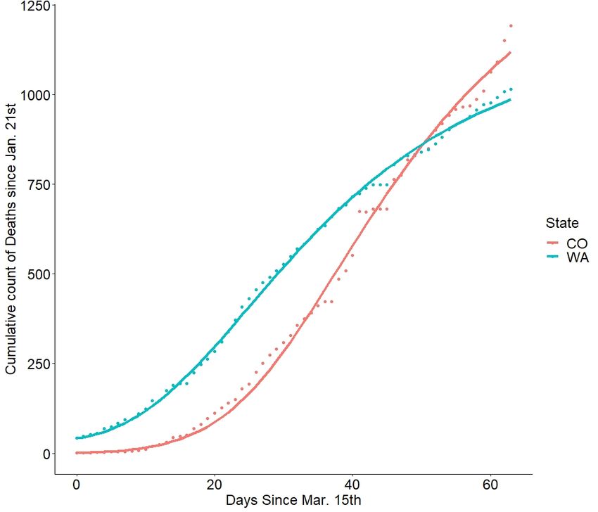
the primary goal of US public health measures has been to slow COVID-19 in-
fection rates enough that hospitals are not overwhelmed by a large influx of
diseased individuals, also phrased as “flattening the curve”. Until the recent
vaccine roll-out, this goal was mostly achieved through physical distancing –
any measure that increases the average distance or number of barriers between
individuals from different households. Physical distancing is often defined by
the closing of workplaces, schools, and non-essential businesses [34], but the
wearing of personal protective equipment (PPE) like gloves, face-coverings, and
eye protection also match this broad definition. Physical distancing measures
have been invaluable for mitigating COVID-19 spread, lowering the growth rate
of the disease [9] and preventing at least half a million COVID-19 cases [34].
However, physical distancing is not without drawbacks.
    Physical distancing imposes significant economic and psychological costs
that are themselves the common subject of COVID-19 models [29]. Closing
businesses and restricting travel in response to the COVID-19 pandemic dis-
rupted US supply chains [14], exacerbated social inequalities [11], and increased
rates of anxiety and depression [6]. There’s even evidence to suggest that physi-
cal or social distancing may increase the spread of conspiracy theories [13]. Fur-
thermore, physical distancing measures are ultimately voluntary and experts
expect such measures to be less effective as lockdowns continue and isolated
individuals inevitably grow bored [24]. News outlets report numerous stories
of Americans resisting physical distancing measures, especially the wearing of
masks [8]. Physical distancing could be the best tool America has for halting the
spread of future COVID-19 variants but considering supplementary strategies
may limit the need for physical distancing, and therefore its consequences, in
future pandemics.
    We present a model that considers two non-physical distancing strategies
to prevent overwhelming hospitals with COVID-19 infections: (1) hospitalizing
fewer patients with COVID-19 and (2) increasing hospital capacity for COVID-
19 patients. The former can be accomplished by selectively hospitalizing only
serious COVID-19 cases, allowing less serious cases to self-isolate, while the
latter can be accomplished by increasing the number of ICU beds, ventilators,
PPE, and hospital staff. For simplicity, we focus on just ICU bed counts as a
measure of hospital capacity and only consider the states of Washington (WA)
and Colorado (CO) because of their similar case numbers but different peak
infection times from March - May 2020.
    Washington was the first state in the U.S. to have confirmed COVID-19
infections [28]. When COVID-19 first arrived there, it spread rapidly among
the elderly and nurses at long-term care facilities [25]. Newspapers at the time
reported a reasonable fear that there would not be enough hospital beds in
the whole state to care for the coming wave of COVID-19 infected patients
[4]. WA enacted stay-at-home orders in mid-March and many other states like
CO soon followed, as uncontrolled community-level transmission was already
occurring in other states [23]. In fact, early in the pandemic, CO had one of
the highest death counts in the US, just behind California [30]. Thanks to
policies to expand hospital capacity and enact physical distancing, Washington

                                                                                     318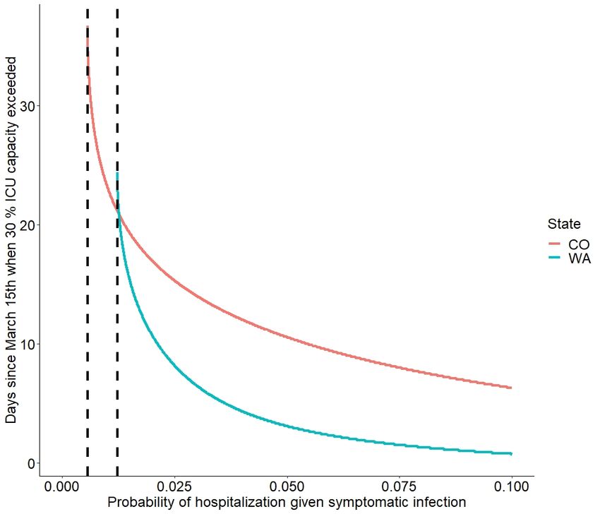
and CO avoided exceeding the state-wide limit on hospital beds from March
- May. Thus, knowing the relative benefits of increasing hospital capacity vs
decreasing hospitalization in either of these states is still relevant today. Neither
of these strategies should replace physical distancing, of course, but they can
still contribute to mitigation efforts.

3     Methods
We employed a system of ordinary differential equations to model the spread
of COVID-19 in WA and CO. We chose to model just WA and CO because of
their similar case numbers during their initial outbreaks, their high-quality re-
porting according to COVID-tracking project (see Table S1), but different peak
infection times. We further focused on data from only the period of March 15th
– May 18th as this captured the majority of the first “infection wave” in both
states. Focusing on this single period allowed us to avoid explicitly modeling
complicated changes in human behavior that eventually lead to multiple waves
of infection in both states. This focus also makes our study more relevant to
future initial pandemic scenarios where public health agencies have relatively
little data on disease dynamics. Most of the model parameters were estimated
from previous studies on COVID-19 spread. The remaining parameters were
estimated by minimizing the sum of squared errors between the model and data
on cumulative deaths over time. Our model was calibrated to mortality data
only because, due to testing limitations, counts of COVID-19 deaths are gener-
ally considered more reliable than counts of COVID-19 cases [3]. All simulations
and analyses were conducted in R [31]. Simulation, optimization, and data vi-
sualization were all executed with the deSolve, Flexible Modeling Environment
(FME), and ggplot2 packages respectively [35],[36],[41].

3.1    Gathering Data
All of the datasets input into our model are listed in Table S2, along with hyper-
links to their associated websites. Counts of COVID-19 deaths during the period
of March 15th – May 18th were downloaded from the novel coronavirus infection
map hosted by the University of Washington. Counts of COVID-19 hospital-
izations were downloaded from a publicly available database hosted by Definitive
Healthcare, a healthcare data analytics company (https://www.definitivehc.com/about).
To correct for under-reporting of hospitalizations, data on hospitalization re-
sponse rates were downloaded from each state’s respective Department of Health
(DOH) website. This data has since been removed from the WA DOH website,
but a copy of the dataset is included in the supplemental (Table S3). Next, the
number of ICU beds in WA was downloaded directly from the WA DOH web-
site, but this information could not be found on the CO DOH website. Thus,
a report of 2018 ICU bed counts from a local CO news organization was used
instead. Finally, population size estimates for both states were acquired from
their respective US Census Bureau websites.

                                                                                        319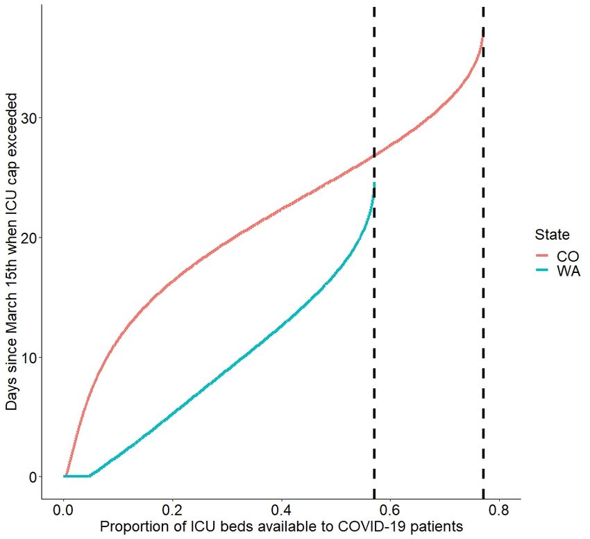
3.2 Correction for under-reporting by hospitals
Not all hospitals report counts of COVID-19 cases to their state governments
every day. For the states we studied, fewer hospitals reported COVID-19 hos-
pitalizations during weekends than weekdays (see Tables S3 and S4). The lack
of daily reporting partly contributes to hospitalization reports underestimating
the true number of hospitalizations. To account for under-reporting of hospi-
talizations, we applied a simple correction based on the assumption that the
ratio of hospitalizations to number of hospitals was the same for the sample of
reporting hospitals in a state as it is for all hospitals in a state. In other words:
U u
=
K k
Where U is the number of hospitalizations in the entire state, K is the number
of hospitals in the entire state, u is the number of reported hospitalizations, and
k is number of reporting hospitals. U is the only unknown in this equation,
meaning it can be calculated as:
Ku
U=
k
To apply this correction to the entire time series, we wrote U and u as
functions of time U(t) and u(t) respectively:
Ku(t)
U (t) =
k
The WA DOH only counted the number of reporting hospitals for May 9th
– May 15th, so data from this period was extrapolated to the entire time span
of March 15th – May 18th (see Table S3). There are 92 acute care hospitals in
the entire state, but only 66 hospitals reported case counts every day for May
9th – May 15th on average. Thus:
92u(t)
U (t) =
66
The CO DOH website also reports the percentage of hospitals that update
COVID-19 data. However, these data are deleted from the website weekly.
Thus, the average percentage of hospitals reporting data had to be estimated
from data from July 4th – July 9th (see Table S4). About 75.43 percent of CO
hospitals reported COVID-19 cases every day during this period on average.
Thus, the applied correction was:
100u(t)
U (t) =
75.43
3.3 Model formulation
Our system of ordinary differential equations included a total of 7 state variables
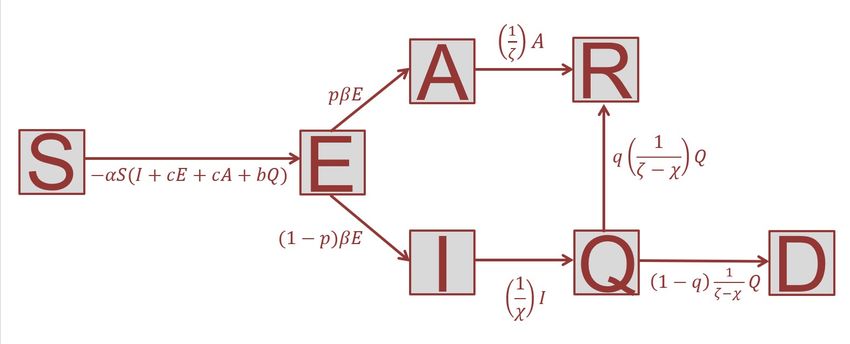
and 8 parameters, which are defined in Tables 1 and diagrammed in Figure 1.
320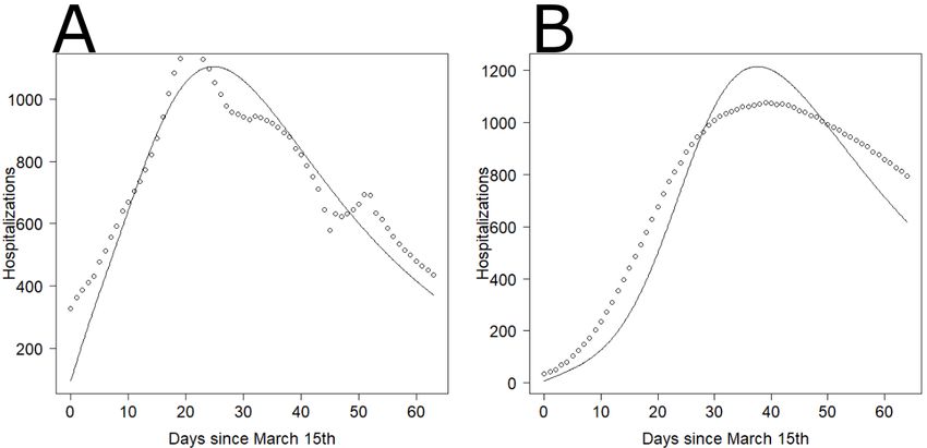
Figure 1: A compartment diagram depicting the system of ordinary differential
equations used in this study. See Tables S5 and S6 for variable and parameter
definitions.

From Figure 1, the full set of differential equations describing the spread of
COVID-19 in our model can be written as:
                       dS
                          = −αS (I + cE + cA + bQ)                         (1)
                       dt
                     dE
                        = αS (I + cE + cA + bQ) − βE                       (2)
                     dt

                           dA            1
                               = pβE −       A                             (3)
                           dt            ζ
                            dI               1
                               = (1 − p) βE − I                            (4)
                            dt               χ
                             dQ  1     1
                                = I−      Q                                (5)
                             dt  χ   ζ −χ
                            dR      1    1
                               =q      Q+ A                                (6)
                            dt    ζ −χ   ζ
                            dD             1
                               = (1 − q)      Q                            (7)
                            dt           ζ −χ
   We lastly define the number of hospitalized individuals at any moment in
time H(t) as:

                                 H(t) = hQ                                 (8)
    Where h ∈ [0, 1]. In other words, the number of hospitalized individuals
is assumed to be a constant proportion of the total number of quarantined
individuals, which includes both hospitalized and home-bound individuals.

                                                                                 321
Table 1: Definitions of parameters and state variables in SEAQIRD model.
Variable Definition Value Reference
Contact rate between sus-
α fitted NA
ceptible and infected
inverse of incubation pe-
β 1/3.60 days Li et al. 2020
riod
Verity et al.
ζ recovery time 24.7 days
2020
time until self-isolation
χ 1 day NA
once symptoms appear
Li et al.
probability of asymp-
2020;
p tomatic infection, given 0.86 or 0.425
Lavezzo
exposure
et al. 2020
probability of surviving a Wu et al.
q 0.986
symptomatic infection 2020
infectiveness of quaran-
tined individuals relative
b 0.1 NA
to non-quarantined in-
fected individuals
infectiveness of exposed
and asympotmatic indi-
c viduals relative to non- 0.55 Li et al. 2020
quarantined infected indi-
viduals
number of susceptible in-
S NA NA
dividuals
number of exposed, but
E NA NA
not infectious individuals
number of infected, but
A NA NA
asymptomatic individuals
number of infected, symp-
Q tomatic, and quarantined NA NA
individuals
number of infected,
I symptomatic, and non- NA NA
quarantined individuals
number of recovered indi-
R NA NA
viduals
number of dead individu-
D NA NA
als
Equations 1 through 7 will be referred to as the SEAQIRD model for the
322remainder of the paper. The SEAQIRD model begins with assuming that sus-
ceptible individuals are exposed to COVID-19 at rates proportional to how often
they contact individuals harboring SARS-CoV-2 (α).These individuals fall into
multiple categories: symptomatic infected (I), exposed but undetermined symp-
tom development (E), asymptomatic infected (A), and symptomatic isolated
infected (Q, for quarantined, which can mean either ”home-bound” or ”hospi-
talized”). The scaling factors c and b are meant to reflect the “infectiveness” of
individuals in the E, A, and Q compartments relative to the I compartment. We
chose c to be 0.55, reflecting the finding that asymptomatic individuals are 55
percent as infectious as symptomatic individuals [19]. We assumed b to be 0.1,
reflecting how isolated individuals ideally contact susceptible individuals only
rarely.
Once an individual is exposed (E) to SARS-CoV2, they were assumed to
have a probability p of becoming asymptomatically infected (A) and a proba-
bility of 1–p of becoming symptomatically infected (I). Furthermore, the rate
at which E individuals transformed into A or I individuals was assumed to be
proportional the inverse of the incubation period, β, estimated as 1/6.6 days
[19]. Asymptomatic individuals were assumed to never perish from COVID-19
and to recover from the disease at a rate proportional to 1/ζ, the inverse of the
recovery period. The recovery period, ζ, was estimated from a previous study
on COVID-19 severity as 24.7 days [39]. This result agrees with other studies
on COVID-19 suggesting that infected asymptomatic individuals typically shed
SARS-CoV-2 viruses 15 – 26 days after initial infection [21].
Once an exposed individual (E) individual develops into a symptomatically
infected individual (I), they mix with the population for χ days before isolating
themselves (see equations 5 and 4). χ was assumed to be 1 day in all SEAQIRD
models. Once isolated, the infectiveness of symptomatic individuals was as-
sumed to drop to 0.1α. This rate was intentionally made non-zero to account
for any minor contact isolated individuals have with susceptible individuals,
since quarantine measures are rarely perfect. Once isolated (Q), individuals
had a probability q of recovering from the disease and a probability 1–q of dy-
ing (see equations 6 and 7). The value of q was estimated as 0.986, again based
on COVID-19 studies in China [42]. In addition, some of the rate constants in
equations 6 and 7 were assumed to be the inverse of recovery period – χ, where
the “-χ” accounts for the time symptomatic individuals spend mixing with the
population before isolating themselves.
For the sake of simplicity, we assume that recovered individuals (R) are not
susceptible to re-infection with SARS-CoV-2. This is not known to be strictly
true for SARS-CoV-2 infection in humans, but it is reasonable given how non-
human primates respond to SARS-CoV-2 infection [7].
3.4 Choosing initial conditions
Given that SARS-CoV-2 is a completely novel virus and there was no vaccine
available in March 2020, the entire populations of WA and CO were assumed
to be susceptible to SARS-CoV-2 infection. Thus, the number of susceptible
323individuals in either state on March 15th, S0 , was initially estimated as:
N = S0 + E0 + A0 + Q0 + I0 + R0 + D0
N − E0 − A0 − Q0 − I0 − R0 − D0 = S0 (9)
Here, N is the total population size of the state and the other variables are
the initial values for the given state’s SEAQIRD compartments. Importantly,
equation 9 only defined the initial estimate of S0 , but S0 was allowed to vary
during the model fitting process (see section 3.6).
Since COVID-19 mortality data is generally reliable, the number cumulative
deaths up until March 15th, D0 , was not adjusted in the raw data. On the other
hand, estimating the number of symptomatic, infected individuals required some
adjustment. Ideally, the initial number of I individuals (I0 ) could be calculated
as:
I0 = C0 − D0 − R0
Where C0 , D0 , and R0 are cumulative numbers of active COVID-19 cases,
deaths, and recoveries up until March 15th, respectively. For simplicity, R0 and
H0 were assumed to be small relative to C0 and D0 early in the pandemic,
leaving just:
I0 = C0 − D0
However, C0 is drastically underestimated for the US population. One pre-
print study suggests that increasing the number of cases in the US by 179 percent
would bring the US death rate down to a similar rate as South Korea, a country
with reliable infection counts, after accounting for demographic differences [17].
Thus, I0 was estimated as:
I0 = 2.79C 0 − D0
This calculation assumes that the correction for the US applies to individual
states as well. The initial number of exposed individuals (E0 ) and asymptomatic
infected individuals (A0 ) was assumed to be directly proportional to I0 . In the
absence of reliable data on these numbers, we decided:
E0 = 30I0
A0 = 8I0
because these numbers generated biologically reasonable model curves and
they reflect how the majority of COVID-19 transmission occurs through asymp-
tomatic individuals [19].
Finally, the initial number of symptomatic, isolated individuals (Q0 ) was
assumed to be:
324Q0 = 10H(0)
Here, H(0) is the number of individuals hospitalized with COVID-19 on
March 15th. In other words, for every individual hospitalized with COVID-
19, there were assumed to be nine other symptomatic individuals that were
self-isolating at home.
3.5 Sensitivity analysis
Once we developed the baseline SEAQIRD models (E0 = 30*I0 , Q0 = 10*H(0),
p = 0.86, q = 0.986, and χ = 1) for CO and WA conditions and parameter values
were chosen, we tested the sensitivity of the WA and CO SEAQIRD models in
two ways. First, we used the sensFun() command in the FME package to analyze
the local sensitivity of the SEAQIRD model to all of its initial conditions and
parameters [35]. This analysis was repeated twice, once for WA initial conditions
(see Figures S2A, S2B, and S3) and once for CO initial conditions (see Figures
S6A, S6B, and S7). Second, we then focused on the parameters p and q for
both SEAQIRD models since they had by far the most influence on the model
output. We re-ran both the WA and CO models under different values of p
and q values while holding all other initial conditions at their baseline values.
Estimates of p vary widely in published literature, so we ran the SEAQIRD
model with two different values of p (0.86 and 0.425) while holding all other
parameters and conditions at their baseline values (see Figures S9 - S12). The
first value of p comes from a study that estimated the fraction of cases that
went undocumented during a period of COVID-19 spread in China [19]. Cases
often go undocumented when infected individuals have symptoms that are too
mild for them to be concerned with getting tested for infection. Thus, we
reasoned this fraction should be close to the value of p. The second value of p
comes from a census in Italy where the authors directly observed 42.5 percent of
their COVID-19 infected participants lacking symptoms [18]. We also ran the
SEQIRD model with two different values of q, its baseline value of 0.986 and a
value of 0.972 (see Figures S13 - S16), which doubles the probability of dying
from a symptomatic infection relative to the baseline SEAQIRD model.
3.6 Fitting SEAQIRD to data
We used the Levenberg–Marquardt algorithm implemented in the FME package
to optimize α and S0 such that the sum of squared error between the SEAQIRD
model output and the curve of cumulative deaths over time for either WA or
CO was minimized. We only fit these two parameters because these are the
parameters that have the most influence on the model’s results besides p and q
(see Figures S2 and S7). However, unlike p and q these numbers could not be
reasonably estimated from previous studies. Furthermore, we could not fit ad-
ditional parameters with the paucity of data points we had without overfitting.
Finally, we also only chose to fit the SEAQIRD model to mortality data because
325estimates of other state variables, such as symptomatic infections, are probably
massively under-counted. In all model fitting cases, the initial estimate of S0
was given by equation 9 and the initial estimate of α was 3E-7, but these values
were allowed to vary within bounds during the fitting process. α was always
bounded between 3E-6 and 3E-8 while S0 was bounded between 0.05 and 1.5
times its initial estimate. These bounds were chosen because they produced
biologically reasonable results (see Figures 2, S1A, and S5A).
3.7 Estimating probability of hospitalization given symp-
tomatic infection
The number of individuals hospitalized with COVID-19 was assumed to be a
constant fraction of the number of individuals in compartment Q (see equation
8). After simulating the SEAQIRD model based on the initial conditions de-
scribed above, this fraction was estimated for each state model by plotting the
number of hospitalizations in the state against the number of quarantined indi-
viduals output by the fitted SEAQIRD model at each time point. The slope of
the ordinary least squares regression line through these points (see Figures S1B
and S5B) estimated the probability of hospitalization given symptomatic infec-
tion (h), since all quarantined individuals are either hospitalized or not.This
resulted in an obvious underestimation of h (see Figures S1C and S5C). Thus,
we also tried estimating h numerically by multiplying the H(t) function by 10000
different constants increasing from 0 to 0.1 in increments of 1E-5 and calculating
the sum of squared error between the resulting curve and hospitalization counts
over time. The constant that gave the lowest sum of squared error between
H(t) ∗ h and the curve of hospitalization counts over time, after correcting for
under-reporting, thus estimated h (see Figures 5A and 5B).
3.8 Estimating effect of decreased hospitalization and in-
creased bed cap on delaying bed shortage
Pre-pandemic surveys suggest that about 50 – 80 percent of ICU beds in America
are typically occupied at any given time [43]. Thus, we assumed that 30 percent
of ICU beds in either WA or CO could be reasonably allocated to COVID-19
infected patients during the modeling period, which is referred to as the hospital
“bed cap” at some points in the paper. Once the probability of hospitalization
given symptomatic infection (hereto referred to as the “hospitalization proba-
bility”) was estimated from the fit of SEAQIRD model to the hospitalization
data, we tested the effect of altering the probability of hospitalization and the
bed cap simultaneously by plugging 10000 different combinations of these two
numbers spanning values from 0 – 1, in increments of 1E-5, into the SEAQIRD
model (see Figures S4, S8, S10, S12, S14, S16).
3264 Results
4.1 Effective population sizes for COVID-19 transmission
Figure 2 presents the optimized baseline SEAQIRD model’s fits to mortality
data for CO and WA. The best fit parameters for α and S0 in under these condi-
tions were 5.990521e-07 and 4.814597e+05, respectively, for the WA SEAQIRD
model and 4.687143e-07 and 7.675917e+05, respectively, for the CO SEAQIRD
model (see Figure 2). The curves for the other state variables in the SEAQIRD
model, suggest that WA and CO had 39,805 and 53,742 symptomatic infected
individuals (I + Q), respectively, at their peak infection periods between March
15th and May 18th (see Figures S1 and S5). The number of asymptomatic
infected cases (E + A), on the other hand, peaked at 280,280 and 388,234
individuals for WA and CO respectively during this period. In the SEAQIRD
model, the peak number of hospitalizations occurred 24 and 37 days after March
15th for WA an CO, respectively. The actual peak in hospitalizations for these
states during the modeling period, however, occurred 21 days and 39 days after
March 15th, respectively. The probability of hospitalization given symptomatic
infection was estimated as 0.0290 (see Figure 3A) and 0.0236 (see Figure 3B)
for WA and CO, respectively. During the modeling period, CO started out as
having fewer death cases than WA, but then overtook WA death counts by the
end of the modeling period.
4.2 Effect of decreasing hospitalization on delaying bed
shortage
Hospitalizing fewer COVID-19 patients delayed the time at which the bed ca-
pacity for COVID-19 patients was exceeded (Figure 4). This effect increased as
fewer COVID-19 patients were hospitalized, according to the concave up shape
of the graph in Figure 4. The curves for both WA and CO reach asymptotes; in
other words, values of the hospitalization probability below which the bed cap
will never be exceeded. This occurred around a probability of 0.0123 for WA
and about 0.00567 for CO.
4.3 Effect of increasing bed cap on delaying bed shortage
The graph of how the number of days until the bed cap is exceeded based on
the proportion of available ICU beds looks markedly different between WA and
CO (Figure 5). The curve for CO initially shows a concave down shape, but
inflects around a value of of 0.5. The curve for WA, on the other hand, has
a mostly concave up shape. Both curves approach an asymptote (see dotted
lines in Figure 5) as the bed cap increases. For WA, this asymptote occurred
around a bed cap of 57.5 percent of the maximum. The asymptote for CO, on
the other hand, occurred at a bed cap of about 77.6 percent of the maximum.
For a non-zero proportion of bed availability, bed caps were always exceeded
later in CO than in WA.
327Figure 2: Points are raw counts of deaths due to COVID-19 since Jan. 21st
- colored by the state in which the deaths occurred - and the lines are the
SEAQIRD model fits to these points. For both models E0 = 30*I0 , Q0 =
10*H(0), p = 0.86, q = 0.986, and χ = 1.
4.4 SEAQIRD sensitivity to conditions and parameters
Once the SEAQIRD model was fit to each state’s data, we tested the local
sensitivity of the SEAQIRD model to its initial conditions and α. We first
used the local sensitivity analysis functions implemented in the FME package
to identify the initial conditions with the largest influence on model output. S0 ,
α, and D0 , are well-estimated either directly from data or from the model fitting,
whereas the values of the remaining conditions were assumed. Thus, we took
the two parameters the SEAQIRD model was most sensitive to, p and q, altered
their values, and recorded the effect on the SEAQIRD model’s predictions. We
ran the SEAQIRD model with p set to 0.86 and 0.425, while keeping all other
parameters and initial conditions at their baseline values. We also tried setting
q to either 0.986 (it’s value in the baseline model) or 0.972 (which doubles the
probability of dying from infection). The different values for p gave very different
curves for both the WA and CO SEAQIRD models (see Figures S9 and S11),
as did the different values of q (see Figures S13 and S15). However, even in
these alternative scenarios, the effects of altering the hospitalization probability
retained a more concave upward shape than altering the bed cap (see Figures
328Figure 3: (A)Points are counts of hospitalized COVID-19 patients in all WA hos-
pitals by day, corrected for underreporting by hospitals. Curve is Q(t) function
output from SEAQIRD model multiplied by the probability of hospitalization
given symptomatic infection, which was numerically estimated as 0.0289829.
(B) Points are counts of hospitalized COVID-19 patients in all CO hospitals by
day, corrected for underreporting by hospitals. Curve is Q(t) function output
from SEAQIRD model multiplied by the probability of hospitalization given
symptomatic infection, which was estimated to be about 0.02357236. For both
(A) and (B), SEAQIRD initial conditions included E0 = 30*I0 , Q0 = 10*H(0),
p0 = 0.86, q = 0.986 and χ = 1.
S10, S12, S14, S16).
5 Discussion
Some of SARS-CoV-2’s defining characteristics are that a large fraction of in-
fected individuals do not develop symptoms and that there’s a significant pre-
symptomatic period during which an individual can still spread the virus. This
has led to massive levels of undocumented infection; some pre-print articles es-
timate that 19 million Americans have caught COVID-19, only a small fraction
of which are laboratory confirmed cases [22]. We developed a novel system of
differential equations to account for these asymptomatic and presymptomatic
phases of COVID-19 infection, which happened to be similar to other models
used to model COVID-19 spread [22]. This system was fit to data on COVID-
19 mortality, the most reliable data available on COVID-19 spread, in two US
states. These different states had different infection dynamics and different peak
infection dates. Including infection peaks in the analysis was especially impor-
tant because deterministic models like SEAQIRD can be especially misleading
329Figure 4: Dotted vertical lines represent asymptotes – the probability beyond
which the ICU bed cap would not be exceeded from March 15th – May 18th.
Both models used their baseline values for initial conditions and parameters.
when fit with only pre-peak data [10]. We then compared the effects of decreas-
ing the probability of hospitalization given symptomatic infection and increasing
the proportion of ICU beds available to COVID-19 patients on delaying when
the number of hospitalized COVID-19 patients exceeded the allotted ICU bed
capacity. Under the conditions simulated here, we observed that when the prob-
ability of hospitalization is already low, decreasing it further can have a large
effect on delaying an ICU bed shortage. Meanwhile, altering the proportion of
ICU beds available to COVID-19 patients had different effects on when a bed
shortage was reached in the two states. This finding was very robust for both
the WA and CO models under multiple sets of initial conditions and parameter
values.
5.1 Altering bed cap has different effects on delaying a
bed shortage in WA and CO
Our analyses focused on two parameters of the SEAQIRD model that best
represented potential interventions for preventing a hospital bed shortage: the
number of beds available to COVID-19 patients (expressed as a proportion of all
330Figure 5: Dotted vertical lines represent asymptotes – proportion of ICU bed
availability beyond which the ICU bed cap would not be exceeded from March
15th – May 18th . For both models E0 = 30*I0 , Q0 = 10*H(0), p = 0.86, q =
0.986, χ = 1.
beds in the state) and the probability of a symptomatic, infected individual of
being hospitalized (h). We altered both of these parameters and observed their
effects on when an ICU bed shortage (defined as the number of hospitalized
individuals exceeding the number of available beds) was reached in WA and
CO.
First, we altered one parameter while holding the other constant. For both
WA and CO, decreasing the hospitalization probability had larger effects on
delaying a bed shortage if this probability was already small (see Figure 4).
However, the effect of increasing the bed cap differed drastically between the
WA and CO models. Increasing the bed cap has a more sigmoid relationship
with delaying a bed shortage in CO than it does in WA (see Figure 5). This is
potentially due to differences in the total number of cases relative to hospital
beds in both states. The maximum number of infected individuals (I + A)
was much higher in CO than in WA (53,742 vs 39,805) while the number of
ICU beds was also much lower in CO than WA (973 vs 1564). These factors
combined could have made increasing the number of ICU beds in CO initially
less effective at halting a bed shortage, leading to the sigmoid relationship in
331Figure 5. We also altered both the hospitalization probability and bed cap at
the same time and observed similar results (see Figures S10, S12, S14, S16).
Overall, our findings do not conflict with current CDC guidelines that tell sick
individuals to not go to hospitals unless they are experiencing severe COVID-19
symptoms [40].
5.2 SEAQIRD predictions are robust to initial conditions
and parameter values
The parameters with by far the largest influence on SEAQIRD dynamics are
the probability of developing a symptomatic infection given COVID-19 exposure
(p) and the probability of dying from a symptomatic COVID-19 infection (q).
Early studies on COVID-19 suggested that p could be fairly low – around 20
percent or less [16], [26]. Later studies suggested that this probability is likely
higher - upwards of 50 percent [18],[19]. Changing the values of p and q in
the SEAQIRD model had a large influence on the model output relative to the
other parameters and initial conditions (see Figures S2A, S3, S6A, S7). Thus,
we suspect that changes in p and q over time or between different groups of
people are mainly responsible for the poor fits between the SEAQIRD model
and hospitalization data (see Figure 3A and 3B). Rewriting these parameters to
be dependent on demographic characteristics, such as age, could improve these
fits.
5.3 Low effective population size for COVID-19 transmis-
sion in CO and WA
The effective population size of both the WA and CO SEAQIRD models was
orders of magnitude lower than the actual population sizes of these states as
estimated by the US census. This discrepancy is partly due to the lack of any
lockdown effects in the SEAQIRD model. Thus, COVID-19 was restricted to
spreading among only a subset of the WA and CO populations. The lack of lock-
down effects is arguably SEAQIRD model’s most obviously violated assumption.
WA lockdowns began on March 23rd 2020 [15], not long into the simulation,
closely followed by CO on March 26th [23]. However, there is some pre-print
work suggesting that US individuals were already relaxing physical distancing
measures by mid-April, perhaps limiting the lockdown effect in our data [44].
Other phenomenon could have also contributed to the small effective population
size in the SEAQIRD model. For example, there are well-documented cases of
individuals unexposed to COVID-19 having antibodies that react to SARS-CoV-
2 particles [32]. There’s also population-level evidence suggesting that certain
pre-existing vaccines may have trained immune systems against COVID-19, al-
though these vaccines are not common in the US [5],[12]. Nonetheless, it is
possible that pre-existing and trained immunity may have removed individuals
from the susceptible populations in CO and WA, explaining why COVID-19
only spread among a small subset of these populations in the SEAQIRD model.
Incorporating lockdown effects, pre-existing immunity, and trained immunity
332into SEAQIRD-like models may improve their predictions. Understanding how
these nuances affect hospitalizations will be incredibly important as the US
continues to control the spread of COVID-19 and any variants that arise.
References
[1] E. Abdollahi, M. Haworth-Brockman, and Y. Keynan, et al., Simulating
the effect of school closure during COVID-19 outbreaks in Ontario, Canada.
BMC Med., 18 (2020), pp. 2-8.
[2] N. Aguirre-Duarte, Can people with asymptomatic or pre-symptomatic
COVID-19 infect others: a systematic review of primary data. medRxiv,
2020.04.08.20054023, 2020.
[3] C. Anastassopoulou, L. Russo, and A. Tsakris, et al., Data-based anal-
ysis, modelling and forecasting of the COVID-19 outbreak. PLoS ONE, 15,
e0230405.
[4] M. Bellisle and R. La Corte, Washington scrambles for hospital beds,
https://www.columbian.com/news/2020/mar/19/washington-scrambles-for-
hospital-beds/ (19 March 2020)
[5] B. Brook, D. J. Harbeson, and C. P. Shannon, et al., BCG vaccina-
tion–induced emergency granulopoiesis provides rapid protection from neona-
tal sepsis, Sci. Transl. Med., 12. (2020), eaax4517.
[6] S. K. Brooks, R. K. Webster, and L. E. Smith, et al., The psychological
impact of quarantine and how to reduce it: rapid review of the evidence. The
Lancet, 395 (2020), pp. 912–920.
[7] A. Chandrashekar, J. Liu, and A. J. Martinot, et al., SARS-CoV-2 infection
protects against rechallenge in rhesus macaques Science, 369 (2020), pp. 812-
817.
[8] S.Andrew, The psychology behind why some people won’t wear masks
https://www.cnn.com/2020/05/06/health/why-people-dont-wear-masks-
wellness-trnd/index.html. (6 May 2020).
[9] C. Courtemanche, J. Garuccio, and A. Le, et al., Strong Social Distancing
Measures In The United States Reduced The COVID-19 Growth Rate. H. Aff.
Mill., 39 (2020), pp. 1237–1246.
[10] J. Daunizeau, R. J. Moran, and J. Mattout, et al., On the reliability
of model-based predictions in the context of the current COVID epidemic
event: impact of outbreak peak phase and data paucity, preprint, medRxiv,
2020.04.24.20078485, 2020.
[11] A. van Dorn, R. E. Cooney, and M. L. Sabin, COVID-19 exacerbating
inequalities in the US Lancet Lond. Engl., 395 (2020), pp. 1243–1244.
333[12] L. E. Escobar, A. Molina-Cruz, and C. Barillas-Mury, BCG vaccine pro-
tection from severe coronavirus disease 2019 (COVID-19), Proc. Natl. Acad.
Sci. U. S. A., 117 (2020), pp17720–17726.
[13] D. Graeupner and A. Coman, The dark side of meaning-making: How social
exclusion leads to superstitious thinking. J. Exp. Soc. Psychol., 69 (2017), pp.
218–222.
[14] D. Guan, D. Wang, and S. Hallegatte, et al., Global supply-chain effects of
COVID-19 control measures, Nat. Hum. Behav., 4 (2020), pp. 577–587.
[15] J. Inslee, Inslee announces “Stay Home, Stay Healthy” order,
https://www.governor.wa.gov/news-media/inslee-announces-stay-home-
stay-healthy
[16] J. R. Koo, A. R. Cook, and M. Park, et al., Interventions to mitigate early
spread of SARS-CoV-2 in Singapore: a modelling study, Lancet Infect. Dis.,
20 (2020), pp. 678–688.
[17] A. Lachmann, Correcting under-reported COVID-19 case numbers,
preprint, medRxiv 2020.03.14.20036178, 2020.
[18] E. Lavezzo, E. Franchin, and C. Ciavarella, et al., Suppression of a SARS-
CoV-2 outbreak in the Italian municipality of Vo’ Nature, 584 (2020), pp.
425-429.
[19] R. Li, S. Pei, and B. Chen, et al., Substantial undocumented infection facil-
itates the rapid dissemination of novel coronavirus (SARS-CoV-2), Science,
368 (2020), pp. 489–493.
[20] K. Liu, Y. Chen, and R. Lin, et al., Clinical features of COVID-19 in elderly
patients: A comparison with young and middle-aged patients, J. Infect., 80
(2020), pp. e14–e18.
[21] Q.-X. Long, X.-J. Tang, and Q.-L. Shi, et al., Clinical and immunological
assessment of asymptomatic SARS-CoV-2 infections, Nat. Med., 26 (2020),
pp. 1200-1204.
[22] A. Mahajan, R. Solanki, and N. Sivadas, Estimation of Undetected Symp-
tomatic and Asymptomatic cases of COVID-19 Infection and prediction of its
spread in USA, medRxiv 2020.06.21.20136580, 2020.
[23] K. Marshall, G. M. Vahey, and E. McDonald, et al., Exposures Before
Issuance of Stay-at-Home Orders Among Persons with Laboratory-Confirmed
COVID-19 — Colorado, March 2020. Morb. Mortal. Wkly. Rep., 69, pp.
847–849.
[24] C. S. Martarelli, and W. Wolff, Too bored to bother? Boredom as a po-
tential threat to the efficacy of pandemic containment measures, preprint,
PsyArXiv/s41599-020-0512-6, 2020.
334[25] T. M. McMichael, D. W. Currie, and S. Clark, et al., Epidemiology of Covid-
19 in a Long-Term Care Facility in King County, Washington, N. Engl. J.
Med., 382 (2020), pp. 2005–2011.
[26] K. Mizumoto, K. Kagaya, and A. Zarebski, et al., Estimating the asymp-
tomatic proportion of coronavirus disease 2019 (COVID-19) cases on board
the Diamond Princess cruise ship, Yokohama, Japan, 2020, Euro Surveill.,
25 (2020), 22.
[27] S. M. Moghadas, A. Shoukat, and M. C. Fitzpatrick, et al., Projecting
hospital utilization during the COVID-19 outbreaks in the United States, Proc.
Natl. Acad. Sci., 117 (2020), pp. 9122-9126
[28] M. Mossa-Basha, J. Medverd, and K. Linnau, et al., Policies and Guidelines
for COVID-19 Preparedness: Experiences from the University of Washington.
Radiology, (2020), 201326.
[29] S. C. Newbold, D. Finnoff, and L. Thunström, et al., Effects of Physical
Distancing to Control COVID-19 on Public Health, the Economy, and the
Environment, Environ. Resour. Econ., (2020), pp. 1-25.
[30] I. J. Ramı́rez and J. Lee, COVID-19 Emergence and Social and Health
Determinants in Colorado: A Rapid Spatial Analysis Int. J. Environ. Res.
Public. Health, 17 (2020), 3856.
[31] R Core Team, R: A language and environment for statistical computing. R
Foundation for Statistical Computing, https://www.R-project.org/ (2020).
[32] A. Sette and S. Crotty, Pre-existing immunity to SARS-CoV-2: the knowns
and unknowns, Nat. Rev. Immunol., 20 (2020), pp. 457–458.
[33] A. Shoukat, C. R. Wells, and J. M. Langley, et al., Projecting demand for
critical care beds during COVID-19 outbreaks in Canada, CMAJ, 192 (2020),
pp. e489–e496.
[34] M. J. Siedner, G. Harling, and Z. Reynolds, et al., Social distancing to slow
the US COVID-19 epidemic: Longitudinal pretest–posttest comparison group
study, PLoS Med., 17 (2020), e1003244.
[35] K. Soetaert and T. Petzoldt, Inverse Modelling, Sensitivity and Monte
Carlo Analysis in R Using Package FME, J. Stat. Softw., 33 (2010), pp.
1–28.
[36] K. Soetaert, T. Petzoldt, and R. W. Setzer, Solving Differential Equations
in R: Package deSolve, J. Stat. Softw., 33 (2010), pp. 1–25.
[37] D.B.G. Tai, A. Shah, and C. A. Doubeni, et al. The Disproportionate Im-
pact of COVID-19 on Racial and Ethnic Minorities in the United States, Clin.
Infect. Dis., (2020), pp. 1-4
335[38] S. Y. Tartof, L. Qian, and V. Hong, et al., Obesity and Mortality Among
Patients Diagnosed With COVID-19: Results From an Integrated Health Care
Organization, Ann. Intern. Med., (2020), pp. 1-10.
[39] R. Verity, L. C. Okell, and I. Dorigatti, et al., Estimates of the severity
of coronavirus disease 2019: a model-based analysis, Lancet Infect. Dis., 20
(2020), pp. 669-677.
[40] Center for Disease Control and Prevention (CDC) What to Do If You
Are Sick, https://www.cdc.gov/coronavirus/2019-ncov/if-you-are-sick/steps-
when-sick.html (15 August 2020).
[41] H. Wickham, ggplot2: Elegant Graphics for Data Analysis, Springer-Verlag
Inc., New York, NY, 2016.
[42] J. T. Wu, K. Leung, and M. Bushman, et al., Estimating clinical severity
of COVID-19 from the transmission dynamics in Wuhan, China, Nat. Med.,
26 (2020), pp. 506–510.
[43] H. Wunsch, J. Wagner, and M. Herlim, ICU Occupancy and mechanical
ventilator use in the United States, Crit. Care Med., 41 (2013), pp. 2712-
2719.
[44] J. Zhao, M. Lee, and S. Ghader, et al., Quarantine Fatigue: first-ever
decrease in social distancing measures after the COVID-19 outbreak before
reopening United States, preprint, arXiv:2006.03716 [cs], 2020.
336You can also read