Dynamics of seasonally frozen ground in the Yarlung Zangbo River Basin on the Qinghai-Tibet Plateau: historical trend and future projection
←
→
Page content transcription
If your browser does not render page correctly, please read the page content below
Environmental Research Letters

LETTER • OPEN ACCESS

Dynamics of seasonally frozen ground in the Yarlung Zangbo River
Basin on the Qinghai-Tibet Plateau: historical trend and future projection
To cite this article: Fang Ji et al 2020 Environ. Res. Lett. 15 104081

View the article online for updates and enhancements.

                                This content was downloaded from IP address 46.4.80.155 on 16/10/2020 at 19:15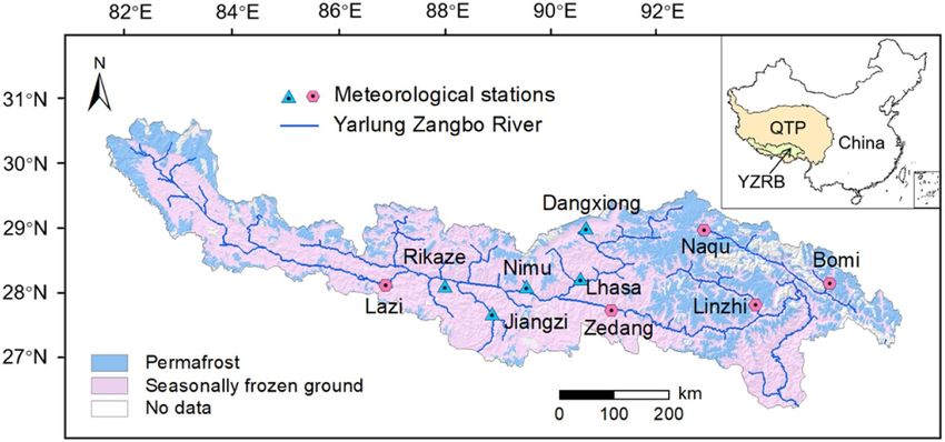
Environ. Res. Lett. 15 (2020) 104081 https://doi.org/10.1088/1748-9326/abb731
Environmental Research Letters
LETTER
Dynamics of seasonally frozen ground in the Yarlung Zangbo River
OPEN ACCESS
Basin on the Qinghai-Tibet Plateau: historical trend and future
RECEIVED
7 February 2020 projection
REVISED
21 August 2020 Fang Ji1,2,3, Linfeng Fan2,3, Charles B Andrews2,3,4, Yingying Yao5 and Chunmiao Zheng2,3
ACCEPTED FOR PUBLICATION 1
10 September 2020 School of Environment, Harbin Institute of Technology, Harbin, People’s Republic of China
2
Guangdong Provincial Key Laboratory of Soil and Groundwater Pollution Control, School of Environmental Science and Engineering,
PUBLISHED
Southern University of Science and Technology, Shenzhen, People’s Republic of China
7 October 2020 3
State Environmental Protection Key Laboratory of Integrated Surface Water-Groundwater Pollution Control, School of Environmental
Science and Engineering, Southern University of Science and Technology, Shenzhen, People’s Republic of China
Original content from 4
S. S. Papadopulos and Associates, Inc., Bethesda, MD, United States of America
this work may be used 5
under the terms of the
Department of Earth and Environmental Science, School of Human Settlements and Civil Engineering, Xi’an Jiaotong University, Xi’an,
Creative Commons People’s Republic of China
Attribution 4.0 licence.
E-mail: zhengcm@sustech.edu.cn and fanlf@sustech.edu.cn
Any further distribution
of this work must Keywords: seasonally frozen ground, ground temperature, climate change, Yarlung Zangbo River Basin, Qinghai-Tibet Plateau
maintain attribution to
the author(s) and the title Supplementary material for this article is available online
of the work, journal
citation and DOI.
Abstract
Seasonally frozen ground (SFG) is a critical component of the Earth’s surface that affects energy
exchange and the water cycle in cold regions. The estimation of SFG depth has generally required
intensive parameterization which has limited estimates in data-scarce regions such as the
Qinghai-Tibet Plateau (QTP). We propose a simple yet robust modeling framework employing
ground surface temperatures as major model inputs to assess the spatiotemporal patterns of the
SFG depth in the Yarlung Zangbo River Basin (YZRB) on the QTP. The model was calibrated using
SFG depth measurements throughout the YZRB from 1980 to 2010. Results suggest that the SFG
depth in the YZRB has decreased at a rate of 2.50 cm · a−1 from 1980 to 2010. Future projections
indicate that the SFG depth in the YZRB will continue to decrease in response to future warming.
The present SFG may no longer exist by 2180 under the RCP 8.5 scenario (if not considering the
transition of permafrost to SFG). The proposed modeling framework provides an important basis
for the evaluation of the hydrological cycles (e.g. surface water-groundwater interactions) in cold
regions under changing climatic conditions.
1. Introduction The Qinghai-Tibet Plateau (QTP) is the source
region of several important large rivers (e.g. the
Seasonally frozen ground (SFG) is defined as the por- Yellow River, Yangtze River, Lancang River, and
tion of soil that freezes in winter and thaws in summer Yarlung Zangbo River) and is often referred to as the
in cold regions (Evans and Ge 2017). The presence of water tower of the southeast Asia (Jin et al 2009).
SFG affects the seasonal infiltration in the vadose zone The Yarlung Zangbo River Basin (YZRB) is one of
and thus the groundwater recharge (Ge et al 2011). the most densely populated regions on the QTP and
SFG is a thermal condition dependent on ground seasonally frozen soil broadly occurs here (Zhong
thermal regime. With soil freezing and thawing, SFG et al 2014). Many studies have reported that the dra-
influences the thermal and hydraulic conditions of matic climate warming in recent decades has substan-
the soil layer and thus impacts the regional hydrolo- tially accelerated the decrease of the SFG depth in
gical cycle and ecosystem function (Yang et al 2002, this region (Zhao et al 2004, Pang et al 2011). How-
Hansson et al 2004, Guo and Wang 2016). Assess- ever, long-term observations of SFG depth are lack-
ing the spatiotemporal pattern of the SFG depth is ing due to the high cost of direct measurements and
essential for water resources management and envir- maintenance of monitoring systems in cold regions.
onmental conservation in cold regions. Hence, the assessment of the SFG depth over the
© 2020 The Author(s). Published by IOP Publishing Ltd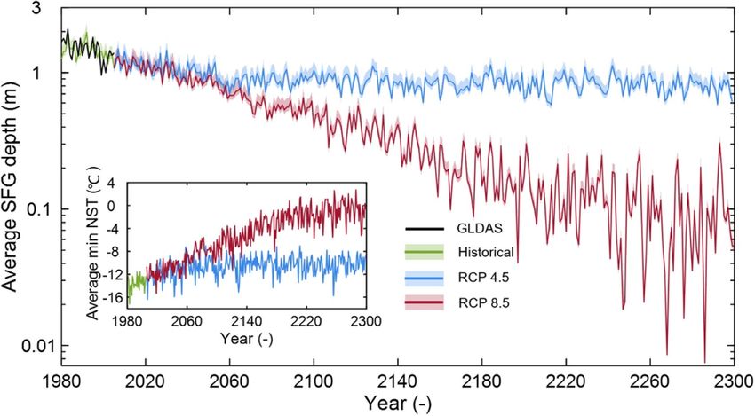
Environ. Res. Lett. 15 (2020) 104081 F Ji et al
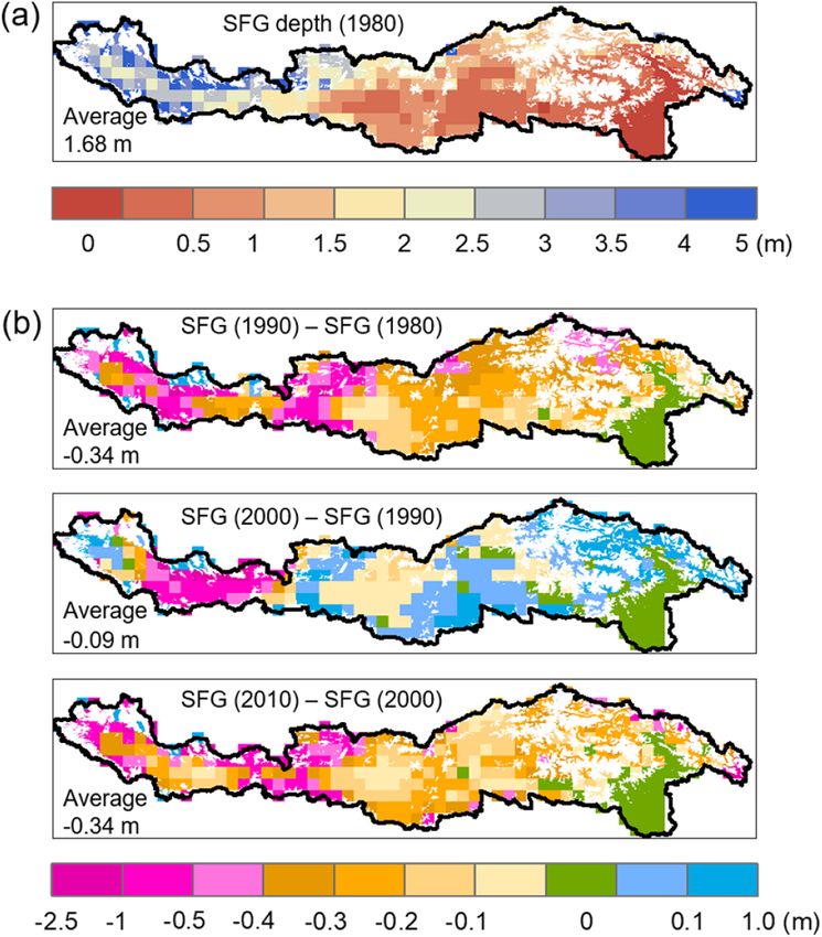
Figure 1. Geographical location, spatial distribution of SFG, permafrost (Zou et al 2017), and meteorological stations in the
YZRB on the QTP. All meteorological stations are used for calibration of GLDAS data, and the stations indicated with blue
triangles were used for the calibration of the ‘GT-SFG depth’ model. The inset map in the upper-right corner shows the
geographical locations of the YZRB (yellow area) and the QTP (orange area) within China.
large spatial scales often rely on computational mod- limits their application in data-scarce regions such as
els. Numerical schemes (e.g. finite element and finite the QTP.
diffrenence methods) that solve heat transport equa- Hence, the aim of this study is to develop a simple
tions are often incorporated in hydrological models yet robust approach to estimate the long-term spa-
to simulate the soil freeze-thaw process (Gouttevin tially resolved patterns of the SFG depth in cold
et al 2012, Rawlins et al 2013, Zhang et al 2017). regions. We utilize a semi-empirical ground tem-
For instance, the SUTRA model (Voss and Provost perature (GT) model using ground surface (0–5 cm
2010) couples heat transport with groundwater flow below the surface cover) temperature as inputs to
and has been used to assess the impacts of SFG estimate the vertical GT profile and then derive the
on groundwater flow patterns (Evans and Ge 2017). SFG depth as the maximum soil depth with temper-
These numerical models solving heat transport equa- ature lower than 0 ◦ C. In the following, we denote
tions provide sophisticated simulations of soil freeze- this approach of estimating SFG depth from GT as the
thaw dynamics, but the high computation cost and ‘GT-SFG depth’ model. The paper is structured as fol-
the large data demand for model calibration hinder lows: first, we introduce the study area and describe
their application to large scale investigations. Ana- the GT-SFG depth model in section 2; next, we calib-
lytical or semi-analytical solutions relate the SFG rate this GT-SFG depth model using measured SFG
depth to ground surface/air temperature and soil depth data at the meteorological stations; then, we
thermal-hydraulic properties. Among these models, apply this approach to the entire YZRB using spa-
the Stefan’s solution (Stefan 1891) and the Kudryavt- tially resolved data assimilation products (GLDAS,
sev method (Kudryavtsev et al 1977) have received Global Land Data Assimilation System); and lastly,
the widest application. The Stefan’s solution uses air we estimate future trends of the SFG depth in the
temperature or ground surface temperature (GST) YZRB under projected climate change scenarios from
and soil parameters (e.g. soil thermal conductivity, CMIP5 (the 5th phase of the Coupled Model Inter-
soil bulk density, soil water content) as inputs to comparison Project, Taylor et al 2012).
estimate frozen ground depth (Jumikis 1977). The
Kudryavtsev model is a semiempirical model origin-
2. Materials and methods
ally developed for engineering purposes in the cold
regions in Russia and considers the effects of soil 2.1. Study area and data
moisture, vegetation, snow cover, and soil thermal The study area, the YZRB (82◦ 00′ -97◦ 07′ E, 28◦ 00′ -
properties. At the expense of reduced physical sig- 31◦ 16′ N, figure 1), is located on the northern slope
nificance, these analytical models allow the estima- of the Himalayas with elevations ranging from 149
tion of long-term SFG depth at large spatial scales to 6963 m (Zhong et al 2014, Zeng et al 2018).
(e.g. Peng et al 2017, Qin et al 2018). However, both The upstream and midstream basins (∼70% of the
numerical models and analytical solutions described entire basin area) are mostly covered with sandy loam
above require intensive parameterization and numer- (Zeng et al 2018), while loam dominates the down-
ous measurement data for model calibration, which stream basin with alluvial soil distributed along the
2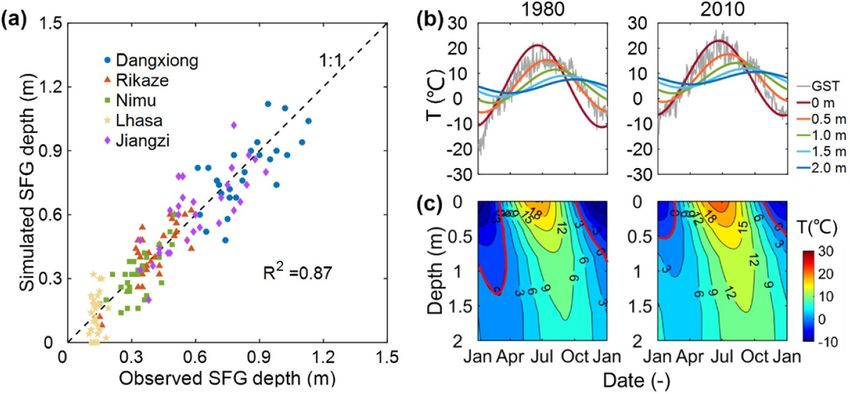
Environ. Res. Lett. 15 (2020) 104081                                                                                          F Ji et al

   Figure 2. (a) Comparison of the simulated SFG depths based on the calibrated model to observations at the five meteorological
   stations from 1980 to 2010. The calibrated DH values are presented in table 1. (b) Temporal dynamics of ground temperature at
   different depths and (c) ground temperature isotherm plots for 1980 and 2010 at Dangxiong station. The gray curves in (b) show
   the measured GST and the other colored curves depict the simulated temperatures at different depths. The red lines in (c) depict
   the 0 ◦ C isotherm; the maximum annual depth of 0 ◦ C isotherm represents the depth of the frozen ground.

river. In total, these two soil types cover 96% of the               (Dangxiong, Jiangzi, Rikaze, Nimu, Lhasa, blue tri-
study area. Most of the soils are seasonally frozen,                 angle marks in figure 1, Climate Center of Tibet).
accounting for about 70% of the entire study area                    Hence, we use all datasets at the ten stations to
(Zou et al, 2017, figure 1). Meadow is the dom-                      adjust the bias associated with the grid-data products
inant vegetation type in the SFG zone (upstream                      (GLDAS and CMIP5). The five stations with SFG
and midstream basins), whereas forest mainly occupy                  depth data were used to calibrate our GT-SFG depth
the downstream perennial unfrozen region in the                      model (described in section 2.2). Because the annual
southeast (Zeng et al 2018). The mean annual total                   snowfall amount is marginal compared with rain-
rainfall amount (based on the rainfall data from                     fall at these stations, the snowfall is not considered
1980 to 2010) gradually decreases from southeast to                  in the model calibration. The details of the five sta-
northwest. The mean annual total rainfall amount                     tions including location, elevation, soil and veget-
in the southeast can reach as high as 1600 mm,                       ation types, mean annual GST, mean annual total
whereas in the northwest, the mean annual total                      rainfall and snowfall amount, calibrated thermal dif-
rainfall amount rarely exceeds 300 mm. Due to the                    fusivity (DH ), and simulation time period are listed
Himalayan collision and post-collision, the YZRB is                  in table 1.
tectonically active with three geological structures:                     To assess the spatial pattern of SFG depth across
Himalayan orogen, Gangdese arc, and Lhasa terrane.                   the entire basin in the historical period (from 1980
The northeastern basin is interspersed by the Bomi-                  to 2010), we employ the spatially resolved daily sur-
Chayu batholith (Yin 2006). The complex geological                   face skin temperature (the temperature on the top
structures, lithology, and thermal conditions con-                   canopy layer, Bense et al 2016, Luo et al 2018)
tribute to numerous geothermal fields in the east of                 products from GLDAS CLSM (Catchment Land Sur-
the basin, which may affect the thermal condition                    face Model, Rodell et al 2003) to drive the GT-SFG
and thus the thickness of frozen ground (including                   depth model. The GLDAS dataset has been success-
SFG and permafrost) in this region (Geothermal and                   fully applied to the QTP for hydrological simulations
Geological Institute, 1991). The spatial distributions               (Qi et al 2018). The utilized GLDAS data have a spa-
of the topographic elevation, soil type, vegetation,                 tial resolution of 0.25◦ × 0.25◦ and span the time
and mean annual total rainfall amount are presented                  period from 1980 to 2010. To project the SFG depth
in supplementary information S1 (available online at                 in the study area under future climate change, we opt
https://stacks.iop.org/ERL/15/104081/mmedia).                        to use the near-surface air temperature (air temperat-
    A total of 10 meteorological stations (figure 1)                 ure measured at a screen-height of 1.5–2 m) products
are located within the YZRB. All stations have recor-                generated by the CCSM4 model developed by the
ded daily GST data for the period from 1980 to                       National Center for Atmospheric Research (NCAR)
2013 (China Meteorological Data Service Center,                      of the United States from the CMIP5 project as the
http://data.cma.cn/en). However, the annual SFG                      input for the GT-SFG depth model. The CCSM4
depth data, i.e. the maximum frozen ground depth                     products have a spatial resolution of 1.25◦ × 0.94◦ .
throughout a year, are only available at five stations               This model is selected because it provides long-term

                                                      3
Environ. Res. Lett. 15 (2020) 104081
Table 1. Geographic location, elevation, soil and vegetation types, mean annual GST, mean annual rainfall and snowfall, calibrated DH values and time periods for the five meteorological stations.
4
Station Longitude [◦ ] Latitude [◦ ] Elevation [m] Soil type Vegetation type GST [◦ C] Rainfall [mm] Snowfall [mm] DH (10–7 m2 · s−1 ) Time period
Dangxiong 91.10 30.48 4200 Sandy loam Meadow 6.5 531.10 17.15 1.23
Jiangzi 89.60 28.92 4040 Loam Meadow 10.2 920.50 26.93 2.03
Rikaze 88.67 29.23 3836 Loam Meadow 11.2 887.04 29.37 1.56 1980–2010
Nimu 90.17 29.43 3809 Loam Meadow 11.6 784.95 11.09 0.44
Lhasa 91.13 29.67 3649 Loam Meadow 12.0 675.12 7.23 3.98
F Ji et alEnviron. Res. Lett. 15 (2020) 104081 F Ji et al
Figure 3. (a) Spatial distribution of SFG depth in 1980; (b) Decadal changes of SFG depth from 1980 to 2010. White areas in
(a) and (b) represent permafrost regions. The values in the lower-left corner denote the basin averages of the SFG depth and
decadal changes (e.g. −0.09 m means differences of SFG depth between 2000 and 1990). These results were computed using
spatially variable DH and (adjusted) GLDAS surface skin temperature datasets with a spatial resolution of 0.25◦ × 0.25◦ .
climate projection up to the year of 2300. We con- time of t [day] based on the annual average GST
sider two typical climate projection scenarios in this T̄0 [◦ C]:
study- ‘RCP 4.5’ and ‘RCP 8.5’ (RCP stands for Rep- [ ]
resentative Concentration Pathways, Moss et al 2008). 2π
T0 = T̄0 + A0 sin (t − φ0 ) (1)
Because our GT-SFG depth model (as described P
later in section 2.2) uses GST as model inputs, we
adjusted the GLDAS surface skin temperature and where A0 [◦ C] is the amplitude of the sinusoidal
CMIP5 near-surface air temperature to approxim- curve and A0 = (T0max − T0min ) /2, with T0max [◦ C]
ate gridded GST based on GST measurement before and T0min [◦ C] representing the maximum and min-
using them to drive the GT-SFG depth model (for imum daily GST; P [day] is the period of the sinus-
details of the data pre-processing, see supplementary oidal function and is defined as 365 days in this study;
information S2). φ0 [day] is the initial phase to run the seasonal tem-
perature changes.
2.2. The GT-SFG depth model The amplitude of the temperature cycle decreases
The GT-SFG depth model estimates SFG depth from with increasing depth as less energy is available to heat
the temporal dynamics of GTs at different soil depths. the soil at deeper locations. Because it takes time for
Annual GSTs are controlled by the energy inputs heat to travel into and out of the soil, there is a time
to the soil surface in response to natural periodic lag C between the sinusoidal temperature curves at
changes in solar radiation. We first employ a sinus- deeper soil depth and at the soil surface, and the time
oidal model (equation (1), Hanks 1992; Hu et al 2016) lag becomes more pronounced with increasing depth
to assess the annual dynamics of GST T0 [◦ C] at the (Hanks 1992). All these changes in soil temperature
5Environ. Res. Lett. 15 (2020) 104081 F Ji et al
Figure 4. Temporal dynamics of simulated basin average SFG depth in the YZRB from 1980 to 2300. The average SFG depths from
1980 to 2005 were calculated based on GLDAS data (black line) and historical data of CMIP5 (green line), whereas those from
2006 to 2300 were computed based on projected climate scenarios of RCP 4.5 and RCP 8.5 (blue and red lines). The shaded areas
show the ranges of average SFG depth accounting for the uncertainties of soil properties. The inset in the lower-left corner shows
the historical and projected basin averages of the minimum daily near-surface air temperature (min NSAT) in the 2 climate
scenarios.
amplitude and time lag affected by soil depth z [m] is for each year and compute the SFG depth as the
described by equation (2): maximum depth of the 0 ◦ C isotherm for each year.
[ ] In addition to the temperature inputs, soil thermal
2π
T (z) = T̄0 + A (A0 , z) · sin (t − φ0 ) − C (z) diffusivity DH largely determine the SFG depth
P (a sensitivity analysis of the SFG depth to DH is shown
(2)
in supplementary information S3). In the following
where T (z) [◦ C] and A (A0 , z) [◦ C] are the soil tem-
analysis, we first calibrate the GT-SFG depth model
perature and amplitude at the depth of z [m]. C (z)
for each individual station with measured SFG depth
[−] is the time lag as a function of depth of z [m].
data, then apply this model to the entire YZRB using
The variables A and C are linked to depth (z) by
GLDAS and CMIP5 data as model input. It is note-
the following formulas:
worthy that this model is not applicable to permafrost
A (A0 , z) = A0 · e− d
z
(3) due to different heat transport mechanisms in SFG
and permafrost: only one-side freezing from surface
downwards in SFG but two-side freezing from sur-
z face downwards and from permafrost table upwards
C (z) = (4) in permafrost (Thomas et al 2009).
d
where d [m] is the characteristic damping depth that
is dependent on soil thermal diffusivity DH [m2 · s−1 ]. 2.3. Soil spatial variability
We incorporate the spatial variability of soil thermal
√ diffusivity DH into the GT-SFG depth model by estab-
P · τ · DH lishing the relationship between DH and soil wet-
d= (5)
π ness condition for different soil types based on the
calibrated DH and the local conditions at the met-
The symbol τ is the time step factor (86 400 s · day−1 ). eorological stations. For soil wetness, as soil mois-
Integrating equations (3)–(4) to equation (2) ture is often considered to be among the most
yields: difficult hydrologic component to determine and
[ ] varies drastically with soil depth, we use the easy-
2π z
T (z) = T̄0 + A0 · e− d · sin
z
(t − φ0 ) − (6) to-measure mean annual total rainfall amount as
P d
a proxy to soil wetness condition (previous studies
This model uses daily GST as inputs for have demonstrated that soil moisture and rainfall are
equation (6) and computes the daily GTs at differ- closely correlated in this region, e.g. Bi et al 2016).
ent depths. We then derive the GT isotherm plots The soil wetness is thus represented by the linearly
6Environ. Res. Lett. 15 (2020) 104081 F Ji et al
scaled mean annual rainfall (R) ranging from 0 to 1, in figure 2(a). As an example, the daily dynamics of
with larger scaled R indicating wetter soil and vice GT at different depths (from ground surface to 2 m
versa. Loam and sandy loam are the two dominant depth which corresponds to the maximum observed
soil types covering 96% of the study area (supple- SFG depth) and the GT isotherm plots at Dangx-
mentary information S1), hence we simplify the soil iong station for 1980 and 2010 are shown in fig-
types in the basin into these two major categories. ures 2(b) and (c), indicating a SFG depth of ∼1.5 m
Based on the calibrated DH and local conditions at and ∼0.5 m in the year of 1980 and 2010, respect-
the five meteorological stations, a linear relationship ively. The simulated time series of the SFG depth at
between soil thermal diffusivity and soil wetness is the five meteorological stations shows good agree-
derived for loam and sandy loam, respectively (for ment with observations (supplementary information
details, see supplementary information S4). We then S6). These results indicate that, despite the simpli-
apply the linear models to the entire basin accord- city, the proposed model calculates reasonable SFG
ing to the site-specific soil type and scaled rainfall depths using GST as major model input. It appears
amount (R). that there exists relatively large discrepancy between
Note that soil moisture is also affected by soil type. simulated and observed SFG depths at the Lhasa sta-
Due to different soil water retention characteristics, tion. We attribute this discrepancy to the influence
soil type affects the rainwater infiltration, soil water of land use: The Lhasa station is located in urban
holding capacity, and the drainage dynamics during area, while the other four stations are located in nat-
and after rainfall. Under similar wetness condition, ural regions covered by meadow. The urban land use
rainwater infiltrates faster into coarse soil with larger type at the Lhasa station hinders the heat transport
infiltration capacity than fine soil and thus increases through the soil profile, leading to shallower SFG
the soil water content. But immediately after rainfall, depths with smaller variability. But for the regional
coarse soil also evaporates and drains at higher rates, scale analysis (section 3.2 and 3.3), we have not spe-
which reduce soil water content. Infiltration, evap- cifically considered the effects of urban land use type,
oration and drainage jointly determine the dynamics as the YZRB is a highly underdeveloped region with
of soil water content. These processes are affected by the urban land use type only occupying less than 1%
internal and external factors such as soil type, topo- of the total basin (Fang and Li 2015).
graphy and precipitation patterns. The consideration
of these detailed soil water dynamics tremendously 3.2. Historical SFG spatiotemporal patterns
increases the complexity of this study. Hence, we opt This section investigates the spatiotemporal pat-
to use the (scaled) mean annual rainfall amount as terns of SFG depth in the entire YZRB for the
a proxy for soil water content in this study for the historical time period (1980–2010) using (adjus-
purpose of regional scale study. It is also noteworthy ted) GLDAS surface skin temperature data as model
that the SFG zone in our study area is dominated by inputs. The spatial distribution of the SFG depth in
one single vegetation type- meadow which occupies 1980 (figure 3(a)) indicates a clear spatial pattern:
90% of the total SFG area (supplementary inform- the seasonally frozen soil is mostly located in the
ation S1). This allows us to simplify the analysis by northwest of the basin with SFG depth ranging from
neglecting the effects of vegetation variability. But 1.5 m to 4 m, whereas the SFG depth in the south-
we acknowledge that vegetation type and soil organic east is less than 1 m with perennial unfrozen area
carbon (SOC) content are important factors influ- in the southeast (to the south of the Linzhi station).
encing the soil thermal diffusivity and thus the SFG Figure 3(b) depicts three examples of the differences
depth in regions with spatially variable vegetation between the SFG depth in different years. It reflects a
distribution. We provide a protocol to incorporate greater decrease in seasonally frozen soil depth in the
the impacts of vegetation type and SOC on the SFG northwest than in the southeast (figure 3(b), a negat-
depths into the GT-SFG depth model based on the ive value denoting a decreasing SFG depth). This spa-
links between soil thermal diffusivity, vegetation type tial pattern is largely due to more intense increases in
and SOC. The details of this protocol are presented in the surface skin temperature in the northwest (sup-
supplementary information S5. plementary information S7). The spatial variability
of soil properties also contributed to the spatial pat-
3. Results tern of SFG depth (higher soil thermal diffusivity in
the northwest compared with south of this region,
3.1. Calibrating the GT-SFG depth model supplementary information S8). Despite annual fluc-
This section presents the calibration results of the tuations, the average SFG depth across the entire
GT-SFG depth model based on the five meteorolo- basin (excluding the unfrozen zone in the southeast)
gical stations within the YZRB from 1980 to 2010. decreases at a rate of 2.50 cm · a−1 for the time period
The calibrated DH values for the five meteorolo- of 1980–2010 (shown in figure 4 in section 3.3). Our
gical stations are presented in table 1. A compar- simulated SFG depths are also confirmed by the mod-
ison of simulated and observed SFG depth at the five eling results based on the semi-analytical Stefan’s
meteorological stations from 1980 to 2010 is shown method that relates the SFG depth to GST and soil
7Environ. Res. Lett. 15 (2020) 104081 F Ji et al
thermal properties. Details of the Stefan’s method The proposed modeling framework provides a
and its comparison to our GT-SFG depth model are simple yet robust approach to estimate the temporal
shown in supplementary information S9. dynamics of vertical temperature distribution and
SFG depth. This model is particularly useful in data-
scarce regions (such as the QTP in this study) as
3.3. Projected SFG dynamics under climate change
it requires minimum model input (i.e. the surface
We employed the (adjusted) near-surface air temper-
GT, which is nearly universally available over the
ature data generated by the CCSM4 model in two pro-
globe) compared with other physically-based mod-
jected climate change scenarios (RCP 4.5 and RCP
els. In addition, the reduced computational burden
8.5) as model inputs for the GT-SFG depth model
allows the estimation of the depth at the regional scale
to estimate future changes of the SFG depth in the
(e.g. over 10 000 km2 ) spanning long time periods
YZRB. The simulated basin average SFG depths show
(e.g. decades). The temporally evolving spatial distri-
continuing negative trends in both RCP 4.5 and RCP
butions of the SFG depth at the regional scale will
8.5 climate scenarios (figure 4). The shaded blue and
be useful for constraining more sophisticated phys-
red areas in figure 4 shows the ranges of average SFG
ically based numerical models that consider specific-
depth under RCP 4.5 and RCP 8.5 scenarios for the
ally water flow and heat transport in multi-phase
period 2006 to 2300 accounting for the uncertain-
media in cold regions. More field data with increased
ties of soil properties as described in supplement-
spatial density for a longer time period will further
ary information S4. Particularly, we observed a lin-
constrain our model, but our estimates provide an
ear decrease of the average SFG depth (log scale) with
important basis for the evaluation of the hydrological
time in the RCP 8.5 scenario (log10 (SFG) = 0.23–
cycles (e.g. seasonal groundwater recharge and sur-
0.0047 · T, R2 = 0.85, with T denoting the elapsed
face water-groundwater exchanges) in cold regions
years since 1980) and that the average SFG depth
under changing climatic conditions.
tends to level off at ∼0.1 m after 2180 in the RCP
8.5 scenario, implying that most areas in current SFG
zone are projected to no longer have SFG in the future Acknowledgments
due to climate warming. The basin average of the
minimum near-surface air temperature throughout a This work was supported by the National Natural Sci-
year is projected to exceed 0 ◦ C after 2180 in the RCP ence Foundation of China (grants nos. 41861124003
8.5 scenario (see the inset of figure 4). In addition to and 91747204). Additional support was provided by
the CCSM4 model, we also computed the future SFG the State Environmental Protection Key Laboratory
depth using near-surface air temperature products of Integrated Surface Water-Groundwater Pollution
generated by 8 additional GCMs (General Circulation Control of China. We are grateful to David N Lerner,
Models) from CMIP5. The results confirm the negat- Yuqing Feng and Yu Feng for helpful discussion and
ive trend of the SFG depth, despite the large range of assistance.
the SFG depth computed by different GCMs (supple-
mentary information S10). Data availability statement
The data that support the findings of this study
4. Summary and conclusions
are openly available at the following URL/DOI:
https://hydro1.gesdisc.eosdis.nasa.gov/data/GLDAS/
We propose a semi-empirical GT-SFG depth model
GLDAS_CLSM025_D.2.0 and https://esgf-
to investigate the spatiotemporal dynamics of the
node.llnl.gov/projects/esgf-llnl.
SFG depth in the YZRB on the QTP via the simula-
tion of long-term time series of GT at different soil
depths. This model was first calibrated using ground ORCID iDs
station observations and then applied to the entire
basin using data assimilation products of GLDAS Linfeng Fan https://orcid.org/0000-0002-5776-
(1980–2010) and GCM projections (2006–2300) to 1738
assess the spatiotemporal patterns of the SFG depth Chunmiao Zheng https://orcid.org/0000-0001-
under climate change. The results suggest that the 5839-1305
average SFG depth in YZRB has decreased at a rate
of 2.50 cm · a−1 from 1980 to 2010, with more severe References
decrease in the northwestern upstream regions than
Bense V F, Read T and Verhoef A 2016 Using distributed
in the southeastern downstream regions. The future temperature sensing to monitor field scale dynamics of
projections indicate that the current SFG depth in the ground surface temperature and related substrate heat flux
YZRB will continue to decrease in response to future Agric. For. Meteorol. 220 207–15
warming and may disappear by 2180 under the RCP Bi H, Ma J, Zheng W and Zeng J 2016 Comparison of soil
moisture in GLDAS model simulations and in situ
8.5 scenario (if not considering the transition of per- observations over the Tibetan Plateau J. Geophys. Res. 121
mafrost to SFG). 2658-78
8Environ. Res. Lett. 15 (2020) 104081 F Ji et al
Evans S G and Ge S 2017 Contrasting hydrogeologic responses to Qi W, Liu J and Chen D 2018 Evaluations and improvements of
warming in permafrost and SFG hillslopes Geophys. Res. GLDAS2.0 and GLDAS2.1 forcing data’s applicability for
Lett. 44 1803-13 basin scale hydrological simulations in the Tibetan Plateau
Fang C and Li G 2015 Particularities, gradual patterns and J. Geophys. Res. 123 13128–48
countermeasures of new-type urbanization in Tibet, China Qin Y, Chen J, Yang D and Wang T 2018 Estimating seasonally
Bull. Chin. Acad. Sci. 30 294–305 frozen ground depth from historical climate data and site
Ge J M, Huang J, Su J and Bi J R 2011 Exchange of groundwater measurements using a Bayesian model Water Resour. Res.
and surface-water mediated by permafrost response to 54 4361–75
seasonal and long term air temperature variation Geophys. Rawlins M A, Nicolsky D J, Mcdonald K C and Romanovsky V E
Res. Lett. 38 14402 2013 Simulating soil freeze/thaw dynamics with an
Geothermal and Geological Institute, Tibet Autonomous Region improved pan-Arctic water balance model J. Adv. Model.
Geological and Mineral Exploration and Development Earth Syst. 5 659–75
Bureau 1991 Geothermal resource regionalisation in Tibet Rodell M, Houser P R, Jambor U, Gottschalck J, Mitchell K,
Autonomous Region (Internal report) Meng C, Arsenault K, Cosgrove B, Radakovich J and
Gouttevin I, Krinner G, Ciais P, Polcher J and Legout C 2012 Bosilovich M 2003 The global land data assimilation system
Multi-scale validation of a new soil freezing scheme for a Bull. Amer. Meteor. Soc. 85 381-94
land-surface model with physically-based hydrology The Stefan J 1891 Über die Theorie der Eisbildung, insbesondere
Cryosphere 6 407–30 über die Eisbildung im Polarmee. Ann. Phys. Chem.
Guo D and Wang H 2016 CMIP5 permafrost degradation 278 269–86
projection: acomparison among different regions J. Geophys. Taylor K E, Stouffer R J and Meehl G A 2012 An overview of
Res. 121 4499–517 CMIP5 and the experiment design Bull. Am. Meteorol. Soc.
Hanks R J 1992 Applied Soil Physics 2nd edn (Berlin: Springer) 93 485–98
Hansson K, Šimůnek J, Mizoguchi M, Lundin L C and Thomas H R, Cleall P, Li Y-C, Harris C and Kern-Luetschg M
and Genuchten M T V 2004 Water flow and heat transport 2009 Modelling of cryogenic processes in permafrost and
in frozen soil Vadose Zone J. 3 527–33 seasonally frozen soils Géotechnique 59 173–84
Hu G, Zhao L, Wu X, Li R, Wu T, Xie C, Qiao Y, Shi J, Li W and Voss C I and Provost A M (2010), SUTRA: A model for
Cheng G 2016 New Fourier-series-based analytical solution saturated-unsaturated variable density groundwater flow
to the conduction–convection equation to calculate soil with solute or energy transport. Version 2.2,
temperature, determine soil thermal properties, or estimate Water-Resources Investigations Report 02−4231: U.S. Geol.
water flux Int. J. Heat Mass Transf. 95 815–23 Surv., 291p.
Jin H, He R, Cheng G, Wu Q, Wang S, Lü L and Chang X 2009 Yang D, Kane D L, Hinzman L D, Zhang X, Zhang T and Ye H
Changes in frozen ground in the source area of the yellow 2002 Siberian Lena River hydrologic regime and recent
river on the Qinghai–Tibet Plateau, China, and their change J. Geophys. Res. 107 ACL 14-1-ACL 14–10
eco-environmental impacts Environ. Res. Lett. 4 045206 Yin A 2006 Cenozoic tectonic evolution of the Himalayan orogen
Jumikis A R 1977 Thermal Geotechnics (New Brunswick, New as constrained by along-strike variation of structural
Jersey: Rutgers University Press) geometry, exhumation history, and foreland sedimentation
Kudryavtsev V A, Garagula L S, Kondrat’yeva K A and Earth-Sci. Rev. 76 1–131
Melamed V G 1977 Fundamentals of Frost Forecasting in Zeng C, Zhang F, Lu X, Wang G and Gong T 2018 Improving
Geological Engineering Investigations. Draft Translation 606 sediment load estimations: the case of the Yarlung Zangbo
(Hanover, NH: U.S. Army CCREL) River (the upper Brahmaputra, Tibet Plateau) Catena
Luo D, Jin H, Marchenko S S and Romanovsky V E 2018 160 201–11
Difference between near-surface air, land surface and ground Zhang Y, Cheng G, Li X, Jin H, Yang D, Flerchinger G N, Chang X,
surface temperatures and their influences on the frozen Bense V F, Han X and Liang J 2017 Influences of frozen
ground on the Qinghai-Tibet Plateau Geoderma 312 74–85 ground and climate change on hydrological processes in an
Moss R, Babiker W, Brinkman S, Calvo E, Carter T and Edmonds Alpine watershed: A case study in the upstream area of the
J et al Intergovernmental Panel on Climate Change Hei’he River, Northwest China Permafr. Periglac. Process.
Secretariat (IPCC) 2008 Towards New Scenarios for the 28 420–32
Analysis of Emissions: Climate Change, Impacts and Zhao L, Ping C-L, Yang D, Cheng G, Ding Y and Liu S 2004
Response Strategies Geneva, Switzerland. Changes of climate and SFG over the past 30 years in
Moss R et al 2010 The next generation of scenarios for climate Qinghai–Xizang (Tibetan) Plateau, China Glob. Planet.
change research and assessment Nature 463 747–56 Change 43 19–31
Pang Q, Zhao L, Li S and Ding Y 2011 Active layer thickness Zhong L, Ma Y, Fu Y, Pan X, Hu W, Su Z, Salama M S and Feng L
variations on the Qinghai–Tibet Plateau under the scenarios 2014 Assessment of soil water deficit for the middle reaches
of climate change Environ. Earth Sci. 66 849–57 of Yarlung-Zangbo River from optical and passive
Peng X, Zhang T, Frauenfeld O W, Wang K, Cao B, Zhong X, Su H microwave images Remote Sens. Environ. 142 1–8
and Mu C 2017 Response of seasonal soil freeze depth to Zou D et al 2017 A new map of permafrost distribution on the
climate change across China The Cryosphere 11 1059–73 Tibetan Plateau The Cryosphere 11 2527–42
9You can also read