Study of the tidal dynamics of the Korea Strait using the extended Taylor method
←
→
Page content transcription
If your browser does not render page correctly, please read the page content below
Ocean Sci., 17, 579–591, 2021
https://doi.org/10.5194/os-17-579-2021
© Author(s) 2021. This work is distributed under
the Creative Commons Attribution 4.0 License.

Study of the tidal dynamics of the Korea Strait using
the extended Taylor method
Di Wu1 , Guohong Fang1,2 , Zexun Wei1,2 , and Xinmei Cui1,2
1 First
      Institute of Oceanography, Ministry of Natural Resources, Qingdao, 266061, China
2 Laboratory for Regional Oceanography and Numerical Modeling, Pilot National Laboratory for Marine Science
and Technology, Qingdao, 266237, China

Correspondence: Guohong Fang (fanggh@fio.org.cn)

Received: 1 September 2020 – Discussion started: 28 September 2020
Revised: 17 February 2021 – Accepted: 7 March 2021 – Published: 23 April 2021

Abstract. The Korea Strait (KS) is a major navigation pas-         1   Introduction
sage linking the Japan Sea (JS) to the East China Sea and
Yellow Sea. Almost all existing studies of the tides in the KS
employed either data analysis or numerical modelling meth-         The Korea Strait (KS, also called the Tsushima Strait) con-
ods; thus, theoretical research is lacking. In this paper, we      nects the East China Sea (ECS) to the southwest and the
idealize the KS–JS basin as four connected uniform-depth           Japan Sea (the JS, also called the East Sea, or the Sea of
rectangular areas and establish a theoretical model for the        Japan) to the northeast. It is the main route linking the JS to
tides in the KS and JS using the extended Taylor method.           the ECS and the Yellow Sea and is thus an important pas-
The model-produced K1 and M2 tides are consistent with             sage for navigation. The strait is located on the continental
the satellite altimeter and tidal gauge observations, especially   shelf, and it has a length of approximately 350 km, a width of
for the locations of the amphidromic points in the KS. The         250 km and an average water depth of approximately 100 m.
model solution provides the following insights into the tidal      The JS, which is adjacent to the KS, is a deep basin that
dynamics. The tidal system in each area can be decomposed          has an average depth of approximately 2000 m and a depth
into two oppositely travelling Kelvin waves and two families       of more than 3000 m at its deepest part. A steep continen-
of Poincaré modes, with Kelvin waves dominating the tidal          tal slope separates the KS and the JS, and it presents abrupt
system. The incident Kelvin wave can be reflected at the con-      depth and width changes (Fig. 1). Such topographic charac-
necting cross section, where abrupt increases in water depth       teristics create the unique tidal waves that occur in the KS.
and basin width occur from the KS to JS. At the connecting            Ogura (1933) first conducted a comprehensive study of
cross section, the reflected wave has a phase-lag increase rel-    the tides in the seas adjacent to Japan using data from the
ative to the incident wave of less than 180◦ , causing the for-    tidal stations along the coast and gained a preliminary un-
mation of amphidromic points in the KS. The above phase-           derstanding of the characteristics of the tides, including am-
lag increase depends on the angular velocity of the wave and       phidromic systems in the KS. Since then, many researchers
becomes smaller as the angular velocity decreases. This de-        have investigated the tides in the strait via observations
pendence explains why the K1 amphidromic point is located          (Odamaki, 1989a; Matsumoto et al., 2000; Morimoto et al.,
farther away from the connecting cross section in comparison       2000; Teague et al., 2001; Takikawa et al., 2003) and numer-
to the M2 amphidromic point.                                       ical simulations (Fang and Yang, 1988; Kang et al., 1991;
                                                                   Choi et al., 1999; Book et al., 2004). The results of these
                                                                   studies show consistent structures of the tidal waves in the
                                                                   KS. Figure 2 displays the distributions of the K1 and M2 tidal
                                                                   constituents based on the global tidal model DTU10, which
                                                                   is based on satellite altimeter observations (Cheng and An-
                                                                   dersen, 2011). The figures show that the amplitudes of the

Published by Copernicus Publications on behalf of the European Geosciences Union.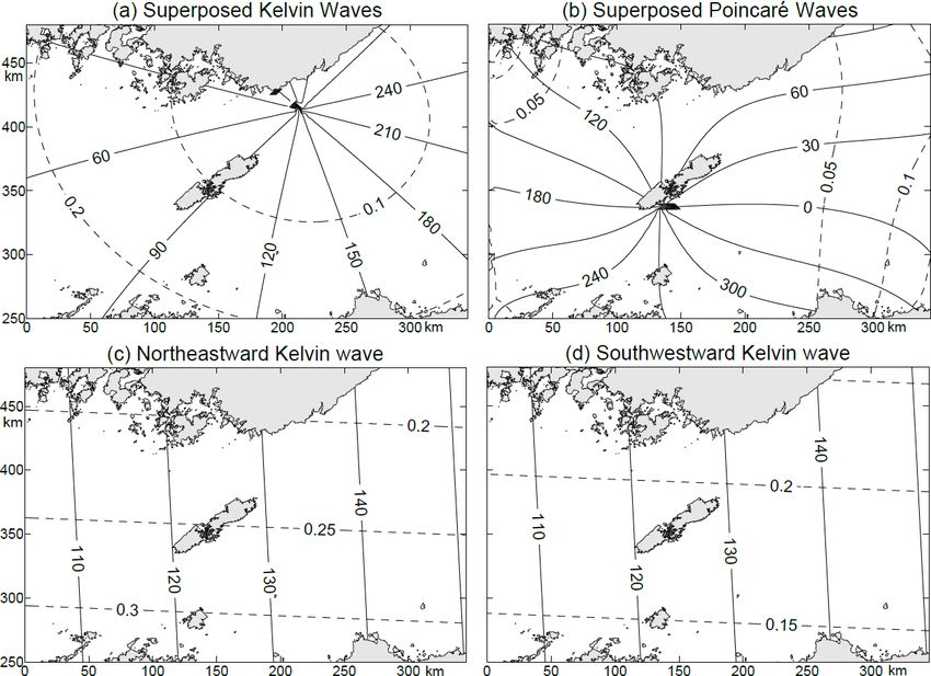
580 D. Wu et al.: Study of the tidal dynamics of the Korea Strait
2 The extended Taylor method and its application to
multiple rectangular areas
The Taylor problem is a classic tidal dynamic problem (Hen-
dershott and Speranza, 1971). Taylor (1922) first presented a
theoretical solution for tides in a semi-infinite rotating rect-
angular channel of uniform depth to explain the formation
of amphidromic systems in gulfs and applied the theory to
the North Sea. The classic Taylor problem was subsequently
improved by introducing frictional effects (Fang and Wang,
1966; Webb, 1976; Rienecker and Teubner, 1980) and open-
boundary conditions (Fang et al., 1991) to study tides in mul-
tiple rectangular basins (Jung et al., 2005; Roos and Schut-
telaars, 2011; Roos et al., 2011) as well as to solve tidal dy-
namics in a strait (Wu et al., 2018).
The method initiated by Taylor and developed afterwards
is called the extended Taylor method (Wu et al., 2018). This
method is especially useful in understanding the tidal dy-
namics in marginal seas and straits because the tidal waves
in these sea areas can generally be represented by combina-
tions of the Kelvin waves and Poincaré waves/modes (e.g.
Taylor, 1922; Fang and Wang, 1966; Hendershott and Sper-
anza, 1971; Webb, 1976; Fang et al., 1991; Carbajal, 1997;
Figure 1. Map of the Korea Strait and its neighbouring areas. (TTS: Jung et al., 2005; Roos and Schuttelaars, 2011; Roos et al.,
Tartar Strait; SYS: Soya Strait; TGS: Tsugaru Strait; KS: Korea 2011; Wu et al., 2018).
Strait; ECS: East China Sea). Isobaths are in metres (based on
ETOPO1 from US National Geophysical Center). 2.1 Governing equations and boundary conditions for
multiple rectangular areas
diurnal tides are smaller than the semidiurnal tides. The peak A sketch of the model geometry is shown in Fig. 3, and it
amplitude of the semidiurnal tide appears on the south coast consists of a sequence of J rectangular areas with length Lj ,
of South Korea, and lower amplitudes occur along the south- width Wj and uniform depth hj for the j th rectangular area
ern shore of the strait from the ECS to the JS. Distinguishing (denoted as Areaj , j = 1, . . . , J ). For convenience, the shape
features include (1) K1 and M2 amphidromic points in the of the study region shown in Fig. 3 is the same as that for the
strait that appear in the northeast part of the KS close to the idealized KS–JS basin, which will be described in the next
southern coast of the Korean Peninsula and (2) the M2 am- section. In particular, Area1 represents the KS, which is our
phidromic point appears further northeast and closer to the focus area in this study.
shelf break relative to the K1 tide. Consider a tidal wave of angular velocity σ and typical el-
However, almost all previous studies have employed either evation amplitude H . We assume H / h
1, and the conser-
data analysis or numerical modelling methods; thus, theoret- vation of momentum and mass leads to the following depth-
ical research is lacking. In particular, the existence of am- averaged linear shallow water equations on the f plane:
phidromic points in the northeast KS for both diurnal and
∂ ũj ∂ ζ̃j
semidiurnal tides has not been explained based on geophys- ∂t − fj υ̃j = −g ∂x − γj ũj
ical dynamics. In this paper, we intend to establish a theo- ∂ υ̃j ∂ ζ̃
∂t + fj ũj = −g ∂yj − γj υ̃j , (1)
retical model for the K1 and M2 tides in the KS–JS basin
∂ ζ̃j
h
∂ ũ ∂ υ̃
i
= −hj ∂xj + ∂yj
using the extended Taylor method. The model idealizes the
∂t
KS–JS basin into three connected uniform-depth rectangular
where x and y are coordinates in the longitudinal (along-
areas, with the effects of bottom friction and Coriolis force
channel) and transverse (cross-channel) directions; t repre-
included in the governing equations and with the observed
sents time; ũj and υ̃j represent the depth-averaged flow ve-
tides specified as open-boundary conditions. The extended
locity components in the x and y directions, respectively,
Taylor method enables us to obtain semi-analytical solutions
with the subscript j indicating the area number; ζ̃j represents
consisting of a series of Kelvin waves and Poincaré modes.
the free surface elevation above the mean level; γj represents
the frictional coefficient, which is taken as a constant for each
tidal constituent in each area; g = 9.8 ms−2 represents the
acceleration due to gravity; and fj represents the Coriolis
Ocean Sci., 17, 579–591, 2021 https://doi.org/10.5194/os-17-579-2021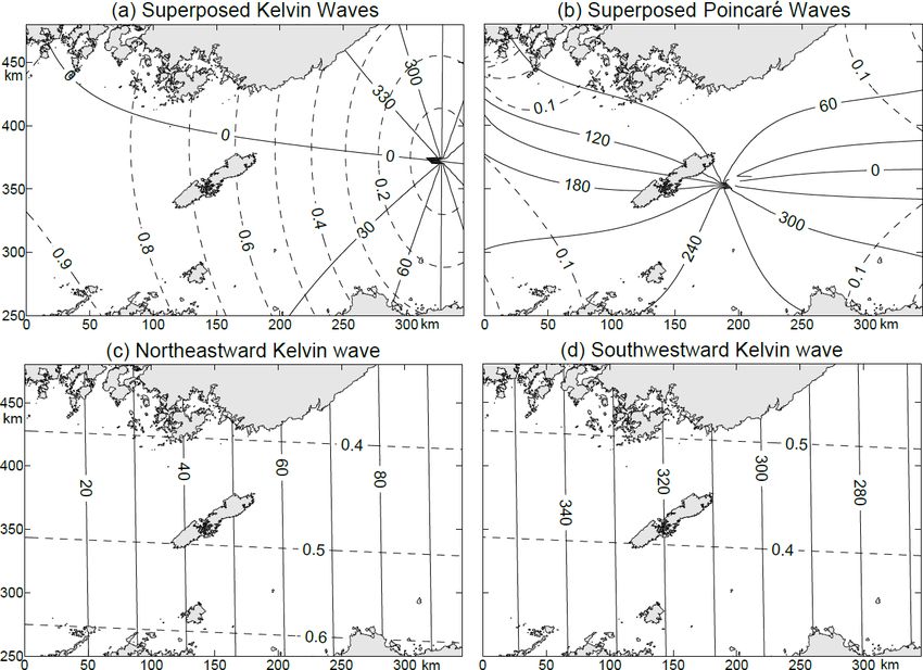
D. Wu et al.: Study of the tidal dynamics of the Korea Strait 581
Figure 2. Tidal charts of the KS and its neighbouring areas based on DTU10 (Cheng and Andersen, 2011) for the (a) K1 tide and (b) M2
tide. Solid lines represent the Greenwich phase lag (in degrees), and dashed lines represent amplitude (in metres).
Eq. (1) can be reduced as follows:
g ∂ζj
µj + i uj − νj υj = − σ ∂x
∂ζ
µj + i υj + νj uj = − σg ∂yj , (3)
h i
ζj = ihj ∂uj + ∂υj
σ ∂x ∂y
in which
γj fj
Figure 3. Model geometry. µj = and νj = . (4)
σ σ
Provided that the j th rectangular area, denoted as Areaj ,
parameter, which is also taken as a constant based on the av- has a width of Wj , has a length of Lj and ranges from x = lj
erage of the concerned area. The equations in Eq. (1) for each to x = lj +1 (lj +1 = lj + Lj ) in the x direction and from y =
j are two-dimensional linearized shallow water equations on wj,1 to y = wj,2 (wj,2 = wj,1 + Wj ) in the y direction, the
an f plane with momentum advection neglected. For any j , boundary conditions along the sidewalls within x ∈ [lj , lj +1 ]
the equations are the same as those used in the work of Tay- are taken as follows:
lor (1922) except that bottom friction is now incorporated,
such as in Fang and Wang (1966), Webb (1976) and Rie- υj = 0 at y = wj,1 and y = wj,2 . (5)
necker and Teubner
(1980).
When a monochromatic wave is Along the cross sections, such as x = lj , various choices
considered, ζ̃j , ũj , υ̃j can be expressed as follows: of boundary conditions are applicable depending on the prob-
lem:
ζ̃j , ũj , υ̃j = Re ζj , uj , υj eiσ t ,
(2)
uj = 0, (6)
where Re stands for the real part of the complex quantity if the cross section is a closed boundary;
that follows; ζj , uj , υj are referred to as complex ampli-
√ s
tudes of ζ̃j , ũj , υ̃j , respectively; i ≡ −1 is the imaginary g
uj = ± ζj , (7)
unit; and σ is the angular velocity of the wave. For this wave, 1 − iµj hj
https://doi.org/10.5194/os-17-579-2021 Ocean Sci., 17, 579–591, 2021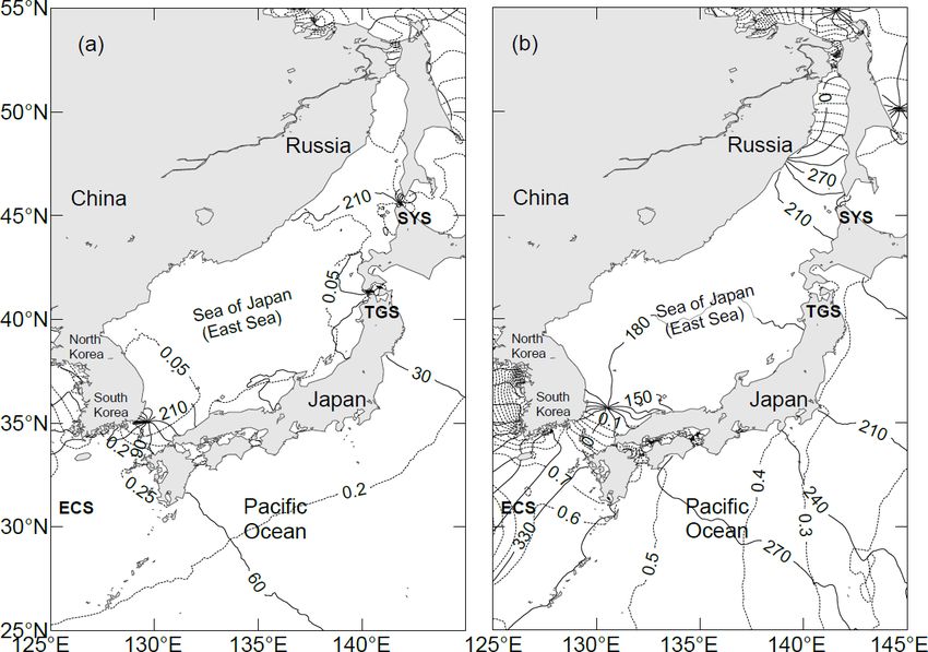
582 D. Wu et al.: Study of the tidal dynamics of the Korea Strait
if the free radiation in the positive/negative x direction occurs where αj , βj , rj,n and sj,n are equal to the following:
on the cross section; νj
αj = 1/2 kj , (14)
1 − iµj
ζj = ζ̂j , (8) 1/2
βj = 1 − iµj kj , (15)
nπ
rj,n = , (16)
if the tidal elevation is specified as ζ̂j along the cross section; Wj
and
and
1
2 2
ζj = ζj +1 ,
(9) sj,n = rj,n + αj2 − βj2 , (17)
uj hj = uj +1 hj +1 ,
p
in which kj = σ/cj is the wave number, with cj = ghj
being the wave speed of the Kelvin wave in the absence
if the cross section is a connecting boundary of the areas j
of friction. The parameters sj,n in Eq. (17) are of funda-
and j + 1, with each having a different uniform depth of hj
mental importance in determining the characteristic of the
and hj +1 .
Poincaré modes. If Re(βj2 − αj2 )1/2 < π/Wj , all Poincaré
Equation (9) is matching conditions accounting for sea
modes are bound in the vicinity of the open, connecting or
level continuity and volume transport continuity. The indi-
closed cross sections (see Fang and Wang, 1966; Hender-
vidual Eqs. (6) to (9), or their combination, may be used as
shott and Speranza, 1971, for an absence of friction), while if
boundary conditions for the cross sections. The relationship
Re(βj2 − αj2 )1/2 > nπ/Wj , the nth and lower-order Poincaré
between uj and ζj shown in Eq. (7) is based on the solu-
modes are propagating waves. In the present study, the in-
tion for progressive Kelvin waves in the presence of friction,
equality Re(βj2 − αj2 )1/2 < π/Wj holds for all rectangular
which will be given in Eqs. (10) and (11) below.
areas shown in Fig. 3, so that all Poincaré modes in the
present study appear in a bound form. The parameter sj,n
2.2 General solution has two complex values for each n, and here we choose the
one that has a positive real part. To satisfy the equations in
For the j th rectangular area, that is, for x[lj , lj +1 ] and Eq. (3), (Aj,n , Bj,n , Cj,n , Dj,n ) and (A0j,n , Bj,n
0 , C 0 , D0 )
j,n j,n
y[wj,1 , wj,2 ], the governing equations in Eq. (3) only have should be as follows:
the following four forms satisfying the sidewall boundary h 2 i
condition of Eq. (5) (see for example Fang et al., 1991): µj + i + νj2 rj,n sj,n
Aj,n = 2 2 sj,n , (18)
µj + i rj,n + νj2 sj,n
2
υj,1 = 0,
νj µj + i αj2 − βj2
uj,1 = −aj exp αj y + iβj x − lj , (10)
β Bj,n = 2 2 , (19)
ζj,1 = σj hj aj exp αj y + iβj x − lj ; + νj2 sj,n
2
µj + i rj,n
υj,2 = 0, Cj,n = rj,n − sj,n Aj,n , (20)
uj,2 = bj exp −αj y − iβj x − lj , (11)
β Dj,n = −sj,n Bj,n , (21)
ζj,2 = σj hbj exp −αj y − iβj x − lj ;
P∞ A0j,n = −Aj,n , (22)
υ j,3 = n=1 κ j,n sin r j,n y exp −s j,n x − l j , 0
P∞ Bj,n = Bj,n , (23)
u = κ
j,3 n=1 j,n A j,n cos rj,n y + B j,n sin r j,n y
0
exp −sj,n x − lj , (12) Cj,n = Cj,n , (24)
ihj X∞
ζj,3 =
κ C cos rj,n y + D1,n sin rj,n y
n=1 j,n j,n and
σ
exp −sj,n x − lj ; 0
Dj,n = −Dj,n . (25)
Equations (10) and (11) represent Kelvin waves propagat-
and
ing in the −x and x directions, respectively; and Eqs. (12)
and (13) represent two families of Poincaré modes bound
υj,4 = ∞
P
sin rj,n y exp −sj,n lj +1 − x ,
n=1 λj,n along the cross sections x = lj and lj +1 in the j th rectan-
P∞ 0 0 gular area, respectively. The coefficients (aj , bj , κj,n , λj,n )
uj,4 = n=1 λj,n Aj,ncos rj,n y + Bj,n sin rj,n y
determine amplitudes and phase lags of Kelvin waves and
exp −sj,n lj +1 − x , (13)
ihj X∞ Poincaré modes. These coefficients must be chosen to satisfy
0 0
ζj,4 =
λ
n=1 j,n
Cj,n cos rj,n y + Dj,n sin rj,n y the boundary conditions, preferably using the collocation ap-
σ
exp −sj,n lj +1 − x , proach.
Ocean Sci., 17, 579–591, 2021 https://doi.org/10.5194/os-17-579-2021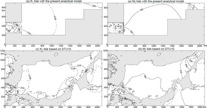
D. Wu et al.: Study of the tidal dynamics of the Korea Strait                                                                             583

2.3    Defant’s collocation approach

The collocation approach was first proposed by Defant in
1925 (see Defant, 1961) and is convenient in determining
the coefficients (aj , bj , κj,n , λj,n ). In the simplest case, that
is, if the model domain contains only a single rectangular
area, then J = 1 and the index j has only one value: j = 1,
the calculation procedure can be as follows. First, we trun-
cate each of the two families of Poincaré modes in Eqs. (12)
and (13) at the N1 th order so that the number of undeter-
mined coefficients for two families of Poincaré modes is 2N1
and the total number of undetermined coefficients (plus those
for a pair of Kelvin waves) is thus 2N1 + 2. To determine
these unknowns, we take equally spaced N1 + 1 dots, which
are called collocation points, located at y = w1,1 + 2(NW1 1+1) ,
          3W1                          1 +1)W1
w1,1 + 2(N  1 +1)
                  , . . . , w1,1 + (2N
                                     2(N1 +1) on both cross sections
x = l1 and l2 . At these points, one of the boundary condi-
tions given by Eqs. (6) to (8) should be satisfied, which yields
2N1 + 2 equations. By solving this system of equations, we
can obtain 2N1 + 2 coefficients (a1 , b1 , κ1,n , λ1,n ). Because       Figure 4. Idealized model domain fitting the Korea Strait and Japan
the high-order Poincaré modes, which have great values of n             Sea. The dashed line represents an open boundary, and the solid
and s1,n in Eqs. (12) and (13), decay from the boundary very            lines represent closed boundaries. A, B, . . . , M indicate the locali-
quickly, it is generally necessary to retain only a few lower-          ties of the points used in Fig. 6 for model–observation comparison.
                                                                        Numbered red dots are tidal gauge stations where the observed har-
order terms. In the above single-rectangle case, the spacing
                                                                        monic constants are used for model validation in Table 2.
of collocation points is equal to 1y = W1 /(N1 + 1).
   For J > 1, that is, when the model contains multiple rect-
angular areas connected one by one, we can treat the ap-                force and the inputs from the TGS and SYS are negligible.
proach in the following way. First, we may choose a com-                Therefore, we idealize the KS–JS basin as a semi-enclosed
mon divisor of W1 , W2 , . . . , WJ as a common spacing,                basin with a sole opening connected to the ECS and study
which is denoted by 1y, for all areas. For the j th rectan-             the co-oscillating tides generated by the tidal waves from the
gle (Fig. 3), we may select the collocation points at y =               ECS through the opening.
                          31y
wj,1 + 1y                                    1y
         2 , wj,1 + 2 , . . . , wj,2 − 2 on the cross sections
x = lj and x = lj +1 , where wj,2 = wj,1 +Wj . The number of            3.1   Model configuration and parameters for the Korea
collocation points on each cross section in this area is equal                Strait and Japan Sea
to Wj /1y. Thus the number of undetermined coefficients for
the Poincaré modes is selected to be Nj = (Wj /1y)−1. Ac-               To establish an idealized analytical model for the KS–JS
cordingly, there will be in total Jj=1 (2Nj + 2) collocation
                                         P                              basin, we use four rectangular areas as shown in Fig. 4 to
points in J areas. Note that on the cross section connecting            represent the study region. The first rectangle, designated
Areaj and Area(j + 1), the collocation points that belong to            as Area1, represents the KS, which is our focus area. Ac-
Areaj and those that belong to Area(j + 1) are located at the           cording to the shape of its coastline, we use three rectan-
same positions. For the points located on the open or closed            gles designated as Area2 and Area3 to represent the JS. We
boundaries, Eqs. (6) to (8) are applicable, while for the points        place the x axis parallel to but 200 km away from the south-
located on the cross sections connecting         two areas, Eq. (9)     east sidewall of the KS (that is w1,1 in Fig. 3 is equal to
should be applied. From these Jj=1 (2Nj +2) equations, we
                                      P                                 200 km), and the y axis is in the direction perpendicular to
                                                                        the x axis through the opening of the KS (Fig. 4). The se-
can obtain Jj=1 (2Nj + 2) coefficients (aj , bj , κj,n , λj,n ), in
            P
                                                                        lected depths are the mean depths calculated based on the
which j = 1, 2, . . . , J and n = 1, 2, . . . , Nj .
                                                                        topographic dataset ETOPO1. The K1 and M2 angular veloc-
                                                                        ities are equal to 7.2867 × 10⁻⁵ and 1.4052 × 10⁻⁴ s−1 , re-
3     Tidal dynamics of the Korea Strait                                spectively. The details of the model parameters can be found
                                                                        in Table 1.
As noted by Odamaki (1989b), the co-oscillating tides are                  Based on the depths listed in Table 1, the wavelengths of
dominant in the JS, which is mainly induced by inputs at                the K1 Kelvin waves in these four areas are 2686, 12 189,
the opening of the KS rather than those through the Tsugaru             11 398 and 2561 km, respectively, and those of the M2 Kelvin
Strait (TGS) and Soya Strait (SYS). Furthermore, our study              waves are 1393, 6321, 5911 and 1328 km, respectively. Be-
focuses on the KS, in which influences of the tide-generating           cause the widths of the areas are all smaller than half the

https://doi.org/10.5194/os-17-579-2021                                                                    Ocean Sci., 17, 579–591, 2021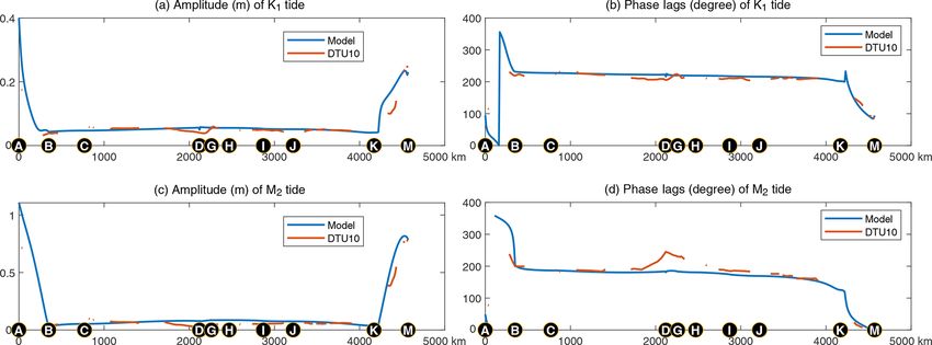
584 D. Wu et al.: Study of the tidal dynamics of the Korea Strait
Table 1. Parameters used in the model. the parameters of 3 pairs of Kelvin waves and 125 pairs of
Poincaré modes can be obtained. Along the open boundary
Parameter Area1 Area2 Area3 Area4 of the KS, the open-boundary condition Eq. (8) is employed,
Wj (km) 230 700 350 140 with the value of ζ̂ equal to the observed harmonic constants
Lj (km) 350 950 400 400 from the global tide model DTU10 (Cheng and Anderson,
wj,1 (km) 250 200 550 760 2011). Along the cross sections connecting Area1 with Area2
fj (10−5 s−1 ) 8.28 9.24 10.10 10.65 and Area2 with Area3, the matching conditions Eq. (9) are
hj (m) 99 2039 1783 90 applied. Along the solid cross sections, condition Eq. (6) is
Nj 22 69 34 13 used.
3.2 Model results and validation
corresponding Kelvin wavelengths, the inequality Re(βj2 −
αj2 ) < π/Wj as stated in the Sect. 2.2 is satisfied (see also The obtained analytical solutions of the K1 and M2 tides us-
Godin, 1965; Fang and Wang, 1966; Wu et al., 2018), Thus ing the extended Taylor method are shown in Fig. 5a and
the Poincaré modes can only exist in a bound form. b, respectively. The maximum amplitude of the K1 tide is
In addition to the parameters listed in Table 1, we need to 0.34 m, which appears at the southwest corner of the KS.
estimate the parameters µM2 and µK1 as defined by Eq. (4). The amplitude decreases from southwest to northeast, and a
Since M2 has the largest tidal current in the KS (Teague et al., counter-clockwise tidal wave system occurs in the northeast
2001), and we assume that the tidal currents are rectilinear, part of the KS, with amplitudes less than 0.05 m near the am-
the linearized frictional coefficient for M2 is approximately phidromic point. A co-tidal line with a phase lag of 210◦ runs
equal to the following, after Pingree and Griffiths (1981), from the amphidromic point in the KS into the southwest JS.
Fang (1987) and Inoue and Garrett (2007), The maximum amplitude of the M2 tide is 1.02 m, which
appears at the westernmost corner of the KS. The amplitude
CD 8 3X 2 decreases gradually from southwest to northeast along the
γM2 ≈ UM2 1 +
i=2, 3,... i
, (26) direction of the strait, and the amphidromic point occurs at
h 3π 4
the junction of the KS and JS. The amplitudes near the am-
where CD is the drag coefficient and UM2 is the tidal cur- phidromic point are lower than 0.1 m, and the phase lags in
rent amplitude of M2 , i = Ui /UM2 , with Ui representing the most parts of the JS vary from 150 to 210◦ . A degenerated
tidal current amplitude of the constituent i (here, we desig- amphidromic point appears near the entrance of the Tartar
nate i = 1 for M2 and i = 2, 3, . . . for any constituents other Strait. The comparison with the tidal charts based on data
than M2 ). According to Fang (1987) and Inoue and Gar- from DTU10 (Fig. 5c, d) shows that the model-produced tidal
rett (2007), the linearized frictional coefficient for the non- systems agree fairly well with the observations.
dominant constituent i is approximately equal to the follow- To quantitatively validate the model results, we first extract
ing: the data along the solid boundary of the model for compari-
son as shown in Fig. 6. For the K1 tide, the model-produced
CD 4 2
1X amplitudes and phase lags along the boundary in the JS both
γi ≈ UM2 1 + i + 2
k = 2, 3, . . . k . (27)
agree well with the observed data, although small differences
h π 8 4
k 6= i occur at the northern corner of the JS. For the M2 tide, the
greatest phase-lag errors are approximately 64◦ near the en-
Inserting Eqs. (26) and (27) into Eq. (4), we can obtain the trance of the Tartar Strait due to the existence of a degener-
parameter µ. Teague et al. (2001) provided tidal current har- ated amphidromic point near this area (Fig. 2b).
monic constants at 10 mooring stations along two cross sec- For further validation, we select 16 tide gauge stations
tions in the KS. The averaged values of the major semi- where harmonic constants are available from the Interna-
axes of the tidal current ellipses at these stations are 0.154, tional Hydrographic Bureau (1930). The station locations are
0.119, 0.101 and 0.062 m s−1 for M2 , K1 , O1 and S2 , respec- shown in Fig. 4. The result of the comparison is given in Ta-
tively. Here, we use these values and CD ≈ 0.0026 to esti- ble 2, which also shows that the model results are consistent
mate the parameters in Eqs. (26) and (27). Then, after insert- with the data obtained from gauge observations: the RMS
ing these values into Eq. (4), we obtain rough estimates of (root mean square) differences of amplitudes of K1 and M2
µM2 and µK1 for the KS (Area1), which are approximately are 0.014 and 0.032 m, respectively; and those of the phase
0.05 and 0.09, respectively. Since the JS is much deeper and lags are 7.0 and 5.2◦ , respectively.
has much weaker tidal currents than the KS, we simply let Although the theoretical model greatly simplifies the to-
µK1 = µM2 = 0 for both Area2 and Area3. pography and boundary, the amplitude and phase-lag differ-
For the collocation approach, we take 10 km as the spacing ences of these two tidal constituents are very small in the
between collocation points. Thus in this model, a total of 198 KS and its surroundings, and the basic characteristics of the
collocation points are used to establish 256 equations, and tidal patterns are well retained (Fig. 5). These findings show
Ocean Sci., 17, 579–591, 2021 https://doi.org/10.5194/os-17-579-2021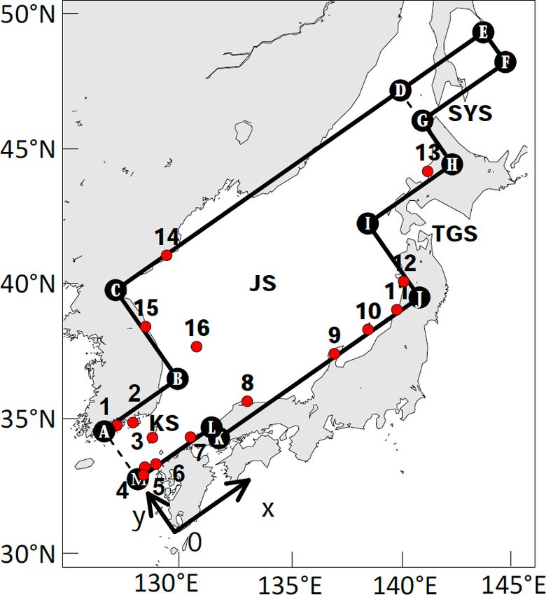
D. Wu et al.: Study of the tidal dynamics of the Korea Strait 585
Figure 5. Comparison of tidal system charts. (a) K1 and (b) M2 tides from the present theoretical model and (c) K1 and (d) M2 tides from
DTU10 (Cheng and Andersen, 2011).
Figure 6. Comparison of model results (blue) and observations based on DTU10 (orange) along the coasts. (a) K1 amplitudes, (b) K1 phase
lags, (c) M2 amplitudes, and (d) M2 phase lags. The locations of the points A, B, C, D, G, H, I, J K, L and M are shown in Fig. 4.
that the simplification of the model is reasonable and the ex- 3.3 Tidal waves in the Korea Strait
tended Taylor method is appropriate for modelling the tides
in the KS–JS basin. Therefore, it is meaningful to use the
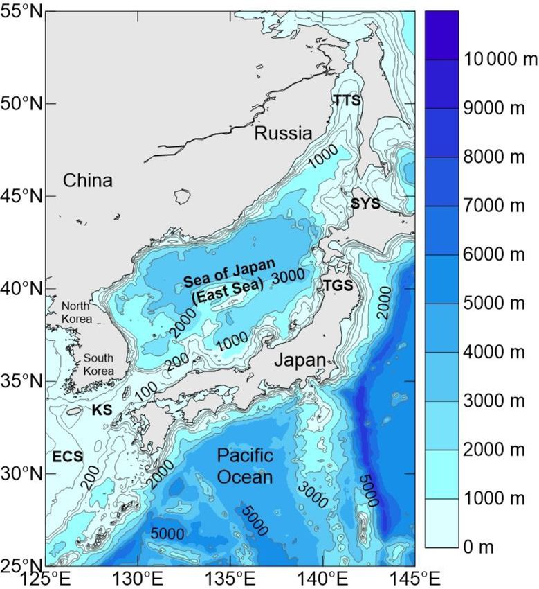
model results for theoretical analysis. To reveal the relative importance of the Kelvin waves versus
Poincaré modes in the modelled Korea Strait, the superpo-
sition of Kelvin waves and that of the Poincaré modes are
given in Fig. 7a–b for K1 and in Fig. 8a–b for M2 .
For the K1 tide in the KS, the superposition of the incident
(northeastward) and the reflected (southwestward) Kelvin
https://doi.org/10.5194/os-17-579-2021 Ocean Sci., 17, 579–591, 2021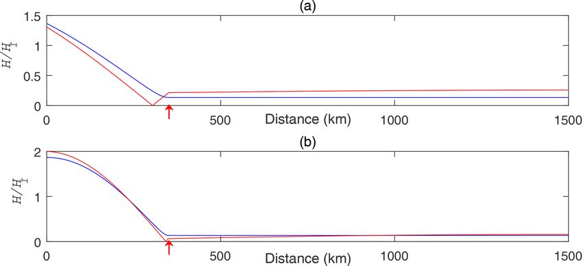
586                                                                    D. Wu et al.: Study of the tidal dynamics of the Korea Strait

Table 2. Comparison between harmonic constants from the observations and models at coastal tide gauge stations.

                No.    Station name                                 K1                                     M2
                                                   Amplitude (m)         Phase lag (◦ )     Amplitude (m)       Phase lag (◦ )
                                                   Obs.    Model         Obs.     Model     Obs.     Model      Obs.     Model
                1      Reisui Ko                   0.21         0.20      50           39   1.02        0.93    357           10
                2      Toei Ko                     0.16         0.12      46           39   0.80        0.76    355            2
                3      Takesiki Ko, Aso Wan        0.12         0.11      83           87   0.66        0.66      1            6
                4      Aokata                      0.23         0.23      90           85   0.80        0.81    356          358
                5      Konoura, Uku Sima           0.20         0.22      92           88   0.78        0.79    354            2
                6      Usuka Wan, Hirado Sima      0.19         0.21     102           97   0.74        0.78      2            8
                7      Kottoi                      0.12         0.13     174          155   0.32        0.34     31           33
                8      Sitirui                     0.04         0.04     206          211   0.06        0.04    152          148
                9      Nakai Iri,Hoku Wan          0.06         0.05     215          214   0.07        0.07    172          164
                10     Ryotu Ko, Sado              0.05         0.05     211          215   0.05        0.07    181          167
                11     Kamo Ko                     0.06         0.05     211          216   0.07        0.07    174          169
                12     Akita                       0.06         0.05     220          216   0.05        0.07    174          170
                13     Hamamasu                    0.05         0.06     211          219   0.05        0.09    185          180
                14     Zyosin Ko                   0.06         0.05     227          227   0.08        0.06    187          185
                15     Sokcho                      0.04         0.05     236          228   0.07        0.05    189          188
                16     Uturyo To                   0.04         0.04     222          226   0.04        0.04    194          180
                       RMS difference                   0.014                   7.0             0.032                  5.2

waves appears as a counter-clockwise amphidromic system,                  and their amplitudes quickly approach zero away from these
with the amphidromic point located near the middle of the                 cross sections. In fact, these properties of the Poincaré wave
strait, but closer to the southeast coast of Korea (Fig. 7a). The         are inherent in any narrow strait. Therefore, in the following,
highest amplitude of the superposed Kelvin waves is 0.3 m,                we will focus on Kelvin waves and analyse the characteris-
and the mean difference from the observations is less than                tics of the incident (northeastward) and reflected (southwest-
0.03 m. The superposition of all Poincaré modes has ampli-                ward) Kelvin waves.
tudes of approximately 0.1 m near the cross sections on both                 The incident and reflected K1 Kelvin waves are shown in
left and right sides, and a counter-clockwise amphidromic                 Fig. 7c and d, respectively. The area-mean amplitude of the
point exists nearly at the centre of the strait (Fig. 7b). Since          incident Kelvin wave in the KS is 0.248 m, and that of the re-
the amplitudes of the superposed Poincaré modes are signifi-              flected Kelvin wave is 0.190 m, which is 77 % of the incident
cantly smaller than those of the superposed Kelvin waves, the             Kelvin wave. On the connecting cross section, the section-
latter can basically represent the total tidal pattern, including         mean amplitude of the incident Kelvin wave is 0.243 m, and
the counter-clockwise amphidromic system.                                 the section-mean phase lag is 151.6◦ . The section-mean am-
   For the M2 tide, the highest amplitude of the superposition            plitude of the reflected Kelvin wave is 0.194 m, which is 80 %
of two Kelvin waves is approximately 0.95 m, which appears                of the incident Kelvin wave. The section-mean phase lag
at the southwest corner of the strait (Fig. 8a). The amplitude            is 295.8◦ , indicating that the phase lag increases by 144.2◦
decreases from southwest to northeast along the strait, and               when the wave is reflected. The amphidromic point of the
the amphidromic point appears near the cross section con-                 superposed Kelvin wave is 137 km away from the step and
necting to the JS, where a topographic step exists. The max-              close to the northwest shore of the KS.
imum deviation of the amplitudes of the superposed Kelvin                    The incident and reflected M2 Kelvin waves are shown in
waves from the observations is 0.06 m, and the structure of               Fig. 8c and d, respectively. The area-mean amplitude of the
the superposed Kelvin waves is consistent with the observa-               incident Kelvin wave in the KS is 0.471 m, and that of the re-
tion. The amplitudes of the superposed Poincaré modes are                 flected Kelvin wave is 0.439 m, which is 93 % of the incident
generally less than 0.2 m on both left and right sides of the             Kelvin wave. This ratio is larger than the K1 tide because
KS, and they decay rapidly towards the middle of the strait,              the bottom friction of M2 is smaller and less energy is lost in
thus forming a counter-clockwise amphidromic system struc-                the propagation process. On the connecting cross section, the
ture (Fig. 8b). Therefore, the M2 tide in the KS is also mainly           mean amplitude of the incident Kelvin wave is 0.462 m, and
controlled by Kelvin waves.                                               the phase lag is 97.9◦ . The mean amplitude of the reflected
   The above results show that the Poincaré modes only ex-                Kelvin wave is 0.447 m, which is 97 % of the incident Kelvin
ist along the open boundary and the connecting cross section              wave, and the phase lag is approximately 266.4◦ , with a

Ocean Sci., 17, 579–591, 2021                                                                      https://doi.org/10.5194/os-17-579-2021
D. Wu et al.: Study of the tidal dynamics of the Korea Strait 587
phase-lag increase of 168.5◦ , which is closer to 180◦ as com- where κR is called the reflection coefficient and is equal to
pared to the corresponding value of the K1 tide. Accordingly, the following:
the M2 amphidromic point of the superposed Kelvin wave
shifts to approximately 21 km away from the step. A com- 1−ρ
κR = . (32)
parison between Figs. 7a and 8a shows that the amphidromic 1+ρ
point of K1 is located west of that of M2 . This result repro- √ √
duces well the observed phenomenon as seen from Fig. 2. If ρ > 1, namely, if h2 W2 > h1 W1 , then κR < 0, Eq. (32)
The above results indicate that the relation of the ampli- can be rewritten in the form
tudes and phase lags of the reflected Kelvin wave with the
incident wave plays a decisive role in the tidal system in the ρ −1
κR = exp(−iπ ). (33)
KS, especially in the formation of amphidromic points, for ρ +1
both the K1 and M2 tides.
The above equation indicates that at the connecting point, the
reflected wave changes its phase lag by 180◦ . Therefore, the
4 Discussion on the formation mechanism of superposition of incident and reflected waves in Area1 has
amphidromic points the minimum amplitude at the connecting point. This theory
explains how the reflected wave can be generated by abrupt
To explore the tidal dynamics of the KS–JS basin, espe- increases in water depth and basin width, and why the re-
cially the formation mechanism of amphidromic points, we flected wave there has a phase lag opposite to the incident
consider the simplest case: a one-dimensional tidal model wave.
in channels. In the one-dimensional case, the amphidromic The complete solution for this case is as follows (see also
point is equivalent to the wave node. As previously men- Dean and Dalrymple, 1984):
tioned, an important feature of the topography of the KS–
JS basin is that there is a steep continental slope between
ρ−1
the KS and JS, and to the northeast of this slope, the JS is
ζ (x) = HI exp{−i [k1 (x − l1 ) + θ1 ]} + ρ+1
much deeper and wider than the KS. Thus, the channel is
exp{−i [−k1 (x − l1 ) + 2χ1 + θ1 + π ]} ,
idealized to contain two areas, with the first one (Area1) hav- (34)
ing uniform depth h1 and uniform width W1 and the second
l1
x
l2
one (Area2) having uniform depth h2 and uniform width W2 .
2
ζ (x) = 1+ρ HI exp{−i [k2 (x − l2 ) + χ1 + θ1 ]},
Therefore, the idealized channel contains abrupt changes in
l2
x
depth and width at the connection of these two areas. An in-
cident wave enters the first area and propagates toward the
where θ1 represents the phase lag of the incident wave at
second area passing over the topographic step. For simplic-
the opening of Area1; kj = σ/cj is the wave number, with
ity, we neglect friction. p
cj = ghj representing the wave speed in Areaj , j = 1,
If the second area is semi-infinitely long, allowing for the
2; and χ1 = k1 L1 . This solution for the K1 and M2 con-
wave radiating out from the second area freely, then a part
stituents for h1 = 99 m, L1 = 350 km, W1 = 230 km, h2 =
of the wave is reflected at the connecting point and another
2039 m and W2 = 700 km is plotted with the blue curves in
part is transmitted into the second area. The amplitude of the
Fig. 9.
transmitted wave is (see for example Dean and Dalrymple,
However, Sect. 3.3 shows that the phase-lag changes of the
1984)
reflected waves relative to the incident waves are not exactly
HT = κ T HI , (28) equal to 180◦ but rather are smaller than 180◦ , and the dis-
crepancy increases with the decreasing angular frequency. To
where HI is the amplitude of the incident wave and κT is
explain this discrepancy, we improve the above theory by in-
called the transmission coefficient, which is equal to
troducing the reflected wave in the second area. In fact, the JS
2 is represented with a semi-closed area in the two-dimensional
κT = , (29)
1+ρ model (Sect. 3.1), namely, all boundaries except those con-
where nected to KS are solid ones (Fig. 4). Therefore, in the fol-
√ lowing one-dimensional model, the second area is closed at
c2 W2 h2 W2 its right end so that the reflection will occur at this end. In
ρ= =√ , (30)
c1 W1 h1 W1 this case, the solution becomes more complicated and is de-
p pendent on the length of the second area L2 . The reflection
with cj = ghj representing the wave pspeed in the j th area; coefficient κR now has the following form (see Supplement
j = 1, 2. cj is in fact proportional to hj . The amplitude of
for derivation):
the reflected wave HR is
HR = κ R HI , (31) κR = exp(−i2δ), (35)
https://doi.org/10.5194/os-17-579-2021 Ocean Sci., 17, 579–591, 2021588 D. Wu et al.: Study of the tidal dynamics of the Korea Strait Figure 7. Decomposed charts for the model-produced K1 tide in the Korea Strait: (a) contribution of Kelvin waves, (b) contribution of Poincaré modes, (c) northeastward (incident) Kelvin wave and (d) southwestward (reflected) Kelvin wave. Figure 8. Same as in Fig. 7 but for M2 . Ocean Sci., 17, 579–591, 2021 https://doi.org/10.5194/os-17-579-2021
D. Wu et al.: Study of the tidal dynamics of the Korea Strait 589
in which δ is determined by the following equations:
1+cos 2χ2
cos δ = 2
,
2 1/2
(1+cos 2χ2 ) +(ρ sin 2χ2 )
ρ sin 2χ2 (36)
sin δ = 1/2 ,
(1+cos 2χ2 )2 +(ρ sin 2χ2 )2
where χ2 = k2 L2 . Equation (36) indicates that the length,
width and depth of Area2 are also important in determin-
ing the phase-lag increase of the reflected wave relative to
the incident wave in Area1. Comparison of Eq. (35) with
Eq. (33) indicates that the phase-lag increase is now 2δ in-
Figure 9. Amplitude distribution along the channel. (a) K1
stead of π . The difference 1 = π −2δ characterizes the influ-
and (b) M2 . Blue/red curves are solutions for semi-infinite/finite
ence of Area2 upon the phase-lag increase at the connection Area2. The red arrow indicates the position of the connecting point
of two areas. To show the influence of the length, width and between the Korea Strait and the Japan Sea. Amplitudes are given
depth of Area2 on the value of 1, we first retain the width as ratios to the incident wave in Area1.
and depth unchanged and increase the length by 10 %; it is
shown that the value of 1 for K1 is reduced by 15 % (re-
duced to 10.44◦ from 12.27◦ ) and that the value of 1 for M2
is reduced by 37 % (reduced to 2.37◦ from 3.78◦ ). Next we
retain the length and depth unchanged and increase the width
by 10 %; it is shown that the value of 1 for K1 is reduced by
9 % (reduced to 11.16◦ from 12.27◦ ) and that the value of
1 for M2 is reduced by 9 % (reduced to 3.44◦ from 3.78◦ ).
Then we retain the length and width unchanged and increase
the depth by 10 %; it is shown that the value of 1 for K1 in- Figure 10. Phase-lag increase of the reflected wave relative to the
creases by 1 % (increases to 12.42◦ from 12.27◦ ) and that the incident wave as a function of the angular velocity at the connecting
value of 1 for M2 increases by 9 % (increases to 4.12◦ from point. See the text for details.
3.78◦ ).
The complete solution for this case is as follows:
This result is natural because friction is not considered and
no dissipation is present during wave propagation. Equa-
ζ (x) = H I exp{−i [k1 (x − l1 ) + θ1 ]}
tion (35) also indicates that the phase lag of the reflected
wave at the connecting point is greater than that of the in-
+ exp{−i [−k1 (x − l1 ) + 2χ1 + θ1 + 2δ]} ,
cident wave at the same point by 2δ. Since the node of the
l1
x
l2 superposition of the incident and reflected waves appears at
(37) the place where the phase lags of these two waves are oppo-
ζ (x) = H I exp{−i [k 2 (x − l 2 ) + (χ1 + φ + θ1 )]} site, the first node should appear at 1x away from the con-
necting point with
+ exp{−i [−k2 (x − l2 ) + (2χ2 + χ1 + φ + θ1 )]} ,
1x = (π − 2δ)/ (2k1 ) . (39)
l2
x
l3
The above relationship can also be obtained from the first
where ε = 2E −1 . E and φ are determined by the following equation of Eq. (37). The dependence of 2δ on σ for the
relations: case h1 = 99 m, L1 = 350 km, W1 = 230 km, h2 = 2039 m,
E cos φ = (ρ + 1) − (ρ − 1) cos 2χ2 , L2 = 1150 km and W2 = 700 km is plotted in Fig. 10. This
(38) figure shows that 2δ = 0 when σ = 0 and 2δ increases with
E cos φ = (ρ − 1) sin 2χ2 .
increasing σ , although it is always less than 180◦ . In par-
The first terms on the right-hand side of the two equations ticular, 2δ = 167.7◦ when σ = σK1 and 2δ = 176.2◦ when
in Eq. (37) represent the waves propagating in the posi- σ = σM2 . Based on this theory, the M2 and K1 amphidromic
tive x direction, and the second terms are those propagat- points should be located at 7.4 and 45.9 km away from
ing in the negative x direction. This solution for the K1 and the connecting point, respectively. Compared with the two-
M2 constituents for the case h1 = 99 m, L1 = 350 km, W1 = dimensional model results given in Sect. 3.3, this theory
230 km, h2 = 2039 m, L2 = 1150 km and W2 = 700 km is roughly explains one-third of the changes. The remaining
plotted with the red curves in Fig. 9. two-thirds of the changes may be due to the effect of the
Equation (35) indicates that the amplitude of the reflected Coriolis force. The solution of phase-lag changes at the cross
wave in the first area is equal to that of the incident wave. section in the two-dimensional rotating basin involves in-
https://doi.org/10.5194/os-17-579-2021 Ocean Sci., 17, 579–591, 2021590 D. Wu et al.: Study of the tidal dynamics of the Korea Strait
teractions among three Kelvin waves (an incident and a re- Data availability. The ETOPO1 data
flected Kelvin wave in Area1 and a transmitted Kelvin wave (https://doi.org/10.7289/V5C8276M, Amante and Eakins,
in Area2) and two families of Poincaré modes at the connect- 2009) are from the National Geophysical Center, USA
ing cross section (one family in each area). Taylor (1922), (https://www.ngdc.noaa.gov/mgg/global/, last access:
Fang and Wang (1966) and Thiebaux (1988) have studied the 14 June 2016). The DTU10 tidal data are from DTU Space,
Danish National Space Center, Technical University of Denmark
Kelvin-wave reflection at the closed cross section of semi-
(ftp://ftp.space.dtu.dk/pub/DTU10/DTU10_TIDEMODEL, last
infinite rotating two-dimensional channels. In their studies, access: 3 February 2012, Cheng and Andersen, 2011).
only two Kelvin waves and one family of Poincaré modes
were involved. In comparison to their studies, the present
problem is much more complicated. Because of the com- Supplement. The supplement related to this article is available on-
plexity of the problem, we will presently leave it for a future line at: https://doi.org/10.5194/os-17-579-2021-supplement.
study.
Author contributions. GF conceived the study scope and the basic
5 Summary
dynamics. DW performed calculation and prepared the draft. ZW
and XC checked model results.
In this paper, we establish a theoretical model for the KS–JS
basin using the extended Taylor method. The model idealizes
the study region as three connected flat rectangular areas, in-
Competing interests. The authors declare that they have no conflict
corporates the effects of the Coriolis force and bottom fric- of interest.
tion in the governing equations, and is forced by observed
tides at the opening of the KS. The analytical solutions of the
K1 and M2 tidal waves are obtained using Defant’s colloca- Acknowledgements. We sincerely thank Joanne Williams for han-
tion approach. dling our paper and thank David Webb and Kyung Tae Jung for
The theoretical model results are consistent with the satel- their careful reading of our paper and constructive comments and
lite altimeter and tidal gauge observations, which indicates suggestions which were of great help in improving our work.
that the model is suitable and correct. The model reproduces
well the K1 and M2 tidal systems in the KS. In particular, the
model-produced locations of the K1 and M2 amphidromic Financial support. This research has been supported by the Na-
points are consistent with the observed ones. tional Natural Science Foundation of China (grant nos. 41706031
The model solution provides the following insights into and 41821004).
the tidal dynamics in the KS. (1) The tidal system in each
rectangular area can be decomposed into two oppositely trav-
elling Kelvin waves and two families of Poincaré modes, Review statement. This paper was edited by Joanne Williams and
reviewed by Kyung Tae Jung and David Webb.
with Kelvin waves dominating the tidal system due to the
narrowness of the area. (2) The incident Kelvin wave from
the ECS through the opening of the KS travels toward the
JS and is reflected at the connecting cross section between References
the KS and JS, where abrupt increases from the KS to JS in
water depth and basin width occur. (3) The phase lag of the Amante, C. and Eakins, B. W.: ETOPO1 1 Arc-Minute
reflected wave at the connecting cross section increases by Global Relief Model: Procedures, Data Sources and Analysis,
less than 180◦ relative to that of the incident wave, thus en- https://doi.org/10.7289/V5C8276M, 2009.
abling the formation of the amphidromic points in the KS. Book, J. W., Pistek, P., Perkins, H., Thompson, K. R., Teague,
W. J., Jacobs, G. A., Suk, M. S., Chang, K. I., Lee, J. C.,
(4) The phase-lag increase of the reflected wave relative to
and Choi, B. H.: Data Assimilation modeling of the barotropic
the incident wave is dependent on the angular frequency of tides in the Korea/Tsushima Strait, J. Oceanogr., 60, 977–993,
the wave and becomes smaller as the angular frequency de- https://doi.org/10.1007/s10872-005-0006-6, 2004.
creases. This feature explains why the K1 amphidromic point Carbajal, N.: Two applications of Taylor’s problem solution for fi-
is located farther away from the connecting cross section in nite rectangular semi-enclosed basins, Cont. Shelf Res., 17, 803–
comparison to the M2 amphidromic point. (5) The length, 808, https://doi.org/10.1016/S0278-4343(96)00058-1, 1997.
width and depth of the JS is also important in determining Cheng, Y. C. and Andersen, O. B.: Multimission empir-
the phase-lag increase of the reflected Kelvin wave in the ical ocean tide modeling for shallow waters and po-
KS. lar seas, J. Geophys. Res.-Ocean., 116, 1130–1146,
https://doi.org/10.1029/2011JC007172, 2011.
Choi, B. H., Kim, D. H., and Fang, Y.: Tides in the East Asian Seas
from a fine-resolution global ocean tidal model, Mar. Technol.
Soc. J., 33, 36–44, https://doi.org/10.4031/MTSJ.33.1.5, 1999.
Ocean Sci., 17, 579–591, 2021 https://doi.org/10.5194/os-17-579-2021D. Wu et al.: Study of the tidal dynamics of the Korea Strait 591 Dean, G. and Dalrymple, R.: Water wave mechanics for engineers Odamaki, M.: Tides and tidal currents in the Tusima Strait, and scientists, World Scientific, Singapore, 353 pp., 1984. J. Oceanogr., 45, 65–82, https://doi.org/10.1007/BF02108795, Defant, A.: Physical oceanography, Vol. II, Pergamon Press, New 1989a. York, 598 pp., 1961. Odamaki, M.: Co-oscillating and independent tides of Fang, G.: Nonlinear effects of tidal friction, Acta Oceanol. Sin., 6, the Japan Sea, J. Oceanogr. Soc. Jpn, 45, 217–232, 105–122, 1987. https://doi.org/10.1007/BF02123465, 1989b. Fang, G. and Wang, J.: Tides and tidal streams in gulfs, Oceanol. Ogura, S.: The Tides in the Seas Adjacent to Japan. Bulletin of Limnol. Sin., 8, 60–77, 1966 (in Chinese with English abstract). the Hydrographic Department, Imperial Japanese Navy, Tokyo, Fang, G. and Yang, J.: Modeling and prediction of tidal cur- 7, 189 pp., 1933. rents in the Korea Strait, Prog. Oceanogr., 21, 307–318, Pingree, R. D. and Griffiths, D. K.: The N2 tide and semidiurnal am- https://doi.org/10.1016/0079-6611(88)90010-9, 1988. phidromes around the British Isles, J. Mar. Biol. Assoc. UK, 61, Fang, Z., Ye, A., and Fang, G.: Solutions of tidal motions in a semi- 617–625, https://doi.org/10.1017/S0025315400048086, 1981. closed rectangular gulf with open boundary condition specified, Rienecker, M. M. and Teubner, M. D.: A note on frictional effects Tidal Hydrodynamics, edited by: Parker, B. B., John Wiley & in Taylor’s problem, J. Mar. Res., 38, 183–191, 1980. Sons. Inc., New York, 153–168, 1991. Roos, P. C. and Schuttelaars, H. M.: Influence of topography on tide Godin, G.: Some remarks on the tidal motion in a narrow rect- propagation and amplification in semi-enclosed basins, Ocean angular sea of constant depth, Deep-Sea Res., 12, 461–468, Dynam., 61, 21–38, https://doi.org/10.1007/s10236-010-0340-0, https://doi.org/10.1016/0011-7471(65)90400-6, 1965. 2011. Hendershott, M. C. and Speranza, A.: Co-oscillating tides in long, Roos, P. C., Velema, J. J., Hulscher, S. J. M. H., and Stolk, A.: narrow bays; the Taylor problem revisited, Deep-Sea Res., 18, An idealized model of tidal dynamics in the North Sea: Reso- 959–980, https://doi.org/10.1016/0011-7471(71)90002-7, 1971. nance properties and response to large-scale changes, Ocean Dy- International Hydrographic Bureau: Tides, Harmonic Constants, In- nam., 61, 2019–2035, https://doi.org/10.1007/s10236-011-0456- ternational Hydrographic Bureau, Special Publication No. 26 and x, 2011. addenda, data set, 1930. Takikawa, T., Yoon, J. H., and Cho, K. D.: Tidal Inoue, R. and Garrett, C.: Fourier Representation of Currents in the Tsushima Straits estimated from Quadratic Friction, J. Phys. Oceanogr., 37, 593–610, ADCP data by ferryboat, J. Oceanogr., 59, 37–47, https://doi.org/10.1175/JPO2999.1, 2007. https://doi.org/10.1023/A:1022864306103, 2003. Jung, K. T., Park, C. W., Oh, I. S., and So, J. K.: An ana- Taylor, G. I.: Tidal oscillations in gulfs and rectangu- lytical model with three sub-regions for M2 tide in the Yel- lar basins, Proc. London Math. Soc. Ser., 2, 148–181, low Sea and the East China Sea, Ocean Sci. J., 40, 191–200, https://doi.org/10.1112/plms/s2-20.1.148, 1922. https://doi.org/10.1007/BF03023518, 2005. Teague, W. J., Perkins, H. T., Jacobs, G. A., and Book, J. W.: Kang, S. K., Lee, S. R., and Yum, K. D.: Tidal computation of the Tide observation in the Korea-Tsushima Strait, Cont. Shelf Res., East China Sea, the Yellow Sea and the East Sea, Oceanography 21, 545–561, https://doi.org/10.1016/S0278-4343(00)00110-2, of Asian Marginal Seas, edited by: Takano, K., Elsevier, Ams- 2001. terdam, 25–48, https://doi.org/10.1016/S0422-9894(08)70084-9, Thiebaux, M. L.: Low-frequency Kelvin wave reflection coefficient, 1991. J. Phys. Oceanogr., 18, 367–372, https://doi.org/10.1175/1520- Matsumoto, K., Takanezawa, T., and Ooe, M.: Ocean tide mod- 0485(1988)0182.0.CO;2, 1988. els developed by assimilating TOPEX/POSEIDON altime- Webb, D. J.: A model of continental-shelf resonances, Deep-Sea ter data into hydrodynamical model: a global model and Res., 23, 1–15, https://doi.org/10.1016/0011-7471(76)90804-4, a regional model around Japan, J. Oceanogr., 56, 567–581, 1976. https://doi.org/10.1023/A:1011157212596, 2000. Wu, D., Fang, G., Cui, X., and Teng, F.: An analytical study of Morimoto, A., Yanagi, T., and Kaneko, A.: Tidal correction of M2 tidal waves in the Taiwan Strait using an extended Taylor altimetric data in the Japan Sea, J. Oceanogr., 56, 31–41, method, Ocean Sci., 14, 117–126, https://doi.org/10.5194/os-14- https://doi.org/10.1023/A:1011158423557, 2000. 117-2018, 2018. https://doi.org/10.5194/os-17-579-2021 Ocean Sci., 17, 579–591, 2021
You can also read