Forecasting daily meteorological time series using ARIMA and regression models
←
→
Page content transcription
If your browser does not render page correctly, please read the page content below
Int. Agrophys., 2018, 32, 253-264
doi: 10.1515/intag-2017-0007

  Forecasting daily meteorological time series using ARIMA and regression models**
                 Małgorzata Murat1, Iwona Malinowska1, Magdalena Gos2, and Jaromir Krzyszczak2*
             1
              Department of Mathematics, Lublin University of Technology, Nadbystrzycka 38a, 20-618 Lublin, Poland
                 2
                   Institute of Agrophysics, Polish Academy of Sciences, Doświadczalna 4, 20-290 Lublin, Poland

                                       Received September 20, 2017; accepted January 31, 2018

    Ab s t r a c t. The daily air temperature and precipitation time   these models (Hoffmann et al., 2017; Krzyszczak et al.,
series recorded between January 1, 1980 and December 31, 2010          2017b; Walczak et al., 1997). When taking into account
in four European sites (Jokioinen, Dikopshof, Lleida and Lublin)       the global warming effects on the processes occurring
from different climatic zones were modeled and forecasted. In our      in the soil-plant-atmosphere system, the shifts in future
forecasting we used the methods of the Box-Jenkins and Holt-           weather patterns and the increase in frequency and mag-
Winters seasonal auto regressive integrated moving-average, the
                                                                       nitude of extreme events should be known (Lobell et al.,
autoregressive integrated moving-average with external regres-
sors in the form of Fourier terms and the time series regression,
                                                                       2012; Semenov and Shewry, 2011; Sillmann and Roeckner,
including trend and seasonality components methodology with R          2008). Increasing temperature and limited precipitation,
software. It was demonstrated that obtained models are able to         which are responsible for drought incidence as a result of
capture the dynamics of the time series data and to produce sen-       global warming, are posing serious threats to food security
sible forecasts.                                                       (Lobell et al., 2013). The forecasting of these two quantities
    Ke y w o r d s: regression models, forecast, time series, meteo-   using statistical methods is, therefore, of great importance.
rological quantities                                                       Many time series forecasting methods are based on the
                                                                       analysis of historical data. They assume that past patterns
                        INTRODUCTION                                   in the data can be used to forecast future events. In recent
    The prediction of the future courses of meteorological             years, one of the most popular ways of time series model-
quantities on the basis of historical time series is impor-            ling is autoregressive integrated moving-average (ARIMA)
tant for agrophysical modelling (Lamorski et al., 2013;                modelling. Its main aim is to carefully and rigorously study
Baranowski et al., 2015; Murat et al., 2016; Krzyszczak                the past observations of a time series to develop an appro-
et al., 2017a). All the crop production models are highly              priate model which can predict future values for the series.
sensitive to climatic and environmental variations (Fronzek            It has three control constants i.e. irregular, trend and sea-
et al., 2018; Pirttioja et al., 2015; Porter and Semenov,              sonal influence, which can control and manage influence
2005; Ruiz-Ramos et al., 2018) and the temporal and space              of time segmentation through the specific time duration. In
scaling properties of the weather time series should be con-           literature, ARIMA models have been widely used for vari-
sidered when applying weather time series as the inputs to             ous applications such as medicine, business, economics,
                                                                       finance and engineering. Moreover, ARIMA models have
                                                                       become, in last decades, a major tool in numerous mete-
*Corresponding author e-mail: jkrzyszczak@ipan.lublin.pl
**This work was co-funded by the Polish National Centre for            orological applications to understand the phenomena of air
Research and Development as part of the GyroScan project con-          temperature and precipitation. El-Mallah and Elsharkawy
tract No. BIOSTRATEG2/298782/11/NCBR/2016. We acknowl-                 (2016) showed that the linear ARIMA model and the
edge the data providers in the European Climate Assessment &           quadratic ARIMA model had the best overall performance
Dataset project (ECA&D) − for Lleida, the State Meteorological         in making short-term predictions of annual absolute
Agency. Data and metadata are available at www.ecad.eu. This
work was also part of the FACCE JPI Knowledge Hub ‘Modelling
European Agriculture with Climate Change for Food Safety’ pro-           © 2018 Institute of Agrophysics, Polish Academy of Sciences
ject (MACSUR) contract FACCE JPI/06/2012).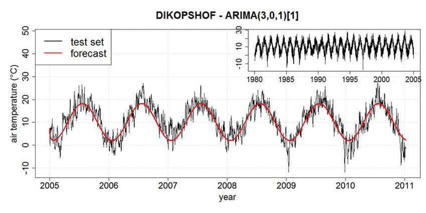
254                                                         M. MURAT et al.

Ta b l e 1. The basic characteristics of the sites and their agro-climatic conditions

                                                                              Site/Country
 Parameter                         Dikopshof                    Jokioinen                      Lleida             Lublin
                                  Germany (DE)                 Finland (FI)                  Spain (ES)         Poland (PL)

 Latitude (°N)                      50°48’29’’                    60°48’                      41°42’             51°14’55’’

 Longitude (°E)                      6°57’7’’                     23°30’                        1°6’             22°33’37’’

 Altitude (m)                           60                         104                          337                 194

 Environmental zone              Atlantic Central                 Boreal                Mediterranean South      Continental

 Köppen-Geiger climate
                                       Cfb                         Dfc                          BSk                 Dfb
 classification

temperature in Libya. Balyani et al. (2014) used ARIMA                 develop predictive models to forecast the daily mean values
model in a 50-year time period (1955-2005) for Shiraz,                 of these quantities up to six years ahead, using the above-
south of Iran. Their modelling of temperature selected                 mentioned methods with external regressors in the form of
ARIMA as the optimal model. Furthermore, Anitha et al.                 Fourier terms.
(2014) used the seasonal autoregressive integrated moving
average (SARIMA) model to forecast the monthly mean of                                            MATERIALS
the maximum surface air temperature of India. Their results                We decided to study four sites from northern, central
showed that there is a trend in the monthly mean of maxi-              and southern Europe in order to represent contrasting cli-
mum surface air temperature in India. Muhammet (2012)                  matic conditions. Jokioinen in Finland was chosen for
also used the ARIMA method to predict the temperature                  northern Europe and Lleida in Spain for southern Europe.
and precipitation in Afyonkarahisar Province, Turkey,                  For central Europe, two sites were chosen: Dikopshof –
until the year 2025, and found an increase in temperature              located in the west of Germany, and Lublin – in the east of
according to the quadratic and linear trend models. Finally,           Poland. The chosen sites represent boreal, Atlantic central,
Khedhiri (2014) studied the statistical properties of histori-         continental and Mediterranean south climates. The prin-
cal temperature data in Canada for the period 1913-2013                cipal characteristics of these sites and their agro-climatic
and determined a seasonal ARIMA model for the series to                conditions are summarised in Table 1.
predict future temperature records.                                        The Jokioinen site has a subarctic climate that has
     Akpanta et al. (2015) adopted the SARIMA modelling                severe winters, no dry season, with cool, short summers
of the frequency approach in analysing monthly rainfall                and strong seasonality (Köppen-Geiger classification: Dfc,
data in Umuahia. Abdul-Azziz et al. (2013) and Afrifa-                 which means continental subarctic climate with the cold-
Yamoah (2016) forecasted monthly rainfall in several                   est month averaging below 0°C; 1 to 3 months averaging
regions in Ghana with the use of the SARIMA models. The                above 10°C and no significant precipitation difference
SARIMA models of the weekly and monthly rainfall time                  between seasons). Lleida has a semi-arid climate with
series of two selected weather stations in Malaysia were               Mediterranean-like precipitation patterns (annual aver-
built by Yusof and Kane (2012) and in India by Dabral and              age of 369 mm), foggy and mild winters and hot and
Murry (2017). The mentioned ARIMA models have a good                   dry summers (Köppen-Geiger classification: BSk, which
post-sample forecasting performance for yearly and month-              means dry cold semi-arid climate). Dikopshof represents
ly agrometeorological time series.                                     a maritime temperate climate (Köppen-Geiger climate clas-
     Another approach in forecasting the meteorological                sification: Cfb, which means temperate oceanic climate with
time series involves fitting regression models (RM) to time            the coldest month averaging above 0°C, all months with
series including trend and seasonality components. The                 average temperatures below 22°C and at least four months
RM models are originally based on linear modelling, but                averaging above 10°C and no significant precipitation dif-
they also allow parameters such as trend and season to be              ference between seasons). There is significant precipitation
added to the data. In our study, the trend parameter will be           throughout the year in the German site. The Lublin site
fitted with polynomial function, and the season parameter              has a warm summer continental climate (Köppen-Geiger
will be estimated with Fourier series.                                 climate classification: Dfb, which means warm-summer
     The aim of this paper is to examine the statistical proper-       humid continental climate with the coldest month averag-
ties of the daily mean air temperature and the precipitation           ing below 0°C, all months with average temperatures below
time series from four different locations in Europe and to             22°C and at least four months averaging above 10°C and no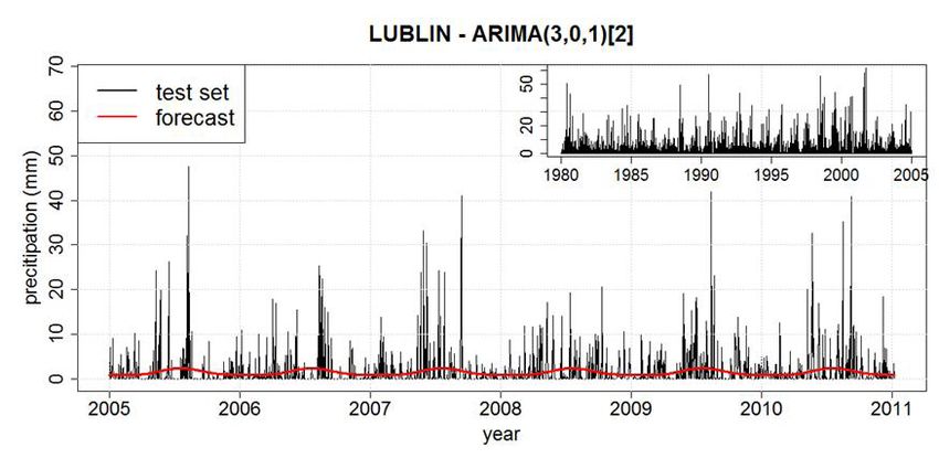
DAILY METEOROLOGICAL TIME SERIES MODELS                                                       255

Ta b l e 2. Descriptive statistics of the whole daily, 31-year meteorological time series – from four stations in Germany (DE), Finland
(FI), Poland (PL) and Spain (ES)

 Meteorological
                Site                     Mean           Min           Max           Std         Median       Skewness      Kurtosis
 variable

                  Dikopshof (DE)          10.2         -16.8          28.9          6.8          10.5          -0.2           2.5

 Air              Jokioinen (FI)           4.6         -33.4          25.0          9.3           4.7          -0.4           2.8
 temperature
 (°C)             Lleida (ES)             15.0          -8.3          33.1          7.6          14.7           0.0           2.1

                  Lublin (PL)              8.7         -22.8          28.3          8.8           9.1          -0.2           2.4

                  Dikopshof (DE)           1.7          0.0           75.4          3.8           0.0           4.5          38.1

 Precipitation    Jokioinen (FI)           1.7          0.0           79.1          3.9           0.1           5.0          49.3
 (mm day-1)       Lleida (ES)              0.9          0.0           83.6          3.8           0.0           7.2          75.7

                  Lublin (PL)              1.5          0.0           61.6          3.9           0.0           5.7          49.7
Mean, min, max, standard deviation (Std) and median have the units corresponding to the units of meteorological variables; skewness
and kurtosis are non-dimensional.
significant precipitation difference between seasons). The           et al., 2008). The ARIMA model was popularised by
weather time series in all sites were measured with stand-           Box and Jenkins (1970) and Box and Tiao (1975). It is
ard equipment, comparable for all stations. In the present           a combination of three mathematical models, using auto-
study, we focus on an air temperature dataset collected on           regressive, integrated, moving-average (ARIMA) models
a daily basis from January 1, 1980 to December 31, 2010              for time series data. An ARIMA (p, d, q) model can account
(11 322 days). The descriptive statistics of the meteorologi-        for temporal dependence in several ways. Firstly, the time
cal time series are presented in Table 2. The highest mean           series is d-differenced to render it stationary. If d = 0, the
and median values of air temperature in the period of 31             observations are modelled directly, and if d = 1, the dif-
years were observed at the Lleida station and the lowest             ferences between consecutive observations are modelled.
at the Jokioinen station. The parameters of skewness and             Secondly, the time dependence of the stationary process
kurtosis of the analysed time series give information about          {Xt} is modelled by including p auto-regressive models.
differences in their statistical distributions. Air temperature      The equation for p is:
is characterised by negative skewness and small kurtosis,
which inform us that this distributions is left-tailed.                                                 φi                          (1)
    A completely different distribution shape can be ob-
served for precipitation, with higher positive skewness and          where: c is the constant, φ is the parameter of the model,
very high kurtosis values for all the stations. This means           xt is the value that observed at t and εt stands for random
that this distribution is strongly right-tailed and has a very       error. Thirdly, q are moving-average terms, in addition to
sharp peak and a fat tail.                                           any time-varying covariates. It takes the observation of pre-
                                                                     vious errors. The equation for q is:
                          METHODS
    A time series is an ordered sequence of values of a va-                                                                         (2)
riable at equally spaced time intervals, i.e. hourly tem-
peratures at a weather station. The main aim of time series          where: θi is the parameter of the model, εt is the error
modelling is to carefully analyse and rigorously process the         term. Finally, by combining these three models, we get
past observations of the time series to develop an appro-            the ARIMA model. Thus, the general form of the ARIMA
priate model which describes the inherent structure of the           models is given by:
series. This makes it possible to explain the data in such
a way as to facilitate prediction, monitoring, or control.                                        φi
There are several approaches to modelling series with                                                                               (3)
a single seasonal pattern. Among these are exponential
smoothing (Winters, 1960), seasonal ARIMA models                     where: Yt is a stationary stochastic process, c is the constant,
(Box and Jenkins, 1970), state-space models (Harvey,                 εt is the error or white noise disturbance term, φi means
1989) and the innovations State Space Models (Hyndman                auto-regression coefficient and θj is the moving average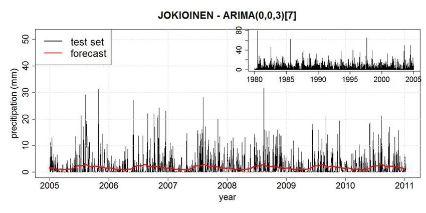
256                                                      M. MURAT et al.

coefficient. For a seasonal time series, these steps can be         respectively, where n is the number of periods of time and
repeated according to the period of the cycle, whatever time        et = yt - ft is the forecast error between the actual value yt
interval. Usually, ARIMA models are described using the             and the forecasted value ft. The MAE is the average over the
backward operator B defined as:                                     verification sample of the absolute values of the differences
                                                                    between the forecast and the corresponding observation.
                 Bk(Xt) = Xt-k t>k; t, k є N,                (4)    Moreover, the RMSE is the square root of the average
where: k is the index denoting how many times backward              squared values of the differences between forecast and the
operator B is applied to time series Xt characterised by time       corresponding observation. These errors have the same
interval t, and N is the total number of time intervals. By         units of measurement and depend on the units in which the
employing the following notation:                                   data are measured. The MASE was proposed by Hyndman
                                                                    and Koehler (2006) for comparing forecast accuracies. The
                                                                    MASE is given by the formula:
                                                             (5)

                                                                                                                              (11)

                                                             (6)    where: Q is a scaling statistic, computed on the training
                                                                    data. For a non-seasonal time series, a useful way to define
the Eq. (1) can be written, respectively, as:                       scaling statistics is to apply the mean absolute difference
                                                                    between the consecutive observations:
                                                             (7)
                                                                                                   n
    The seasonal ARIMA (p, d, q) (P, D, Q)m process noted                                                                     (12)
also as SARIMA (p, d, q) (P, D, Q)m is given by:

                                                             (8)    that is, Q is the MAE for naive forecasts, computed on the
                                                                    training data. The MASE is less than one if it arises from
where: m is the seasonal period, Φ(z) and Θ(z) are polyno-          a better forecast than the average naive forecast computed
mials of orders P and Q, respectively, each containing no           on the training data. Conversely, it is greater than one if the
roots inside the unit circle. If c ≠ 0, there is an implied         forecast is worse than the average naive forecast computed
polynomial of order d + D in the forecast function (Box             on the training data. For a seasonal time series, a scaling
et al., 2008; Brockwell and Davis, 1991). To determine a            statistic can be defined using the seasonal naive forecasts:
proper model for a given time series data, it is necessary to
                                                                                                   n
carry out the Autocorrelation Function (ACF) and Partial
Autocorrelation Function (PACF) analysis, which reflect                                                                       (13)
how the observations in a time series are interrelated.
The plot of ACF helps to determine the order of Moving              where the seasonal naive method accounts for seasonality
Average terms, and the plot of PACF helps to find Auto-             by setting each prediction to be equal to the last observed
Regressive terms.                                                   value of the same season. The MASE is independent of
    The main task in SARIMA forecasting is selecting an             the scale of the data, so it can be used to compare forecasts
appropriate model order; that is, if the values p, q, P, Q, D, d.   for data sets with different scales. When comparing fore-
If d and D are known, we can select the orders p, q, P and          casting methods, the method with the lowest MASE is the
Q via one of the forecast measure error: the mean absolute          preferred one.
error (MAE), the root mean squared error (RMSE) and the                 Sometimes the SARIMA model does not tend to give
mean absolute scaled error (MASE). MAE and RMSE are                 good results for the time series with a period greater than
defined by the formulas:                                            200 years. In such a situation, the simplest approach is a re-
                                                                    gression with ARIMA errors, where the order of the
                                                             (9)    ARIMA model and the number of Fourier terms is selected
                                                                    by minimising the RMSE, MAE or MASE. In such models,
                                                                    external regressors in the form of Fourier terms are added
                                                                    to an ARIMA (p, d, q) model to account for the seasonal
                                                                    behaviour. We can consider ARIMA models with regres-
                                                            (10)    sors as a regression model which includes a correction for
                                                                    autocorrelated errors. Hence, we can add ARIMA terms to
                                                                    the regression model to eliminate the autocorrelation and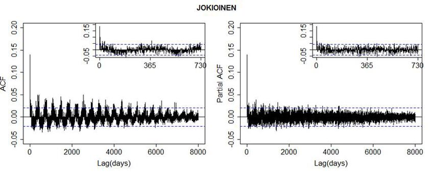
DAILY METEOROLOGICAL TIME SERIES MODELS                                                  257

further reduce the mean squared error. To do this, we re-fit       dels. Several authors have done similar analysis in the last de
the regression model as an ARIMA (p, d, q) model with              cade, albeit, most mainly considered ARIMA or SARIMA
regressors, and specify the appropriate AR(p) or MA(q)             models for weekly, monthly or yearly time series. For
terms to fit the pattern of autocorrelation we observed in         example, Mahsin et al. (2012) analysed the monthly rain-
the original residuals. To be more precise, we consider the        fall data of Dhaka district based on the SARIMA(0,0,1)
following model:                                                   (0,1,1)12 model; Zakaria et al. (2012) used the weekly
                                                                   rainfall in the semi-arid Sinjar District at Iraq and found
                                                 Ut ,      (14)    that SARIMA (3,0,2) (2,1,1)30, SARIMA (1,0,1) (1,1,3)30,
                                                                   SARIMA (1,1,2) (3,0,1)30 and SARIMA (1,1,1) (0,0,1)30
                                                                   models were developed with the highest precision with
where: Ut is an ARIMA process, αl and βl are Fourier coeffi-       regard to data obtained from four stations.
cients and m is a length of period. The value of K is chosen           What is more, Abdul-Aziz et al. (2013) used the
by minimising forecast error measures. For the purpose of          SARIMA(0,0,0)(2,1,0)12 model for forecasting the monthly
this paper, this process will be noted as ARIMAF (p, d, q)         rainfall of the Ashanti Region of Ghana, while Ampaw et
[K]. According to Hyndman (2010), the main advantages of           al. (2013) analysed the monthly rainfall data of the Eastern
this approach are as follows: (i) it allows any length seaso-      Region of Ghana and showed that SARIMA (0,0,0) (2,1,1)12
nality for the data with more than one seasonal period,            model is the most accurate. The SARIMA (0,0,0) (1,1,1)12
(ii) Fourier terms of different frequencies can be included,       model has also been identified by Afrifa-Yamoah et al.
(iii) the seasonal pattern is smooth for small values of K         (2016), as an appropriate model for predicting monthly ave-
and (iv) the short-term dynamics is easily handled with            rage rainfall figures for the Brong Ahafo Region of Ghana.
a simple ARMA error. The only real disadvantage (com-              In addition, Yusof and Kane (2012) used rainfall data and
pared to a seasonal ARIMA model) is that the seasonality           showed that SARIMA(1,1,2)(1,1,1)12 and SARIMA(4,0,2)
is assumed to be fixed (the pattern is not allowed to change       (1,0,1)12 models for two stations in Malaysia are adequate.
over time), but in our situation, seasonality was remarkably       What is more, Osarumwense (2013) used quarterly rain-
constant (Fig. 1).                                                 fall data and showed that the SARIMA (0,0,0) (2,1,0)4
     In this study, we also use two regression models in the       model was appropriate, Etuk et al. (2013) identified and
basic form:                                                        established the adequacy of SARIMA (5,1,0) (0,1,1)12 for
                                                                   modelling and forecasting the amount of monthly rainfall
                        Yt = bt+st+εt,                     (15)
                                                                   in Portharcourt, Nigeria. Anitha et al. (2014) selected the
where bt and st represent the trend and the seasonal com-          SARIMA(1,0,1)(0,1,1)12 model to predict the monthly
ponents of the time series at time t, respectively. In the first   mean of maximum surface air temperature in India, while
regression model (RMP), the trend in time series data is           Balyani et al. (2014) found ARIMA (1,1,3) to be the opti-
fitted with the use of a polynomial by including time as a         mal model for the annual temperature in Shiraz.
predictor variable:                                                    In addition to the aforementioned, annual surface abso-
                                                                   lute temperature from 16 stations situated on the coast of
                                                           (16)    Libya were modelled with ARIMA (3,1,2) and ARIMA
                                                                   (3,2,3) by El-Mallah et al. (2016). Furthermore, an alter-
where the degree of polynomial n is chosen by minimising
                                                                   native model was run by Khedhiri (2014) for maximum
prediction errors.
                                                                   and minimum mean temperature records for the Canadian
In the second regression model (RMF), we apply the
                                                                   province of Prince Edward Island. He suggested to fit maxi-
Fourier series to model the seasonal component in time
                                                                   mum monthly temperature series to the SARIMA (2,0,1)
series data as follows:
                                                                   (2,0,0)12 model and to fit minimum temperature series to
                L
                                                                   the SARIMA (1,0,1)(1,0,1)12 model. Tanusree and Kishore
                                                           (17)    (2016), based on knowledge of automatic ARIMA forecast-
                                                                   ing, selected SARIMA (1,0,0)(0,2,2)12, SARIMA (12,0,0)
where: L is chosen by minimising prediction errors. The            (0,1,1)12, SARIMA (0,0,10) (0,1,1)12 and SARIMA (0,0,1)
results of the parameters of the proposed models are               (0,1,1)12 for the stations of Guwahati, Tezpur, Silchar and
obtained from the output of RStudio integrated develop-            Dibrugarh (Assam, India). They found the selected models
ment environment for R version 0.97.551 (R Core Team,              were adequate to represent the temperature data and could
2014).                                                             be used to forecast the upcoming temperature.
                                                                       In our work, we studied data from 11,323 days in the
                RESULTS AND DISCUSSION
                                                                   period between January 1, 1980 and December 31, 2010.
   Air temperature and precipitation data recorded in four         In our research, the data set was divided into a training set
European sites from different climatic zones are used to           and a test set. All the observations from January 1, 1980 to
create suitable SARMA, ARIMAF, RMP and RMF mo-                     December 31, 2004 were used as the training set and were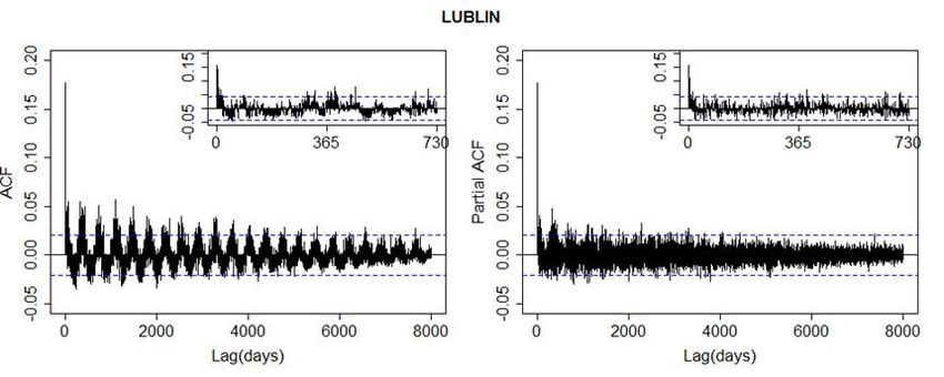
258                                                       M. MURAT et al.

Fig. 1. Autocorrelation function (ACF) and partial autocorrelation function (PACF) plots for time series of mean daily air temperature
for the studied stations. The larger plots contain lags covering the test time range of 25 years, whereas the smaller inside plots cover
a range of 2 years.
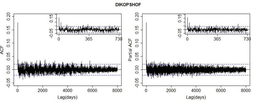
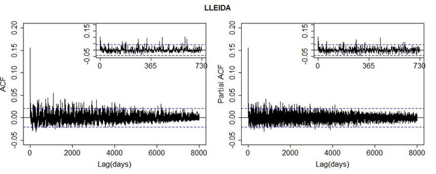
DAILY METEOROLOGICAL TIME SERIES MODELS                                                       259

Fig. 2. Autocorrelation function (ACF) and partial autocorrelation function (PACF) plots for time series of daily precipitation for the
studied stations. The larger plots contain lags covering the test time range of 25 years, whereas the smaller inside plots cover a range
of 2 years.
260                                                       M. MURAT et al.

Ta b l e 3. Forecast accuracy measures of all forecasting approaches for a daily mean air temperature time series, with p-value derived
from a Ljung-Box test

                                                                                                                             p-value
 Site             Model                          RMSE         Rank         MAE         Rank        MASE          Rank
                                                                                                                            lag=365

                  ARIMAF(3,0,1)[K=1]             3.633          1         2.915          1          0.738          1         0.038

                  RMF(1)                         3.636          2         2.917          2          0.739          2           01
 Dikopshof
                  RMP(3)                         3.715          3         2.970          3          0.752          3           01

                  SARIMA(0,0,1)(0,1,0)365        4.914          4         3.904          4          0.989          4           01

                  ARIMAF(3,0,2)[K=7]             4.536          1         3.563          2          0.768          2         0.648

                  ARIMAF(2,0,3)[K=7]             4.536          2         3.563          3          0.768          3         0.668

 Jokioinen        RMF(7)                         4.549          3         3.575          4          0.771          4           01

                  RMP(1)                         4.572          4         3.527          1          0.761          1           01

                  SARIMA(3,0,1)(0,1,0)365        5.582          4         4.340          4         0.9367          4           01

                  ARIMAF(3,0,3)[K=3]             3.023          1         2.480          2          0.753          2         0.977

                  RMF(3)                         3.024          2         2.480          3          0.753          3           01
 Lleida
                  RMP(1)                         3.061          3         2.471          1          0.751          1           01

                  SARIMA(0,0,1)(0,1,0)365        4.120          4         3.285          4          0.998          4           01

                  ARIMAF(2,0,2)[K=4]             4.156          1         3.309          1          0.734          1         0.558

                  RMF(4)                         4.173          2         3.3237         4          0.737          4           01

 Lublin           RMP(2)                         4.190          3         3.292          3          0.730          3           01

                  RMP(1)                         4.190          4         3.290          2          0.730          2           01

                  SARIMA(0,0,1)(0,1,0)365        5.331          5         4.192          5          0.930          5           01
p-value < 0.01.

applied so as to fit the created statistical models for the          the stationarity of considered series. In doing this, there
mean air temperature and the precipitation. The data from            are two different approaches: stationarity tests such as the
January 1, 2005 to December 31, 2010 were designated as              Kwiatkowski-Phillips-Schmidt-Shin (KPSS) test that con-
the test set and were used to assess the predictability accu-        sider as null hypothesis that the series is stationary, and unit
racy of the fit. This approach gives the ability to compare          root tests, such as the Dickey-Fuller test and its augmented
the effectiveness of different methods of prediction.                version, the augmented Dickey-Fuller test (ADF), or the
    Firstly, the plots of the considered series and their auto-      Phillips-Perron test (PP), for which the null hypothesis is
correlation functions (ACF) and partial autocorrelation              the contrary – that the series possesses a unit root and hence
functions (PACF), plotted in Figs 1 and 2, were examined             is not stationary. ADF and PP tests verified the stationa-
to establish the potential performances of SARIMA,                   rity of our series with p-value smaller than 0.01, which was
ARIMA, ARIMAF, RMP and RMF models for the daily                      also confirmed by the KPSS test. Therefore, the series did
air temperature and the precipitation series. In handling            not require the trend differencing, so in all ARIMA mod-
such data, the mean and the variance of the mean air tem-            els, we assumed d=0. Additionally, the ACF plots depict
perature time series are not functions of time, but rather           a sine wave and show spikes in the seasonal lags 365, 730
are constants and their covariance of the k-th term and              and 1095. This effect significantly supports the evidence
the (k + 365)-th term does not depend on time. The same              of seasonality in the data sets (except for precipitation
behaviour is shown by the precipitation time series in               in Dikopshof and Lleida). The precise study of the plots
Jokioinen and Lublin. This means that these eight series             given in Figs 1, 2b and 2d suggests the possibility of using
are stationary. Moreover, we use statistical testing to verify       SARIMA (p,d,q) (P,D,Q)m models with m = 365, D = 1,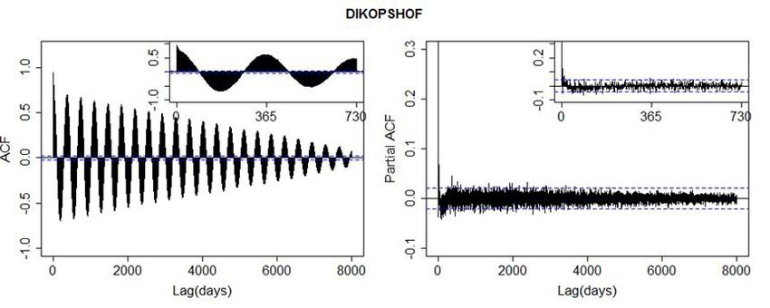
DAILY METEOROLOGICAL TIME SERIES MODELS                                                   261

Ta b l e 4. Forecast accuracy measures of all forecasting approaches for daily precipitation time series with p-value derived from
a Ljung-Box test

                                                                                                                        p-value
 Site             Model                        RMSE        Rank         MAE         Rank        MASE        Rank
                                                                                                                       lag=365

                  ARIMA(2,0,1)                 3.749         1          2.261         1         0.812         1         0.766

                  ARIMA(1,0,3)                 3.749         2          2.261         2         0.812         2         0.777
 Dikopshof
                  RMP(1)                       3.810         3          2.282         3         0.820         3           01

                  ARIMAF(0,0,3)[K=7]           3.581         1          2.227         4         0.812         4         0.469

                  ARIMAF(3,0,1)[K=7]           3.581         2          2.227         3         0.812         3         0.666

                  RMF(7)                       3.581         3          2.227         5         0.812         5           01

                  RMP(2)                       3.640         4          2.220         2         0.809         2           01
 Jokioinen
                  RMP(1)                       3.641         5          2.191         1         0.799         1           01

                  SARIMA(3,0,0)(0,1,0)365      5.903         6          2.945         6         1.074         6           01

                  ARIMA(3,0,3)                 3.479         1          1.503         2         0.863         2         0.780

                  RMP(1)                       3.905         2          1.636         3         0.940         3           01
 Lleida           RMP(4)                       3.948         3          1.425         1         0.819         1           01

                  ARIMAF(3,0,1)[K=2]           3.996         1          2.142         5         0.890         5          0.04

                  RMF(2)                       3.996         2          2.141         4         0.889         4           01

                  ARIMAF(2,0,1)[K=3]           3.999         3          2.141         2         0.889         2         0.025

                  RMF(3)                       3.999         4          2.141         3         0.889         3           01
 Lublin
                  RMP(1)                       4.057         5          2.280         6         0.946         6           01

                  RMP(3)                       4.245         6          2.038         1         0.846         1           01

                  SARIMA(1,0,1)(0,1,0)365      5.348         7          2.426         7         1.083         7           01
p-value < 0.01.
Q = 0, P = 0 and p, q changing from 0 to 3. Secondly, by          (3,0,2) [K=7], ARIMAF (3,0,3) [K=3] and ARIMAF (2,0,2)
minimising the forecast measure errors RMSE, MAE and              [K=4] models for air temperature and ARIMAF (0,0,3)
MASE, we chose the best parameters of SARIMA models               [K=7] and ARIMAF(3,0,1) [K=2] models for precipitation.
among the considered 16 models for each of the studied                The precipitation time series for Dikopshof and Lleida
sites. SARIMA (0,0,1) (0,1,0)365 and SARIMA (3,0,1)               did not show seasonal behaviour in ACF and PACF plots,
(0,1,0)365 models were selected as the most appropriate           and therefore are forecasted with use of ARIMA(p,0,q)
from all 16 tested SARIMA models for air temperature,             models with p, q changing from 0 to 3. In this case, we con-
whereas the SARIMA (3,0,0) (0,1,0)365 and the SARIMA
                                                                  sidered 16 different models for non-seasonal data sets. The
(1,0,1) (0,1,0)365 models were most appropriate from all 16
                                                                  ARIMA (2,0,2), ARIMA (1,0,3) and ARIMA (3,0,3) were
of the tested SARIMA models for precipitation.
    In order to establish ARIMAF models, we tried para-           selected as models in which forecasts can be built with the
meters p and q between 0 and 3, while the number of the           smallest RMSE, MAE or MASE – from all 16 tested ARIMA
Fourier terms K varied between 1 and 10. Therefore, for           models.
each of seasonal series, we tested 160 cases. The mo-                 To choose the best regression model, we ran the R
dels which were very close to the actual data were cho-           software with n or K varying between 1 and 10. The small-
sen by minimising the RMSE, MAE and MASE. Among                   est forecast errors gave RMP models with the polynomial
those cases, we selected ARIMAF (3,0,1) [K=1], ARIMAF             order equal to 1, 2 or 3 for air temperature and 1, 2 or 4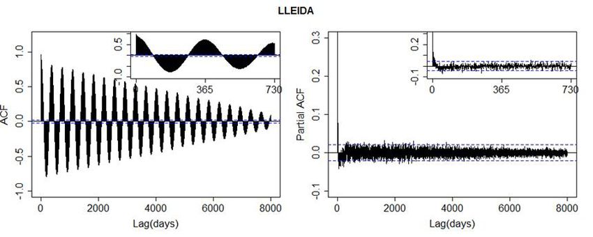
262 M. MURAT et al.
[K=1]
Air temperature (oC)
[K=3]
Air temperature (oC)
Year
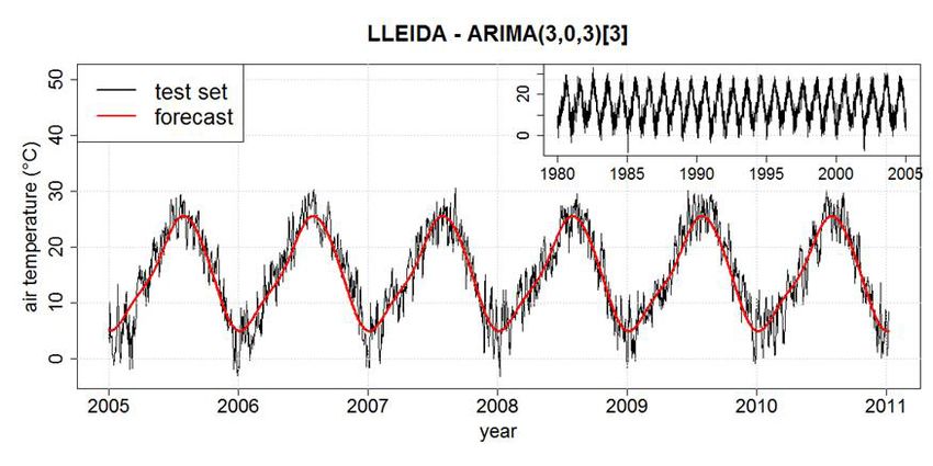
Fig. 3. Smoothed time series of air temperature and respective forecasting results with the smallest RMSE. The smaller plot inside
covers real data from the learning set.
[K=7]
Precipitation (mm)
[K=2]
Precipitation (mm)
Year
Fig. 4. Smoothed time series of precipitation and respective forecasting results with the smallest RMSE. The smaller plot inside covers
real data from the learning set.DAILY METEOROLOGICAL TIME SERIES MODELS 263
for precipitation, depending on the site. Furthermore, the ACKNOWLEDGEMENTS
smallest forecast errors were achieved for the RMF models We acknowledged the Finnish Meteorological Institute
with polynomial orders of 1, 3, 4 or 7 for air temperature (FMI) for delivering the data for Jokioinen (Venäläinen et
and 2, 3 or 7 for precipitation. al. 2005), dr. Holger Hoffmann from INRES, University of
The accuracy of the selected models for air tempera- Bonn in Germany for delivering the Dikopshof data and dr.
ture is shown in Table 3 and for precipitation (Table 4). Krzysztof Siwek from the Faculty of Earth Sciences and
From the models listed in Tables 3 and 4, we selected the
Spatial Management, Maria Curie-Skłodowska University
most adequate model which has the lowest forecast error
in Lublin, for delivering Lublin data.
when comparing predicted data using a suitable test set.
The Ljung-Box test was also performed and the obtained Conflict of interest: The Authors do not declare con-
p-values are shown in Tables 3 and 4. From the above flict of interest.
analysis, it follows that the statistical model which is the
most suitable model for the considered data sets depends on REFERENCES
the climatic zones they come from. However, the obtained Abdul-Aziz A.R., Anokye M., Kwame A., Munyakazi L., and
results show that the application of SARIMA, ARIMA, Nsowah-Nuamah N.N.N., 2013. Modeling and forecasting
ARIMAF, RMP and RMF models to an air temperature rainfall pattern in ghana as a seasonal arima process: The
and to a precipitation time series provide valuable insights case of Ashanti Region. Int. J. Humanities Social Sci., 3(3),
into the studied data structures and their components, being 224-233.
a good basis for a satisfactory prediction. Afrifa-Yamoah E., Bashiru I.I. Saeed, and Karim A., 2016.
Exemplary plots of the forecasts which produce the Sarima Modelling and Forecasting of Monthly Rainfall in
smallest RMSE and pass the Ljung-Box test are presented the Brong Ahafo Region of Ghana. World Environment,
in Figs 3 and 4. 6(1), 1-9.
Akpanta C.A., Okorie I.E., and Okoye N.N., 2015. SARIMA
CONCLUSIONS Modelling of the frequency of monthly rainfall in Umuahia,
Abia state of Nigeria. American J. Mathematics Statistics,
1. The statistical analysis shows that the daily mean 5, 82-87.
temperature data from the considered four climatic zones Ampaw E.M., Akuffo B., Opoku L.S., and Lartey S., 2013.
exhibit similar behaviour and dynamics, although some sta- Time series modeling of rainfall in new Juaben municipal-
tistical parameters differ considerably between these sites. ity of the Eastern region of Ghana. Contemporary Res.
2. Air temperature and precipitation modelling and its Business Social Sci.s, 4(8), 116-129.
forecasting pose a challenging task for handling any dai- Anitha K., Boiroju N.K., and Reddy P.R., 2014. Forecasting of
ly time series. In this study, we have shown that ARIMAF monthly mean of maximum surface air temperature in
models can efficiently capture the course of the air tempera- India. Int. J. Statistika Mathematika, 9(1), 14-19.
ture in the studied sites by producing the smallest forecast Balyani Y., Niya G.F., and Bayaat A., 2014. A study and predic-
tion of annual temperature in Shiraz using ARIMA model.
the root mean squared error and can better forecast long
J. Geographic Space, 12(38), 127-144.
seasonal time series with high frequency. Baranowski P., Krzyszczak J., Sławiński C., Hoffmann H.,
3. The best fitting model for precipitation depends on the Kozyra J., Nieróbca A., Siwek K., and Gluza A., 2015.
site. The Boreal and Continental precipitation time series Multifractal Analysis of Meteorological Time Series to
are better described by ARIMAF models, while ARIMA Assess Climate Impacts. Climate Res., 65, 39-52.
models are more appropriate for the Central Atlantic and Box G.E.P. and Jenkins G., 1970. Time Series Analysis: fore-
South Mediterranean data sets. The diagnostic checking casting and control. San Francisco, Holden-Day.
confirms the adequacy of the models. Box G.E.P., Jenkins G., and Reinsel G., 2008. Time series anal-
4. The selected models generate forecasts which are ysis. Wiley Press, New Jersey, USA.
constructed on the basis of the learn test and compared to Box G.E.P. and Tiao G.C., 1975. Intervention Analysis with
Applications to Economic and Environmental Problems.
the six-year exact values on the independent test set (out-
JASA, 70, 70-79.
of-sample accuracy forecast errors). Brockwell P.J. and Davis R.A., 1991. Time Series: Theory and
5. It was demonstrated that in practice, for obtaining rea- Methods. 2nd edition. Springer-Verlag, New York.
sonable information about the overall forecasting error, one Dabral P.P. and Murry M.Z., 2017. Modelling and Forecasting
should use more than one measure and that the best model of Rainfall Time Series Using SARIMA. Environmental
using statistical methodology could vary by changing the Processes, 1-21.
data. So, it is recommended to take into consideration all El-Mallah E.S. and Elsharkawy S.G., 2016. Time-series mode-
the time series models for any studied area and to assume ling and short term prediction of annual temperature trend
weather parameters so as to choose the suitable model. on Coast Libya using the box-Jenkins ARIMA Model.
6. Although, the chosen models cannot predict the exact Advances Res., 6(5), 1-11.
Etuk H.E., Moffat U.I., and Chims E.B., 2013. Modelling
air temperature and precipitation, they can give us informa- monthly rainfall data of portharcourt, Nigeria by seasonal
tion that helps to establish strategies for proper planning of box-Jenkins method. Int. J. Sci., 2, 60-67.
agriculture or can be used as a supplemental tool for envi- Fronzek S., Pirttioja N., Carter T.R., Bindi M., Hoffmann H.,
ronmental planning and decision-making. Palosuo T., Ruiz-Ramos M., Tao F., Trnka M., Acutis264 M. MURAT et al.
M., Asseng S., Baranowski P., Basso B., Bodin P., Buis Osarumwense O.I., 2013. Applicability of box Jenkins SARIMA
S., Cammarano D., Deligios P., Destain M.-F., Dumont model in rainfall forecasting: A case study of Port-Harcourt
B., Ewert F., Ferrise R., François L., Gaiser T., Hlavinka South South Nigeria. Canadian J. Computing in Mathe-
P., Jacquemin I., Kersebaum K.C., Kollas C., Krzyszczak matics, Natural Sciences, Engineering Medicine, 4(1), 1-4.
J., Lorite I.J., Minet J., Minguez M.I., Montesino M., Pirttioja N., Carter T.R., Fronzek S., Bindi M., Hoffmann H.,
Moriondo M., Müller C., Nendel C., Öztürk I., Perego Palosuo T., Ruiz-Ramos M., Tao F., Trnka M., Acutis M.,
A., Rodríguez A., Ruane A.C., Ruget F., Sanna M., Asseng S., Baranowski P., Basso B., Bodin P., Buis S.,
Semenov M.A., Sławiński C., Stratonovitch P., Supit I., Cammarano D., Deligios P., Destain M.-F., Dumont B.,
Waha K., Wang E., Wu L., Zhao Z., and Rötter R.P., Ewert F., Ferrise R., François L., Gaiser T., Hlavinka P.,
2018. Classifying multi-model wheat yield impact response Jacquemin I., Kersebaum K.C., Kollas C., Krzyszczak
surfaces showing sensitivity to temperature and precipita-
J., Lorite I.J., Minet J., Minguez M.I., Montesino M.,
tion change. Agricultural Systems, 159, 209-224, doi:
Moriondo M., Müller C., Nendel C., Öztürk I., Perego
10.1016/j.agsy.2017.08.004
A., Rodríguez A., Ruane A.C., Ruget F., Sanna M.,
Harvey A., 1989. Forecasting Structural Time Series Model and
the Kalman Filter. Cambridge University Press, New York. Semenov M.A., Sławiński C., Stratonovitch P., Supit I.,
Hoffmann H., Baranowski P., Krzyszczak J., Zubik M., Waha K., Wang E., Wu L., Zhao Z., and Rötter R.P.,
Sławiński C., Gaiser T., and Ewert F., 2017. Temporal 2015. Temperature and precipitation effects on wheat yield
properties of spatially aggregated meteorological time across a European transect: a crop model ensemble analysis
series. Agric. Forest Meteorol., 234, 247-257, https://doi. using impact response surfaces. Climate Research, 65,
org/10.1016/j.agrformet.2016.12.012 87-105, doi:10.3354/cr01322
Hyndman R., 2010. Forecasting with long seasonal periods. Porter J.R. and Semenov M.A., 2005. Crop responses to cli-
http://robjhyndman.com/hyndsight/longseasonality matic variation. Philosophical Trans. Royal Society B:
Hyndman R.J. and Koehler A.B., 2006. Another look at measu- Biological Sci., 360(1463), 2021-2035.
res of forecast accuracy. Int. J. Forecasting, 22(4), 679-688. Ruiz-Ramos M., Ferrise R., Rodríguez A., Lorite I.J., Bindi
Hyndman R.J., Koehler A.B., Ord J.K., and Snyder R.D., M., Carter T.R., Fronzek S., Palosuo T., Pirttioja N.,
2008. Forecasting with Exponential Smoothing: The State Baranowski P., Buis S., Cammarano D., Chen Y.,
Space Approach. Springer-Verlag Inc., New York. Dumont B., Ewert F., Gaiser T., Hlavinka P., Hoffmann
Khedhiri S., 2014. Forecasting temperature record in PEI, H., Höhn J.G., Jurecka F., Kersebaum K.C., Krzyszczak
Canada. Letters in Spatial and Resource Sciences, 9, 43-55, J., Lana M., Mechiche-Alami A., Minet J., Montesino
doi 10.1007/s12076-014-0135-x M., Nendel C., Porter J.R., Ruget F., Semenov M.A.,
Krzyszczak J., Baranowski P., Hoffmann H., Zubik M., and
Steinmetz Z., Stratonovitch P., Supit I., Tao F., Trnka M.,
Sławiński C., 2017a. Analysis of Climate Dynamics Across
de Wit A., and Rötter R.P., 2018. Adaptation response sur-
a European Transect Using a Multifractal Method, In:
faces for managing wheat under perturbed climate and CO2
Advances in Time Series Analysis and Forecasting (Eds I.
Rojas, H. Pomares, O. Valenzuela). Selected Contributions in a Mediterranean environment. Agricultural Systems,
from ITISE 2016. Springer Int. Publishing, Cham., 159, 260-274, doi: 10.1016/j.agsy.2017.01.009
doi:10.1007/978-3-319-55789-2_8. Semenov M.A. and Shewry P.R., 2011. Modelling predicts that
Krzyszczak J., Baranowski P., Zubik M., and Hoffmann H., heat stress, not drought, will increase vulnerability of wheat
2017b. Temporal scale influence on multifractal properties in Europe. Scientific Reports, 1, 66.
of agro-meteorological time series. Agric. Forest Meteorol., Sillmann J. and Roeckner E., 2008. Indices for extreme events
239, 223-235. in projections of anthropogenic climate change. Climate
Lamorski K., Pastuszka T., Krzyszczak J., Sławiński C., and Change, 86, 83-104.
Witkowska-Walczak B., 2013. Soil water dynamic mode- Tanusree D.R. and Kishore K.D., 2016. Modeling of mean tem-
ling using the physical and support vector machine methods. perature of four stations in Assam. Int. J. Advanced Res.,
Vadose Zone J., 12(4), https://doi.org/10.2136/vzj2013. 4(12), 366-370.
05.0085. Walczak R.T., Witkowska-Walczak B., and Baranowski P.,
Lobell B.D., Sibley A., and Ortiz-Monasterio J.I., 2012. 1997. Soil structure parameters in models of crop growth
Extreme heat effects on wheat senescence in India. Nature and yield prediction. Physical submodels. Int. Agrophysics,
Climate Change, 2, 186-189. 11, 111-127.
Lobell D.B., Hammer G.L., Mclean G., Messina C., Roberts Winters P.R., 1960. Forecasting sales by exponentially weighted
M.J., and Schlenker W., 2013. The critical role of extreme
moving averages. Management Sci., 6, 324-342.
heat for maize production in the United States. Nature
Venäläinen A., Tuomenvirta H., Pirinen P., and Drebs A., 2005.
Climate Change, 3, 497-501.
A basic Finnish climate data set 1961-2000-description and
Mahsin M., Akhter Y., and Begum M., 2012. Modeling rainfall
in Dhaka District of Bangladesh using time series analysis. illustration. Finnish Meteorological Institute Reports 5.
J. Mathematical Modelling Appl., 1, 67-73. Finnish Meteorological Institute, Helsinki, Finland.
Muhammet B., 2012. The analyse of precipitation and tempera- Yusof F. and Kane I.L., 2012. Modelling monthly rainfall time
ture in Afyonkarahisar (Turkey) in respect of box-Jenkins series using ETS state space and SARIMA models Int. J.
technique. J. Academic Social Sci. Studies, 5(8), 196-212. Current Res., 4(9), 195-200.
Murat M., Malinowska I., Hoffmann H., and Baranowski P., Zakaria S., Al-Ansari N., Knutsson S., and Al-Badrany T.,
2016. Statistical modeling of agrometeorological time 2012. ARIMA models for weekly rainfall in the semi-arid
series by exponential smoothing. Int. Agrophys., 30(1), Sinjar district at Iraq. J. Earth Sci. Geotechnical Eng., 2(3),
57-66. 25-55.You can also read