Giant Ragweed (Ambrosia trifida) Emergence Model Performance Evaluated in Diverse Cropping Systems - Cambridge University Press

Page created by Keith Alvarado
 
CONTINUE READING
Giant Ragweed (Ambrosia trifida) Emergence Model Performance Evaluated in Diverse Cropping Systems - Cambridge University Press
Weed Science 2018 66:36–46
       © Weed Science Society of America, 2017. This is an Open Access article, distributed under the
       terms of the Creative Commons Attribution licence (http://creativecommons.org/licenses/by/4.0/),
       which permits unrestricted re-use, distribution, and reproduction in any medium, provided the
       original work is properly cited.

                      Giant Ragweed (Ambrosia trifida) Emergence Model Performance
                                 Evaluated in Diverse Cropping Systems
                   Jared J. Goplen, Craig C. Sheaffer, Roger L. Becker, Roger D. Moon, Jeffrey A. Coulter,
                               Fritz R. Breitenbach, Lisa M. Behnken, and Jeffrey L. Gunsolus*
                   Accurate weed emergence models are valuable tools for scheduling planting, cultivation, and
                   herbicide applications. Multiple models predicting giant ragweed emergence have been developed, but
                   none have been validated in diverse crop rotation and tillage systems, which have the potential to
                   influence weed emergence patterns. This study evaluated the performance of published giant
                   ragweed emergence models across various crop rotations and spring tillage dates in southern
                   Minnesota. Across experiments, the most robust model was a mixed-effects Weibull (flexible
                   sigmoidal function) model predicting emergence in relation to hydrothermal time accumulation with a
                   base temperature of 4.4 C, a base soil matric potential of −2.5 MPa, and two random effects
                   determined by overwinter growing degree days (GDD) (10 C) and precipitation accumulated during
                   seedling recruitment. The deviations in emergence between individual plots and the fixed-effects model
                   were distinguished by the positive association between the lower horizontal asymptote (Drop) and
                   maximum daily soil temperature during seedling recruitment. This finding indicates that crops and
                   management practices that increase soil temperature will have a shorter lag phase at the start of giant
                   ragweed emergence compared with practices promoting cool soil temperatures. Thus, crops with early-
                   season crop canopies such as perennial crops and crops planted in early spring and in narrow rows will
                   likely have a slower progression of giant ragweed emergence. This research provides a valuable assess-
                   ment of published giant ragweed emergence models and illustrates that accurate emergence models can
                   be used to time field operations and improve giant ragweed control across diverse cropping systems.
                   Nomenclature: Giant ragweed, Ambrosia trifida L. AMBTR.
                   Key words: Soil temperature, weed ecology, weed emergence models, weed emergence phenology.

           Planting dates, cultivation schedules, and herbicide                                     emergence models provide a tool to optimize the
       application timing can improve weed control by being                                         timing of field operations to obtain maximum weed
       scheduled when weeds are most vulnerable (Menalled                                           control (Anderson 1994; Forcella et al. 1993). Weed
       and Schonbeck 2013). For example, spring preplant                                            emergence models can also improve our understanding
       tillage or POST herbicide applications are more                                              of abiotic factors influencing seed biology and dor-
       efficient when the number of emerged weeds is                                                mancy release. For example, emergence modeling
       maximized but weed size is small. If tillage or herbicide                                    studies have provided evidence that giant ragweed seed
       is applied too early, only a small percentage of weeds                                       dormancy is related to cold, moist conditions during
       will have emerged, whereas if either occurs too late,                                        the overwinter period, supporting previous research
       weeds may be too large to be vulnerable (Carey and                                           (Davis et al. 2013; Schutte et al. 2012).
       Kells 1995; Gunsolus 1990). Accurate weed                                                       Giant ragweed is one of the most competitive
                                                                                                    agricultural weeds in the midwestern United States
                                                                                                    row-crop production and has developed resistance to
       DOI: 10.1017/wsc.2017.38
          * First, second, third, fifth, and eighth authors: Graduate
                                                                                                    glyphosate and acetolactate synthase (ALS)-inhibitor
       Student, Professor, Professor, Professor, Associate Professor, and                           herbicides (Heap 2016; Webster et al. 1994). With
       Professor, Department of Agronomy and Plant Genetics, Uni-                                   limited herbicide options effective for giant ragweed,
       versity of Minnesota, 1991 Upper Buford Circle, St Paul, MN                                  proper herbicide application and mechanical weed
       55108; fourth author: Professor, Department of Entomology,                                   control timing is critical for maximizing weed control
       University of Minnesota, 1980 Folwell Avenue, St Paul, MN                                    efficacy (Buhler et al. 1997). Giant ragweed has been
       55108; sixth and seventh authors: Extension Educator and
       Integrated Pest Management Specialist, University of Minnesota,                              one of the earliest emerging agricultural weeds in the
       863 30th Avenue SE, Rochester, MN 55904. Corresponding                                       midwestern United States, often exhibiting a single
       author’s E-mail: gople007@umn.edu                                                            early-season flush of emergence in early spring, with
       36      •     Weed Science 66, January–February 2018
Downloaded from https://www.cambridge.org/core. IP address: 46.4.80.155, on 31 Jan 2021 at 02:04:29, subject to the Cambridge Core terms of use, available at https://www.cambridge.org/core/terms.
https://doi.org/10.1017/wsc.2017.38
90% emergence occurring by early June (Buhler et al.

                                                                                                                                                                                                                                                                        105.7c
                                                                                                                                                                                                                                                                        105.7c

                                                                                                                                                                                                                                                                                                    Abbreviations: c, curve shape parameter; drop, lower horizontal asymptote relative to upper asymptote; GDD, growing degree days; HTT, hydrothermal time; lrc, natural log
                                                                                                                                                                                                                                                        Drop
                                                                                                                                                                                                                                                                          —

                                                                                                                                                                                                                                                                          —
                                                                                                                                                                                                                                                                          —
                                                                                                                                                                                                                                                                          —
                                                                                                                                                                                                                                                                          —
            1997; Goplen et al. 2017; Werle et al. 2014),
            although some populations have developed a
            delayed, biphasic emergence pattern (Schutte et al.

                                                                                                                                                                                                                                                                        −12.7c
                                                                                                                                                                                                                                                                         −6.2c
                                                                                                                                                                                                                                                                         −8.2
                                                                                                                                                                                                                                                                         −7.4
                                                                                                                                                                                                                                                                         −7.0
                                                                                                                                                                                                                                                                         −3.5
                                                                                                                                                                                                                             Weibull model parameters

                                                                                                                                                                                                                                                                         —
                                                                                                                                                                                                                                                        lrc
            2008). Using tillage to control early-emerging weeds
            not only reduces reliance on herbicides but also

                                                                                                                                                                                                                                                                                                of the rate of increase; M, upper horizontal asymptote; STM2, soil temperature and moisture model (Spokas and Forcella 2009); z, HTT of first emergence.
            reduces weed population densities and allows POST

                                                                                                                                                                                                                                                                        1.6573
                                                                                                                                                                                                                                                                        1.2593
                                                                                                                                                                                                                                                                        1.38

                                                                                                                                                                                                                                                                        1.23
            herbicide applications to be made to smaller weeds,

                                                                                                                                                                                                                                                                        1.6
                                                                                                                                                                                                                                                                        —
                                                                                                                                                                                                                                                                        2
                                                                                                                                                                                                                                                        c
            making them more effective (Sellers et al. 2009).
               There are four publications predicting the timing

                                                                                                                                                                                                                                                                         60

                                                                                                                                                                                                                                                                          0
                                                                                                                                                                                                                                                                          0
                                                                                                                                                                                                                                                                        600
            of giant ragweed emergence based on concurrent

                                                                                                                                                                                                                                                                         —
                                                                                                                                                                                                                                                                         —
                                                                                                                                                                                                                                                                         —
                                                                                                                                                                                                                                                        Z
            weather and soil characteristics (Archer et al. 2006;
            Davis et al. 2013; Schutte et al. 2008; Werle et al.

                                                                                                                                                                                                                                                                         99.8
                                                                                                                                                                                                                                                                         99.8
            2014). All models base predictions on thermal time

                                                                                                                                                                                                                                                                         —
                                                                                                                                                                                                                                                        M

                                                                                                                                                                                                                                                                         60
                                                                                                                                                                                                                                                                         40
                                                                                                                                                                                                                                                                        100
                                                                                                                                                                                                                                                                        100
            accumulation (either growing degree days [GDD] or
            hydrothermal time [HTT]) but use different soil

                                                                                                                                                                                                                                                                                                    Models include the same fixed effects but different random effects for lrc and/or Drop determined by weather variables.
                                                                                                                                                                                                                                                                        Gompertz
                                                                                                                                                                                                                                               Equation
            temperature and moisture criteria for thermal

                                                                                                                                                                                                                                                                        Weibull
                                                                                                                                                                                                                                                                        Weibull
                                                                                                                                                                                                                                                                        Weibull
                                                                                                                                                                                                                                                                        Weibull
                                                                                                                                                                                                                                                                        Weibull
                                                                                                                                                                                                                                                                        Weibull
            time accumulation (Table 1). All models but Archer

                                                                                                                                                                                                                                               type
            et al. (2006) have used the soil temperature and

                                                                                                                      Published models predicting the emergence pattern of giant ragweed as cumulative percent emergence.a
            moisture model (STM2) (Spokas and Forcella 2009)

                                                                                                                                                                                                                                                                        (2 cm) STM2
                                                                                                                                                                                                                                                                        (2 cm) STM2
                                                                                                                                                                                                                                                                        (1 cm) STM2
                                                                                                                                                                                                                                                                        (1 cm) STM2
                                                                                                                                                                                                                                                                        (2 cm) STM2
                                                                                                                                                                                                                                                                        (2 cm) STM2
            to predict soil temperature and moisture, although

                                                                                                                                                                                                                                               Soil data

                                                                                                                                                                                                                                                                                                    Indicates model also includes random effects for the given parameter determined by weather variables.
            predictions were from different soil depths.

                                                                                                                                                                                                                                               (depth)
                                                                                                                                                                                                                                                                        (5 cm)
            The STM2 uses site-specific soil information, daily
            precipitation, and minimum and maximum air
            temperatures from a nearby weather station to pre-

                                                                                                                                                                                                                                               base (MPa)
            dict soil temperature. Although the STM2 model

                                                                                                                                                                                                                                                                        −0.15
                                                                                                                                                                                                                                                  HTT

                                                                                                                                                                                                                                                                         −2.5
                                                                                                                                                                                                                                                                         −2.5
                                                                                                                                                                                                                                                                         −10
                                                                                                                                                                                                                                                                         −30
                                                                                                                                                                                                                                                                          —
                                                                                                                                                                                                                                                                          —
            can be highly accurate, it does not account for soil
            shading as crop canopies develop (Perreault et al.
            2013; Schutte et al. 2008).
                                                                                                                                                                                                                                               base (C)
                                                                                                                                                                                                                                                GDD

               For this analysis, 11 models were derived from
                                                                                                                                                                                                                                                                         4.4
                                                                                                                                                                                                                                                                         4.4
                                                                                                                                                                                                                                                                         4.4
                                                                                                                                                                                                                                                                         2.0
                                                                                                                                                                                                                                                                         2.0
                                                                                                                                                                                                                                                                         9.0
                                                                                                                                                                                                                                                                        13.0
            four publications predicting giant ragweed emer-
            gence (Table 1). The single fixed-effect model from
            Archer et al. (2006) predicts giant ragweed emer-
                                                                                                                                                                                                                                               Prediction

                                                                                                                                                                                                                                                                        GDD
                                                                                                                                                                                                                                                                        GDD
                                                                                                                                                                                                                                                                        HTT
                                                                                                                                                                                                                                                                        HTT
                                                                                                                                                                                                                                                                        HTT
                                                                                                                                                                                                                                                                        HTT
                                                                                                                                                                                                                                                                        HTT
                                                                                                                                                                                                                                               variable

            gence with HTT using the Gompertz function:
                Y = 100  exp½6  expð0:02  HTTÞ          [1]
            where Y is cumulative percent emergence and HTT
                                                                                                                                                                                                                                                                        Fixed (common)
                                                                                                                                                                                                                                                                        Mixed (riparian)

                                                                                                                                                                                                                                                                        Fixed (postlag)
                                                                                                                                                                                                                                                                        Mixed (arable)

                                                                                                                                                                                                                                                                        Fixed (prelag)

            is the predictor variable. All other published
                                                                                                                                                                                                                                                        Model details

                                                                                                                                                                                                                                                                        Fixed (best)

            models use the Weibull function to predict giant
            ragweed emergence. The models from Schutte et al.
                                                                                                                                                                                                                                                                        Fixed

            (2008) and Werle et al. (2014) include only fixed
            effects:
                                                                    
                                                                                                                                                                                                                                                                        2,4,5,6,7,8b

               Y = M  1  exp½ð expðlrcÞÞ  ðGDD or HTT  z Þ ^ c 
                                                                                                                                                                                                                                                        Model no.

                                                                                               [2]
                                                                                                                                                                                                                                                                              1

                                                                                                                                                                                                                                                                              3
                                                                                                                                                                                                                                                                              9
                                                                                                                                                                                                                                                                              9
                                                                                                                                                                                                                                                                             10
                                                                                                                                                                                                                                                                             11

            where Y is cumulative percent emergence, M is the
            upper horizontal asymptote, lrc is the natural log of
            the rate of increase, GDD or HTT is the predictor
                                                                                                                                                                                                                                                                        Schutte et al. (2008)
                                                                                                                                                                                                                                                                        Schutte et al. (2008)
                                                                                                                                                                                                                                                                        Archer et al. (2006)

                                                                                                                                                                                                                                                                        Werle et al. (2014)
                                                                                                                                                                                                                                                                        Werle et al. (2014)

            variable, z is the time of first emergence, and c is the
                                                                                                                                                                                                                                                                        Davis et al. (2013)
                                                                                                                                                                                                                                                                        Davis et al. (2013)

            curve shape parameter. The fixed-effects models
            have model parameters that are fixed across all
            locations, years, and changing weather conditions,
                                                                                                                                       Table 1.

                                                                                                                                                                                                                                                        Citation

            with model parameters presented in Table 1. Davis
                                                                                                                                                                                                                                                                                                  b
                                                                                                                                                                                                                                                                                                a

                                                                                                                                                                                                                                                                                                  c

            et al. (2013) included an additional fixed effect for
                                                                                                        Goplen et al.: Giant ragweed emergence models                                                                                                                                                                                                                                                                                                                           •   37
Downloaded from https://www.cambridge.org/core. IP address: 46.4.80.155, on 31 Jan 2021 at 02:04:29, subject to the Cambridge Core terms of use, available at https://www.cambridge.org/core/terms.
https://doi.org/10.1017/wsc.2017.38
a lower horizontal asymptote (Drop) to the Weibull                                           were fixed-effects Weibull functions with GDD
       function, as in Equation 3:                                                                  predictor variables but with different base tempera-
                                                                                                    tures for GDD calculation and different model
          Y = M  ðDrop + dropÞ  exp½ðexpðlrc + lrc ÞÞ  ðHTTÞ ^ c                     [3]
                                                                                                    parameters (Table 1).
       as well as random effects for drop and lrc, which were                                          The models from Davis et al. (2013) included
       determined by their published associations with                                              two mixed-effects Weibull functions with an HTT
       weather variables and were different for each site-                                          predictor variable designed for either arable or
       year (Equation 3). The terms for drop included by                                            riparian accessions of giant ragweed. Each model had
       Davis et al. (2013) determine how much lower the                                             different fixed-effect parameters for lrc and c but the
       lower horizontal asymptote is relative to the upper                                          same fixed-effect parameters for M and Drop.
       horizontal asymptote, which had a fixed value of                                             In addition to the fixed effects, these models inclu-
       99.8 for all models derived from Davis et al. (2013)                                         ded random effects for lrc and drop. Davis et al.
       (Table 1). In Equation 3, Drop and drop are the                                              (2013) found that overwinter GDD (10 C) and
       fixed and random effects, respectively, for the lower                                        rainfall during seedling recruitment were both
       horizontal asymptote relative to the upper asymp-                                            negatively associated with the random effect lrc and
       tote, and lrc and lrc are the fixed and random effects,                                      that rainfall during seedling recruitment was nega-
       respectively, for the natural log of the rate of                                             tively associated with the random effect drop. Davis
       increase. Fixed-effect parameters for all models are                                         et al. (2013) concluded that these weather variables
       presented in Table 1, while random-effect para-                                              are what influenced deviations from the fixed-
       meters were estimated from their associations with                                           effects-only models, and therefore can be used to
       weather variables found in Davis et al. (2013).                                              improve model predictions in years or locations with
          The model from Schutte et al. (2008) was a two-                                           differing weather conditions. The associations
       part model, with a pre– and post–lag phase com-                                              found by Davis et al. (2013) between weather
       ponent based on the Weibull function, designed to                                            variables and random effects for lrc and drop were
       predict emergence of giant ragweed with a biphasic                                           used to predict the random-effect parameters for
       emergence pattern like the populations found in                                              each site-year of this study, which is how Models 4
       Ohio. Both phases of this model had an HTT                                                   to 8 were derived in Table 2. All giant ragweed
       predictor variable but different base soil matric                                            populations in our study were from arable acces-
       potential and model parameters for each phase                                                sions, so arable accession Model 2 was used as a
       (Table 1). Werle et al. (2014) presented two models,                                         basis for the mixed-effects Models 4 to 8 (Tables 1
       one of which was the best giant ragweed emergence                                            and 2). Models 4 to 8 had the same fixed effects as
       model in their study and another which was a                                                 arable accession Model 2 but different random
       common model among other weed species evaluated                                              effects for each site-year that were predicted from
       in their study. Both models from Werle et al. (2014)                                         Davis et al. (2013).

       Table 2.       Summary of model performance criteria ordered by model performance across experiments and site-years (n = 1,586).a
                                                 GDD base             HTT base
                                                Temperature           moisture          Random
       Model no.         Model                    —C—                 —MPa—             effects                   AICc             wi         RMSE           r          A         CCC
       8                 Davis arable                  4.4                −2.5          W lrc + P drop           −5,445        >0.999          0.18        0.87        0.97        0.85
       5                 Davis arable                  4.4                −2.5          W lrc                    −5,383
Davis et al. (2013) and Schutte et al. (2008)                                            Tillage Experiments. Two additional field experi-
            developed giant ragweed emergence models by                                                  ments were conducted in 2015 near Rochester, MN
            evaluating giant ragweed emergence with no sur-                                              (43.91°N, 92.56°W) and at the University of
            rounding vegetation, while Werle et al. (2014)                                               Minnesota Rosemount Research and Outreach Center
            developed emergence models in an experiment plan-                                            near Rosemount, MN (44.70°N, 93.08°W) (Goplen
            ted to soybean [Glycine max (L.) Merr.] that achieved                                        2017). Both sites had naturally occurring giant rag-
            a crop canopy after the majority of giant ragweed                                            weed resistant to glyphosate, and at Rochester, MN,
            emergence had occurred. Although Schutte et al.                                              giant ragweed was also resistant to ALS-inhibitor
            (2008) validated their model in both no-tillage and                                          herbicides. Each experiment had six tillage treatments
            tilled conditions, the type of crop, crop residue, and                                       arranged in a randomized complete block design with
            tillage influences the soil environment, which can alter                                     four replications. The tillage treatments included
            giant ragweed emergence. Since all published emer-                                           multiple dates of spring tillage timed relative to the
            gence models were constructed in either fallow or                                            initiation of giant ragweed emergence. Treatments
            annual row-crop systems, it is likely that model per-                                        included tillage with a field cultivator at a depth of
            formance, or how closely a model predicts actual giant                                       10 cm at emergence onset; at 14, 28, and 42 d after
            ragweed emergence, will decrease in perennial crops or                                       emergence onset; at emergence onset and repeated at
            crops planted early in the season and in narrow rows,                                        28 d after onset; and no tillage. At Rochester, MN,
            because they affect early-season soil temperature and                                        two replications were in oat stubble that had no fall
            moisture (Liebman and Dyck 1993). Giant ragweed                                              tillage, and the other two replications were in
            emergence has been shown to be prolonged with                                                fall chisel-plowed corn stubble. At Rosemount, MN,
            less total seedling recruitment in established alfalfa                                       all replications took place in fall chisel-plowed
            (Medicago sativa L.), which was attributed to lower soil                                     soybean stubble. Plots at Rosemount, MN, were 3
            temperatures being less conducive to giant ragweed                                           by 6 m, and plots at Rochester, MN were 3.7 by 6 m
            recruitment (Goplen et al. 2017; Wortman et al.                                              to accommodate equipment size. Ten 0.09-m2
            2012). It is important to validate the applicability of                                      quadrats were placed in each plot. Giant ragweed
            giant ragweed emergence models in diverse cropping                                           emergence was monitored by counting and removing
            systems to identify reliable models for timing field                                         emerged seedlings in each quadrat on a weekly
            operations. The objectives of this research were to                                          basis, starting at emergence onset and continuing for
            evaluate the performance of published giant ragweed                                          at least 10 wk or until emergence ceased. All emer-
            emergence models across contrasting cropping sys-                                            gence data were converted to a cumulative percentage
            tems, and determine biotic or abiotic factors associated                                     of giant ragweed that emerged each week. These
            with deviations in emergence model predictions.                                              tillage timing experiments contributed data from
                                                                                                         48 experimental units for analysis of giant ragweed
                                                                                                         emergence models.
                                 Materials and Methods
            Crop Rotation Experiments. Two field experi-                                                 Environmental Effects. Daily precipitation and
            ments were initiated in 2012 and 2013 at separate                                            minimum and maximum air temperatures were
            sites with naturally occurring giant ragweed resistant                                       obtained from the National Weather Service station
            to glyphosate and ALS-inhibitor herbicides near                                              within 5 km of each study location. Weather data
            Rochester, MN (43.91°N, 92.56°W). Crop manage-                                               from each weather station were used to predict daily
            ment details are outlined in Goplen et al. (2017) and                                        soil temperature (C) and moisture (MPa) at 1-, 2-,
            consisted of six 3-yr crop rotation treatments applied                                       and 5-cm depths using STM2 (Spokas and Forcella
            in a randomized complete block design with four                                              2009). The STM2 predictions were based on daily
            replications. Crops in the rotations were corn                                               maximum and minimum air temperature, daily
            (Zea mays L.), soybean, wheat (Triticum aestivum L.),                                        precipitation, soil properties (sand, silt, clay, and
            and alfalfa. Rotations were continuous corn, soybean–                                        organic matter), latitude, longitude, and elevation.
            corn–corn, corn–soybean–corn, soybean–wheat–corn,                                               Thermal time for each giant ragweed emergence
            soybean–alfalfa–corn, and alfalfa–alfalfa–corn. Giant                                        model was calculated using the method specified in
            ragweed emergence was monitored on a weekly basis                                            the respective publication. All emergence models
            with emergence data from a total of 120 experimental                                         calculated GDD as:
            units over 3 yr being used for emergence model                                                                             XS2 ðTmax + Tmin Þ
            analysis, as weekly emergence data were not collected                                                       GDD =                                           Tb               [4]
            in 2012.                                                                                                                         S1            2
                                                                                                        Goplen et al.: Giant ragweed emergence models                                 •    39
Downloaded from https://www.cambridge.org/core. IP address: 46.4.80.155, on 31 Jan 2021 at 02:04:29, subject to the Cambridge Core terms of use, available at https://www.cambridge.org/core/terms.
https://doi.org/10.1017/wsc.2017.38
where Tmax is maximum daily soil temperature, Tmin                                           candidate models (Anderson 2008; Burnham and
       is minimum daily soil temperature, Tb is base                                                Anderson 2002; Hoeting et al. 1999). Akaike weights
       temperature for GDD calculation presented in                                                 (wi) closer to 1 indicate stronger support for a candi-
       Table 1, and S1 and S2 are beginning and ending                                              date model given the data. This methodology has been
       dates for the specific model, respectively. For models                                       used in previous giant ragweed emergence modeling
       using hydrothermal time (HTT) to predict emer-                                               studies to select the best-fitting predictive model while
       gence, HTT was calculated as:                                                                minimizing the number of parameters (Davis et al.
                               XS2                                                                  2013; Werle et al. 2014).
                      HTT =       S1 H
                                      θ GDD               [5]                                          Since AICc will rank models even if none perform
                                                                                                    well, it is recommended that additional performance
       where GDD were calculated according to Equation 4,                                           criteria be used (Anderson 2008; Kobayashi and
       θH = 1 when soil matric potential was in the model’s                                         Salam 2000; Legates and McCabe 1999; Meek et al.
       designated interval, and θH = 0 when soil matric                                             2009; Tedeschi 2006). Following earlier methods
       potential was not in the model’s designated interval                                         (Schutte et al. 2008; Werle et al. 2014), goodness of
       (Table 1). Therefore, thermal time was only accumu-                                          fit for each model was analyzed using root mean
       lated when soil moisture was in the designated                                               square error (RMSE) and the concordance cor-
       interval. Soil temperature at the 5-cm depth was                                             relation coefficient (CCC) to provide measures of
       recorded hourly in plots from all experiments using                                          giant ragweed emergence model precision and
       temperature sensors (Hobo® Water Temp Pro v2,                                                accuracy. The RMSE was calculated to estimate
       Bourne, MA). Soil temperature data from temperature                                          model prediction accuracy and is recommended
       sensors were used to evaluate STM2 accuracy and                                              when using AICc model selection methods
       explore deviations from emergence predictions in crop                                        (Anderson 2008; Legates and McCabe 1999;
       rotation and tillage timing treatments.                                                      Tedeschi 2006). The RMSE is calculated as:
                                                                                                                            sffiffiffiffiffiffiffiffiffiffiffiffiffiffiffiffiffiffiffiffiffiffiffiffiffiffiffiffiffiffiffi
       Statistical Analysis. Measures of model perfor-                                                                         Pn                         2
       mance in our study were based on comparison                                                                                 i = 1 ðOi  Pi Þ
                                                                                                                  RMSE =                                     [8]
       between observed and predicted values for cumulative                                                                                n
       percent emergence of giant ragweed across the entire                                         where Oi and Pi are the observed and predicted values
       seedling recruitment period. Corrected Akaike’s                                              of the cumulative percentage of giant ragweed
       information criterion (AICc) was used to evaluate                                            emerged, respectively, and n is the number of
       competing giant ragweed emergence models across                                              comparisons. The CCC was calculated as an additional
       experiments. This criterion includes a correction for                                        model performance measure, since it provides a
       sample size and is recommended in practice over                                              measure of precision and accuracy (Mitchell 1997).
       traditional AIC (Anderson 2008; Hurvich and Tsai                                             The CCC is:
       1989; Sugiura 1978). It is based on the minimization
       of maximum-likelihood criterion and is calculated as:                                                             CCC = rA                     [9]
                                  2K ðK + 1Þ                                                    which is the product of Pearson’s correlation
               AICc = 2log L θ^ j x +                     [6]                                      coefficient (r) and accuracy (A). Accuracy (A) is a
                                            nK 1
                                                                                                    bias correction factor calculated as:
       where the first term involves the log-likelihood of the
       model, given the data, while the second term penalizes                                                                4sx sy  rðsy2 + sx2 Þ
       a model for K additional parameters and sample size of                                                       A=                           2                             [10]
       n. Models with lower values of AICc indicate they                                                               ð2  r Þ sy2 + sx2 + μy μx
       better represent reality given the data. Akaike weights
       (wi) were calculated from the AICc values for the 11                                         where sx is mean deviation x from μx , sy is mean
       models to determine the probability that a given model                                       deviation y from μy, μy is the mean of the observed
       is the best descriptor of reality among the candidate                                        values, and μx is the mean of the model prediction.
       models. Akaike weights were calculated as:                                                   The CCC can range from −1 to 1, with values near 1
                                                                                                    indicating better-fitting models (Meek et al. 2009).
                                                 e 1=2Δi                                              Deviations from the best giant ragweed emer-
                                   wi = PR                                               [7]        gence model were analyzed to determine whether
                                                         1=2Δr
                                                r =1 e                                              they were associated with crop rotation or tillage
       where Δi is the AICc difference between the top model                                        treatments or with specific soil temperature condi-
       and the ith alternative, and R is the number of                                              tions. Since the best giant ragweed emergence model
       40      •     Weed Science 66, January–February 2018
Downloaded from https://www.cambridge.org/core. IP address: 46.4.80.155, on 31 Jan 2021 at 02:04:29, subject to the Cambridge Core terms of use, available at https://www.cambridge.org/core/terms.
https://doi.org/10.1017/wsc.2017.38
was from a mixed-effects model, random effects were                                          The more rapid progression of giant ragweed
            fit to the observed data using maximum-likelihood                                            emergence following colder overwinter periods
            methods in each treatment and site-year as done by                                           observed in this study has been shown to be related
            Davis et al. (2013). Regression analyses were then                                           to greater dormancy loss following cold and moist
            performed to determine the relationship between                                              conditions (Ballard et al. 1996; Davis et al. 2013;
            fitted random effects, which were the dependent                                              Schutte et al. 2012). Overwinter GDD (10 C)
            variables, and crop rotation and tillage treatments                                          accumulated in this study ranged from 20 to 67
            and observed soil temperature data. All analyses were                                        GDD (10 C), which was comparable to the coldest
            performed using R v. 3.1.3 (R Foundation for                                                 overwinter periods observed by Davis et al. (2013),
            Statistical Computing, Vienna, Austria).                                                     which ranged from 0 to 300 GDD (10 C). This
                                                                                                         resulted in more rapid emergence predictions in all
                                                                                                         site-years of our study compared with the fixed-
                                Results and Discussion                                                   effects-only Model 2 (Figure 1). Davis et al. (2013)
            Giant Ragweed Emergence. Giant ragweed                                                       also found an association (r = −0.39, P = 0.10)
            emerged early in the growing season in all experi-                                           between drop and precipitation accumulated during
            ments, where on average 90% of giant ragweed                                                 seedling recruitment, which was used to predict drop
            emergence occurred on May 29 and June 4 in the                                               in Model 8 (AS Davis, personal communication).
            tillage and crop rotation experiments, respectively                                          The negative association between drop and pre-
            (Goplen 2017; Goplen et al. 2017). Crop rotations                                            cipitation during seedling recruitment indicates that
            with annual crops had similar giant ragweed emer-                                            smaller values for drop occur when there is greater
            gence phenology, whereas emergence was slightly                                              precipitation during seedling recruitment, resulting
            prolonged in established alfalfa, likely due to the                                          in an extended lag phase when there is greater pre-
            prominent early-season crop canopy (Goplen et al.                                            cipitation during seedling recruitment. Compared
            2017). Tillage treatment reduced giant ragweed                                               with Model 2, including the random effects W lrc
            emergence the week following tillage, likely because                                         and P drop in Model 8 improved model performance
            tillage disrupted germinating seedlings and                                                  by reducing RMSE by 0.04 and increasing CCC by
            prevented them from emerging the week following                                              0.03 (Figure 1; Table 2). The improved emergence
            tillage (Goplen 2017). Tillage treatments had similar                                        predictions with Model 8 compared with the fixed-
            levels of total giant ragweed emergence (P = 0.466),                                         effects-only Model 2 confirm the findings of Davis
            however, indicating that tillage did not stimulate or                                        et al. (2013) that random effects for lrc and drop
            suppress total giant ragweed emergence.                                                      describe deviations from the fixed-effects-only
                                                                                                         Model 2 (Table 2).
            Model Performance. Across all experiments and                                                   Model 5, a mixed-effects model derived from
            site-years, giant ragweed emergence was best fit by                                          Davis et al. (2013) with fixed effects and a single
            Model 8, a mixed-effects model derived from the                                              random effect for W lrc, was the second best
            arable accession model of Davis et al. (2013)                                                performing giant ragweed emergence model evaluated
            (Tables 1 and 2). Model 8 had the lowest AICc,                                               in this study. The random effect in Model 5 included
            greatest Akaike weight (wi), lowest RMSE, and                                                the same random effect for lrc (W lrc) included in
            greatest CCC among candidate models, although it                                             Model 8 based on overwinter GDD (10 C), but did
            was only marginally better than Model 5, indicating                                          not include the random effect for drop (P drop).
            that it had the best fit of emergence across diverse                                         Including only W lrc in Model 5 still resulted in
            cropping systems in this study (Table 2). Model 8                                            better model performance than the fixed-effects-only
            included the fixed effects specified in Table 1, and                                         Model 2 and had nearly the same measures of RMSE
            random effects determined by overwinter GDD                                                  and CCC as the top model. Model 5 had an Akaike
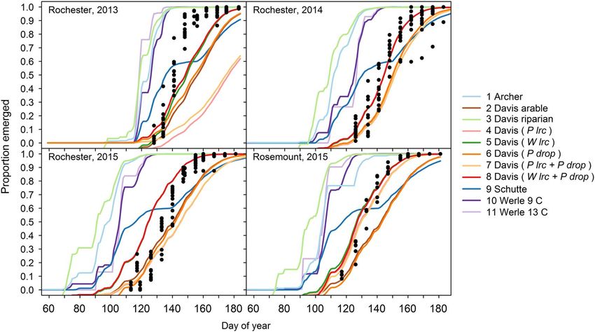
            (10 C) accumulated from October through March                                                weight (wi) of
Figure 1. Predicted cumulative giant ragweed emergence by model in relation to observed mean cumulative emergence in each
       experimental treatment. Random effects included in the Davis et al. (2013) arable-accession mixed-effects models are shown in
       parentheses. Abbreviations: P drop, drop determined by precipitation during recruitment; P lrc, natural log of the rate of increase
       determined by precipitation during recruitment; W lrc, natural log of the rate of increase determined by winter GDD (10 C)
       accumulated from October to March.

       accumulated during seedling recruitment (P drop),                                            are unknown until the end of seedling recruitment,
       which resulted in model performance measures only                                            meaning real-time emergence predictions will
       marginally better than the fixed-effects-only                                                require recalculation of random-effect parameters
       Model 2 (Table 2). Models 4 and 7 had a random                                               as precipitation accumulates or use of historical
       effect for lrc determined by precipitation during                                            averages and weather forecasts to predict random-
       seedling recruitment (P lrc), and Model 7 included                                           effect parameters.
       an additional random effect for drop based on                                                   Model 9 was derived to model emergence of giant
       precipitation accumulated during seedling recruit-                                           ragweed with a biphasic emergence pattern in Ohio
       ment (P drop). Random effects for lrc and drop were                                          (Schutte et al. 2008) and was among the top-
       determined from Davis et al. (2013) by the negative                                          performing models in our study. In our study, giant
       associations between lrc and drop and precipitation                                          ragweed emergence generally occurred after the early
       accumulated during seedling recruitment. Among all                                           flush but before the late flush of emergence predicted
       models derived from Davis et al. (2013), the two                                             by Model 9. This monophasic emergence pattern
       best-fitting models across our experiments included                                          aligning between the two flushes of emergence
       a random effect for lrc determined by overwinter                                             predicted by Model 9 indicates that giant ragweed
       GDD (Models 5 and 8), while the worst-fitting                                                populations in Minnesota have not diverged in their
       models determined the random effect for lrc by                                               emergence timing as populations found in Ohio have
       precipitation accumulated during seedling recruit-                                           done (Figure 1).
       ment (Models 4 and 7). These findings indicate that                                             Across the crop rotation and tillage timing experi-
       lrc is more closely associated with overwinter GDD                                           ments, soil temperature at the 5-cm depth predicted
       (10 C) than precipitation during seedling recruit-                                           by the STM2 was associated with observed soil
       ment (Table 2). Random-effect model parameters                                               temperature (R2 = 0.88, P < 0.001) (Figure 2).
       based on overwinter GDD (10 C) are also easier to                                            Although the observed and predicted soil temperatures
       use in making real-time emergence predictions,                                               were associated, the STM2 had a mean bias of 2.9 C,
       because random effects predicted from overwinter                                             indicating that the STM2 predicted soil temperature to
       GDD (10 C) are known prior to giant ragweed                                                  be 2.9 C warmer on average than what was observed.
       recruitment. Random-effect parameters based on                                               The 2.9 C bias of STM2 temperature predictions
       precipitation during the seedling recruitment period                                         caused predicted thermal time to accumulate faster

       42      •     Weed Science 66, January–February 2018
Downloaded from https://www.cambridge.org/core. IP address: 46.4.80.155, on 31 Jan 2021 at 02:04:29, subject to the Cambridge Core terms of use, available at https://www.cambridge.org/core/terms.
https://doi.org/10.1017/wsc.2017.38
Soil Temperature Associations. The mixed-
                                                                                                         effects models derived by Davis et al. (2013) pro-
                                                                                                         vide a versatile framework to study giant ragweed
                                                                                                         emergence, since unexplained model deviations can
                                                                                                         be attributed to environmental variation (Luschei
                                                                                                         and Jackson 2005). The associations found by Davis
                                                                                                         et al. (2013) allowed the derivation of mixed-effects
                                                                                                         Models 4 through 8 in our study. Using this same
                                                                                                         approach, new estimates of the random effects drop
                                                                                                         and lrc were determined for the arable accession
                                                                                                         model (Model 2) from Davis et al. (2013) for each
                                                                                                         site-year and treatment combination in our study.
                                                                                                         Regression analyses were performed to determine
                                                                                                         associations between random effects and experi-
                                                                                                         mental treatments and soil temperature (average
            Figure 2. Daily average soil temperature at the 5-cm depth                                   daily minimum, maximum, mean, and fluctuation
            predicted by the soil temperature and moisture model                                         in temperature for various intervals during the
            (STM2) during the crop rotation and tillage timing                                           seedling recruitment period). Neither crop rotation
            experiments relative to observed soil temperature. The solid
            1:1 line (y = x) indicates perfect agreement between observed
                                                                                                         sequence nor tillage timing treatments were asso-
            and predicted soil temperature, while the dotted line indicates                              ciated with the estimated random effects drop or lrc
            the fitted regression equation (y = 0.96x − 2.1, R2 = 0.88,                                  (R2 = 0.07 to 0.42, P = 0.55 to 0.99). There also
            P < 0.001) between observed and predicted soil temperature.                                  were no associations between the estimated random
                                                                                                         effects for lrc and soil temperature variables
                                                                                                         (R2 = 0.01 to 0.07, P = 0.17 to 0.99). All soil
            than what actually occurred and contributed to                                               temperature variables analyzed were positively asso-
            premature giant ragweed emergence predictions for                                            ciated with the estimated random effects for drop
            Models 1, 3, 10, and 11 in all site-years (Figure 1).                                        (R2 = 0.24 to 0.72, P < 0.001 to 0.006), meaning
            This finding is similar to that of Perreault et al. (2013),                                  warmer soil temperature variables or greater tem-
            who reported a mean bias of 2.5 C for STM2 on                                                perature fluctuations had greater fitted random
            loamy soils similar to soils at both of our study                                            effects for drop. The soil temperature variable most
            locations. The mean bias of the STM2 among crop                                              strongly associated with the fitted random effect for
            rotation and tillage timing treatments ranged from 1.7                                       drop was the maximum daily soil temperature during
            to 3.9 C. Established alfalfa and wheat had the greatest                                     the entire seedling recruitment period (R2 = 0.72,
            mean bias values of 3.8 and 3.9 C, respectively, while                                       P < 0.001). This relationship indicates that greater
            soybean planted into soybean stubble had the lowest                                          maximum soil temperatures during seedling
            mean bias value of 1.7 C. The STM2 does not account                                          recruitment were associated with greater fitted ran-
            for changes in crop canopy during the growing season                                         dom effects for drop, the term representing the lower
            (Perreault et al. 2013), which likely explains why the                                       horizontal asymptote of the Weibull function
            STM2 predictions had a greater bias in established                                           (Figure 3). A greater random effect for drop equates
            alfalfa and wheat, which were established earlier and in                                     to a shorter lag period at the start of giant ragweed
            narrower rows compared with corn and soybean. The                                            emergence.
            STM2 model was likely more accurate in previous                                                 Observed average daily soil temperature fluctua-
            giant ragweed emergence modeling studies, since they                                         tion during the entire seedling recruitment period
            were developed with little or no canopy coverage                                             was the second most significant association with the
            (Archer et al. 2006; Davis et al. 2013; Schutte et al.                                       estimated random effects for drop (R2 = 0.70,
            2008; Werle et al. 2014). Including a 2.9 C mean bias                                        P < 0.001) (Figure 3). It is possible that either the
            correction factor for STM2 predictions decreased the                                         amplitude or number of temperature fluctuations
            RMSE of Models 1, 3, 10, and 11 by 0.06, 0.03,                                               influences giant ragweed emergence rather than
            0.09, and 0.08, respectively. However, including the                                         maximum soil temperature, as shown for other weed
            mean bias correction factor increased the RMSE of                                            species including johnsongrass [Sorghum halpense
            Model 8 by 0.02, indicating that Model 8 without a                                           (L.) Pers.] and large crabgrass [Digitaria sanguinalis
            bias correction was still the best among all models                                          (L.) Scop.] (Benech Arnold et al. 1990a, 1990b;
            evaluated.                                                                                   Forcella et al. 2000; King and Oliver 1994). Daily
                                                                                                        Goplen et al.: Giant ragweed emergence models                                 •    43
Downloaded from https://www.cambridge.org/core. IP address: 46.4.80.155, on 31 Jan 2021 at 02:04:29, subject to the Cambridge Core terms of use, available at https://www.cambridge.org/core/terms.
https://doi.org/10.1017/wsc.2017.38
Figure 3. Association between the estimated random effects of drop and (a) mean maximum daily temperature observed at a 5-cm soil
       depth during the seedling recruitment period and (b) mean daily temperature fluctuation at a 5-cm soil depth during seedling
       recruitment.

       maximum soil temperature was the primary factor                                              crops established early in the growing season that limit
       influencing daily temperature fluctuation, as evi-                                           soil temperature, such as small grains or cover crops
       denced by the strong association between the two                                             (Zhang et al. 2009), although this was not shown to
       variables (r = 0.98, P < 0.001), indicating that                                             be the case for wheat (Goplen et al. 2017). It is also
       greater daily maximum soil temperature is more                                               possible that crop management practices maintaining
       influential on daily soil temperature fluctuation than                                       increased soil residue associated with conservation
       daily minimum soil temperature, which has been                                               tillage will have similar effects on giant ragweed
       reported previously (Perreault et al. 2013). These                                           emergence, since they can also affect soil temperature
       findings indicate that giant ragweed emergence will                                          (Griffith et al. 1973; Kladivko et al. 1986).
       have a shorter lag phase at the start of emergence in                                            Model 8, a mixed-effects model derived from
       environments with greater maximum daily soil                                                 Davis et al. (2013) that included random effects for
       temperature and corresponding greater soil tempera-                                          drop and lrc based on precipitation accumulated
       ture fluctuation. Davis et al. (2013) stated that the                                        during seedling recruitment and overwinter GDD
       associations they found between random effects for                                           (10 C), respectively, was the model that most
       lrc and precipitation accumulated during seedling                                            accurately predicted giant ragweed emergence across
       recruitment may have been caused by increased                                                crop rotations and spring tillage dates. The top four
       cloud cover accompanying increased precipitation.                                            models that best fit giant ragweed emergence in the
       Cloud cover and precipitation can limit maximum                                              present study originated from Davis et al. (2013),
       daily soil temperature, and since soil temperature                                           with the top two models including random effects
       was not directly measured in Davis et al. (2013), it is                                      predicted by overwinter GDD (10 C). This is
       possible that the association between random effects                                         supported by studies of giant ragweed seed dor-
       and precipitation during seedling recruitment found                                          mancy, which have found that cold and moist
       in Davis et al. (2013) was driven by maximum daily                                           conditions during winter enhance seed dormancy
       soil temperature or daily temperature fluctuation, as                                        release (Ballard et al. 1996; Schutte et al. 2012).
       found in the present study.                                                                      This is the first study to verify the utility of
          The positive association between random effects for                                       previously published giant ragweed emergence
       drop and mean maximum daily soil temperature                                                 models under a diversity of crop management
       supports the findings of Goplen et al. (2017), in                                            practices and supports previous research showing
       which giant ragweed emergence extended later into                                            that giant ragweed emergence is affected by winter
       the growing season in established alfalfa compared                                           weather. This research also suggests that crops such
       with annual crops. The extended emergence was                                                as alfalfa, small grains, and cover crops, which have
       likely due to lower soil temperatures causing a longer                                       lower soil temperature during seedling recruitment
       initial lag period in emergence. Longer initial lag                                          compared with annual row crops, will have a
       periods in emergence could also be expected in other                                         longer lag phase at the initiation of giant ragweed
       44      •     Weed Science 66, January–February 2018
Downloaded from https://www.cambridge.org/core. IP address: 46.4.80.155, on 31 Jan 2021 at 02:04:29, subject to the Cambridge Core terms of use, available at https://www.cambridge.org/core/terms.
https://doi.org/10.1017/wsc.2017.38
emergence, potentially extending emergence later into                                        Forcella F, Eradat-Oskoui K, Wagner SW (1993) Application of
            the growing season. The delay in emergence may                                                  weed seedbank ecology to low-input crop management. Ecol
            provide weed control benefits, as later-emerged giant                                           Appl 3:74–83
                                                                                                         Goplen JJ (2017) Emergence modeling and economics of
            ragweed will be subjected to increased competition                                              managing herbicide-resistant giant ragweed (Ambrosia trifida)
            with established crops. As herbicide-resistant giant                                            with crop rotation. Ph.D. dissertation. Minneapolis, MN:
            ragweed continues to be problematic, robust emer-                                               University of Minnesota. 73 p
            gence model predictions will be increasingly important                                       Goplen JJ, Sheaffer CC, Becker RL, Coulter JA, Breitenbach FR,
            to optimize planting, tillage, and herbicide application                                        Behnken LM, Johnson GA, Gunsolus JL (2017) Seed bank
                                                                                                            depletion and emergence patterns of giant ragweed (Ambrosia
            dates in a variety of crop management systems to                                                trifida) in Minnesota cropping systems. Weed Sci 65:52–60
            improve giant ragweed control.                                                               Griffith DR, Mannering JV, Galloway HM, Parsons SD, Richey
                                                                                                            CB (1973) Effect of eight tillage-planting systems on soil
                                    Acknowledgments                                                         temperature, percent stand, plant growth, and yield of corn on
                                                                                                            five Indiana soils. Agron J 65:321–326
              This research was funded by the Monsanto Graduate                                          Gunsolus JL (1990) Mechanical and cultural weed control in
            Fellowship, the Rapid Agricultural Response Fund of the                                         corn and soybeans. Am J Alternative Agr 5:114–119
                                                                                                         Heap I (2016) The International Survey of Herbicide-Resistant
            University of Minnesota Agricultural Experiment Station,                                        Weeds. http://www.weedscience.org. Accessed: December 6,
            and the Torske Klubben Graduate Fellowship. The authors                                         2016
            express appreciation to numerous faculty, staff members,                                     Hoeting JA, Madigan D, Raftery AE, Volinsky CT (1999)
            and students for their assistance, in particular Adam Davis,                                    Bayesian model averaging: a tutorial (with discussion). Stat Sci
            Brad Kincaid, Doug Miller, and Frank Forcella.                                                  14:382–417
                                                                                                         Hurvich CM, Tsai CL (1989) Regression and time series model
                                                                                                            selection in small samples. Biometrika 76:297–307
                                       Literature Cited                                                  King CA, Oliver LR (1994) A model for predicting large
            Anderson DR (2008) Model Based Inference in the Life Sciences:                                  crabgrass (Digitaria sanguinalis) emergence as influenced by
              Primer on Evidence. New York: Springer Science + Business                                     temperature and water potential. Weed Sci 42:561–567
              Media. 184 p                                                                               Kladivko EJ, Griffith DR, Mannering JV (1986) Conservation
            Anderson RL (1994) Weed community seedling emergence for a                                      tillage effects on soil properties and yield of corn and soya
              semiarid site in Colorado. Weed Technol 8:245–249                                             beans in Indiana. Soil Till Res 8:277–287
            Archer DW, Forcella F, Korth A, Kuhn A, Eklund J, Spokas K                                   Kobayashi K, Salam MU (2000) Comparing simulated and
              (2006) WeedCast. http://www.ars.usda.gov/services/software/                                   measured values using mean squared deviation and its
              download.htm?softwareid=112. Accessed: December 6, 2016                                       components. Agron J 92:345–352
            Ballard TO, Foley ME, Bauman TT (1996) Germination,                                          Legates DR, McCabe GJ Jr (1999) Evaluating the use of
              viability, and protein changes during cold stratification of giant                            “goodness-of-fit” measures in hydrologic and hydroclimatic
              ragweed (Ambrosia trifida L.) seed. J Plant Physiol 149:229–232                               model validation. Water Resources Res 35:233–241
            Benech Arnold RL, Ghersa CM, Sanchez RA, Insausti P (1990a)                                  Liebman M, Dyck E (1993) Crop rotation and intercropping
              Temperature effects on dormancy release and germination rate                                  strategies for weed management. Ecol Appl 3:92–122
              in Sorghum halepense (L.) Pers. seeds: a quantitative analysis.                            Luschei EC, Jackson RD (2005) Research methodologies and
              Weed Res 30:81–89                                                                             statistical approaches for multitactic systems. Weed Sci
            Benech Arnold RL, Ghersa CM, Sanchez RA, Insausti P (1990b)                                     53:393–403
              A mathematical model to predict Sorghum halepense (L.) Pers.                               Meek DW, Howell TA, Phene CJ (2009) Concordance
              seedling emergence in relation to soil temperature. Weed Res                                  correlation for model performance assessment: an example
              30:91–99                                                                                      with reference evapotranspiration observations. Agron J 101:
            Buhler DD, Hartzler RG, Forcella F, Gunsolus JL (1997)                                          1012–1018
              Sustainable Agriculture: Relative Emergence Sequence for                                   Menalled F, Schonbeck M (2013) Manage the weed seed bank—
              Weeds of Corn and Soybeans. Ames, IA: Iowa State University                                   minimize “deposits” and maximize “withdrawals.” eXtension.
              Extension Bulletin SA-11                                                                      http://www.extension.org/pages/18527/manage-the-weed-seed-
            Burnham KP, Anderson DR (2002) Model Selection and                                              bankminimize-deposits-and-maximize-withdrawals. Accessed:
              Inference: A Practical Information-Theoretic Approach.                                        December 6, 2016
              2nd edn. New York: Springer Verlag, 488 p                                                  Mitchell PL (1997) Misuse of regression for empirical validation
            Carey JB, Kells JJ (1995) Timing of total postemergence                                         of models. Agric Syst 54:313–326
              herbicide applications to maximize weed control and                                        Perreault S, Chokmani K, Nolin MC, Bourgeois G (2013)
              corn yield. Weed Technol 9:356–361                                                            Validation of a soil temperature and moisture model in
            Davis AS, Clay S, Cardina J, Dille A, Forcella F, Lindquist J,                                  southern Quebec, Canada. Soil Sci Soc Am J 77:606–617
              Sprague C (2013) Seed burial physical environment explains                                 Schutte BJ, Regnier EE, Harrison SK (2012) Seed dormancy and
              departures from regional hydrothermal model of giant ragweed                                  adaptive seedling emergence timing in giant ragweed (Ambrosia
              (Ambrosia trifida) seedling emergence in U.S. Midwest. Weed                                   trifida). Weed Sci 60:19–26
              Sci 61:415–421                                                                             Schutte BJ, Regnier EE, Harrison SK, Schmoll JT, Spokas K,
            Forcella F, Benech-Arnold RL, Sanchez R, Ghersa CM (2000)                                       Forcella F (2008) A hydrothermal seedling emergence model for
              Modeling seedling emergence. Field Crops Res 67:123–139                                       giant ragweed (Ambrosia trifida). Weed Sci 56:555–560

                                                                                                        Goplen et al.: Giant ragweed emergence models                                 •    45
Downloaded from https://www.cambridge.org/core. IP address: 46.4.80.155, on 31 Jan 2021 at 02:04:29, subject to the Cambridge Core terms of use, available at https://www.cambridge.org/core/terms.
https://doi.org/10.1017/wsc.2017.38
Sellers BA, Ferrell JA, MacDonald GE, Kline WN (2009)                                        Wortman SE, Davis AS, Schutte BJ, Lindquist JL, Cardina J,
          Dogfennel (Eupatorium capillifolium) size at application affects                            Felix J, Sprague CL, Dille JA, Ramirez AHM, Reicks G, Clay
          herbicide efficacy. Weed Technol 23:247–250                                                 SA (2012) Local conditions, not regional gradients, drive
       Spokas K, Forcella F (2009) Software tools for weed seed                                       demographic variation of giant ragweed (Ambrosia trifida) and
          germination modeling. Weed Sci 57:216–227                                                   common sunflower (Helianthus annuus) across northern U.S.
       Sugiura N (1978) Further analysis of the data by Akaike’s                                      maize belt. Weed Sci 60:440–450
          information criterion and the finite corrections. Commun                                  Zhang S, Lovdaul L, Grip H, Tong Y, Yang X, Wang Q (2009)
          Stat-Theor M 7:13–26                                                                        Effects of mulching and catch cropping on soil temperature,
       Tedeschi LO (2006) Assessment of the adequacy of                                               soil moisture, and wheat yield on the loess plateau of China.
          mathematical models. Agric Syst 89:225–247                                                  Soil Till Res 102:78–86
       Webster TM, Loux M, Regnier EE, Harrison SK (1994)
          Giant ragweed (Ambrosia trifida) canopy architecture and                                  Received December 16, 2016, and approved May 30, 2017.
          interference studies in soybean (Glycine max). Weed Technol
          8:559–564
       Werle R, Sandell LD, Buhler DD, Hartzler RG, Lindquist JL
          (2014) Predicting emergence of 23 summer annual weed                                      Associate Editor for this paper: John L. Lindquist,
          species. Weed Sci 62:267–279                                                              University of Nebraska.

       46      •     Weed Science 66, January–February 2018
Downloaded from https://www.cambridge.org/core. IP address: 46.4.80.155, on 31 Jan 2021 at 02:04:29, subject to the Cambridge Core terms of use, available at https://www.cambridge.org/core/terms.
https://doi.org/10.1017/wsc.2017.38
You can also read