VERY HIGH RESOLUTION INTERPOLATED CLIMATE SURFACES FOR GLOBAL LAND AREAS
←
→
Page content transcription
If your browser does not render page correctly, please read the page content below
INTERNATIONAL JOURNAL OF CLIMATOLOGY
Int. J. Climatol. 25: 1965–1978 (2005)
Published online in Wiley InterScience (www.interscience.wiley.com). DOI: 10.1002/joc.1276
VERY HIGH RESOLUTION INTERPOLATED CLIMATE SURFACES FOR
GLOBAL LAND AREAS
ROBERT J. HIJMANS,a, * SUSAN E. CAMERON,a,b JUAN L. PARRA,a PETER G. JONESc and ANDY JARVISc,d
a Museum of Vertebrate Zoology, University of California, 3101 Valley Life Sciences Building, Berkeley, CA, USA
b Department of Environmental Science and Policy, University of California, Davis, CA, USA; and Rainforest Cooperative Research
Centre, University of Queensland, Australia
c International Center for Tropical Agriculture, Cali, Colombia
d International Plant Genetic Resources Institute, Cali, Colombia
Received 18 November 2004
Revised 25 May 2005
Accepted 6 September 2005
ABSTRACT
We developed interpolated climate surfaces for global land areas (excluding Antarctica) at a spatial resolution of 30 arc s
(often referred to as 1-km spatial resolution). The climate elements considered were monthly precipitation and mean,
minimum, and maximum temperature. Input data were gathered from a variety of sources and, where possible, were
restricted to records from the 1950–2000 period. We used the thin-plate smoothing spline algorithm implemented in the
ANUSPLIN package for interpolation, using latitude, longitude, and elevation as independent variables. We quantified
uncertainty arising from the input data and the interpolation by mapping weather station density, elevation bias in the
weather stations, and elevation variation within grid cells and through data partitioning and cross validation. Elevation
bias tended to be negative (stations lower than expected) at high latitudes but positive in the tropics. Uncertainty is
highest in mountainous and in poorly sampled areas. Data partitioning showed high uncertainty of the surfaces on
isolated islands, e.g. in the Pacific. Aggregating the elevation and climate data to 10 arc min resolution showed an
enormous variation within grid cells, illustrating the value of high-resolution surfaces. A comparison with an existing
data set at 10 arc min resolution showed overall agreement, but with significant variation in some regions. A comparison
with two high-resolution data sets for the United States also identified areas with large local differences, particularly
in mountainous areas. Compared to previous global climatologies, ours has the following advantages: the data are at a
higher spatial resolution (400 times greater or more); more weather station records were used; improved elevation data
were used; and more information about spatial patterns of uncertainty in the data is available. Owing to the overall low
density of available climate stations, our surfaces do not capture of all variation that may occur at a resolution of 1 km,
particularly of precipitation in mountainous areas. In future work, such variation might be captured through knowledge-
based methods and inclusion of additional co-variates, particularly layers obtained through remote sensing. Copyright
2005 Royal Meteorological Society.
KEY WORDS: ANUSPLIN; climate; error; GIS; interpolation; temperature; precipitation; uncertainty
1. INTRODUCTION
Spatially interpolated climate data on grids, here referred to as ‘climate surfaces’, are used in many
applications, particularly in environmental, agricultural and biological sciences (Hijmans et al., 2003; Jones
and Gladkov, 2003; Parra et al., 2004). The spatial resolution of the climate surfaces used in a particular
study depends on the needs for that application and on the data available. For many applications, data at a
fine (≤1 km2 ) spatial resolution are necessary to capture environmental variability that can be partly lost at
lower resolutions, particularly in mountainous and other areas with steep climate gradients. However, such
high-resolution data are only available for limited parts of the world, e.g. the Daymet database for the United
* Correspondence to: Robert J. Hijmans, Museum of Vertebrate Zoology, University of California, 3101 Valley Life Sciences Building,
Berkeley, CA, USA; e-mail: rhijmans@berkeley.edu
Copyright 2005 Royal Meteorological Society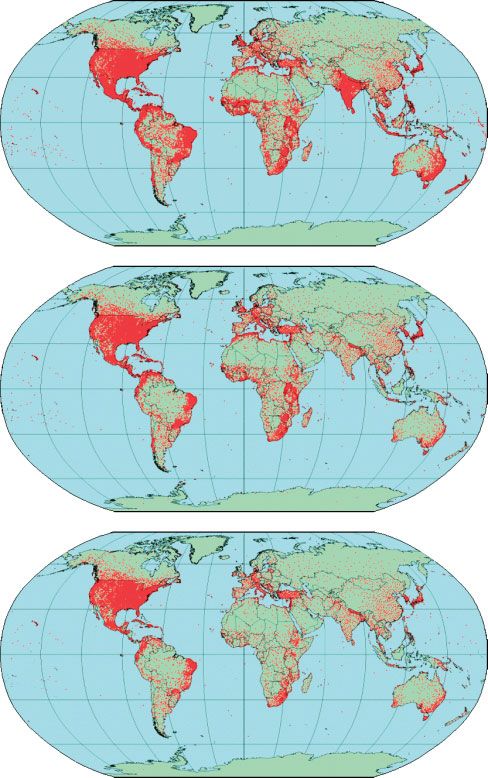
1966 R. J. HIJMANS ET AL.
States (http://www.daymet.org/; Thornton et al., 1997). The highest resolution interpolated climate database
for global land areas (excluding Antarctica) has a 10 arc min spatial resolution (18.5 km at the equator; New
et al., 2002). Leemans and Cramer (1991) and New et al. (1999) created important earlier data sets, at a
spatial resolution of 0.5° (55.6 km at the equator).
We compiled monthly averages of climate as measured at weather stations from a large number of global,
regional, national, and local sources, mostly for the 1950–2000 period. We interpolated these data using the
thin-plate smoothing spline algorithm implemented in ANUSPLIN (Hutchinson, 2004) and created global
(land areas only, excluding Antarctica) climate surfaces for monthly precipitation and minimum, mean, and
maximum temperature. Our surfaces have a 30 arc s spatial resolution; this is equivalent to about 0.86 km2
at the equator and less elsewhere and commonly referred to as ‘1-km’ resolution. The data are referred to as
the ‘WorldClim’ database and are available for download from http://www.worldclim.org.
Here, we describe the methods used to compile and interpolate the climate data. We present several analyses
to illustrate the uncertainty in both the input data and in the climate surfaces: we describe the elevation bias in
the weather stations, quantify within-grid cell variation in elevation, and analyze results from data partitioning
and cross validation. We aggregated the climate surfaces to a 10 arc min resolution to illustrate the benefits
of higher resolution surfaces and to compare our results to those of New et al. (2002). We also compared our
surfaces to two high-resolution data sets that cover the conterminous United States.
2. METHODS
2.1. Climate data compilation and processing
Weather station data were assembled from a large number of sources:
(1) The Global Historical Climate Network Dataset (GHCN) version 2. (http://www.ncdc.noaa.gov/pub/
data/ghcn/v2;Peterson and Vose, 1997). GHCN reports data by year and month, and we calculated monthly
means for the 1950–2000 period. GHCN has data for precipitation (20 590 stations), mean temperature
(7280 stations), and minimum and maximum temperature (4966 stations). For precipitation and mean
temperature, GHCN has global coverage, but there are large gaps in the geographic distribution of stations
with minimum and maximum temperature data. For some stations, “adjusted” data that had been through
homogeneity control procedures were used (Peterson and Easterling, 1994; Easterling and Peterson, 1995).
We included the adjusted data where available and used unadjusted data for the remainder of the stations.
(2) The WMO climatological normals (CLINO) for 1961–1990 (WMO, 1996). This database includes
monthly mean (3084 stations), minimum and maximum (both 2504 stations) temperature and precipitation
(4261 stations). WMO did extensive quality control on these data (WMO, 1996).
(3) The FAOCLIM 2.0 global climate database (FAO, 2001). This database contains monthly data. It has
precipitation data for 27 372 stations, mean temperature data for 20 825 stations, and minimum and
maximum temperature data for 11 543 stations. This database includes long-term averages (1960–1990)
as well as time series data for temperature and precipitation.
(4) A database assembled by Peter G. Jones and collaborators at the International Center for Tropical
Agriculture (CIAT) in Colombia. It includes mean monthly data for precipitation (18 895 stations), mean
temperature (13 842 stations), and minimum and maximum temperature (5321 stations). This database
has data for the (sub)tropics only and is particularly data rich for Latin America.
(5) Additional regional databases for Latin America and the Caribbean (R-Hydronet; http://www.r-hydronet.sr.
unh.edu/english/), the Altiplano in Peru and Bolivia (INTECSA, 1993), the ‘Nordic Countries’ in
Europe (Nordklim, http://www.smhi.se/hfa coord/nordklim/), Australia (BOM, 2003), New Zealand
(http://www.metservice.co.nz/), and Madagascar (database accompanying Oldeman, 1988).
The GHCN data set has undergone the most explicit quality control (Peterson et al., 1997). For this reason,
additional records from other databases were only added if they were further than 5 km away from stations
already in that database and were added in the order as listed above. In this way, most duplicate records
Copyright 2005 Royal Meteorological Society Int. J. Climatol. 25: 1965–1978 (2005)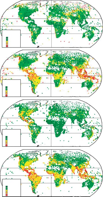
GLOBAL CLIMATE SURFACES 1967 among the different sources were removed (the same stations often appear in different databases with slightly different coordinates or names). Where the number of years that was used to calculate mean values for a record was known, we only added records with at least 10 years of data. We initially intended to include climate data for the 1960–1990 period only, but we expanded this to the 1950–2000 period as it became clear that this significantly increased the number of records for some areas. For example, there are few records after 1960 for the D.R. Congo (formerly Zaire), while many of the records for the Brazilian Amazon area are rather recent. In other cases, the data was available as averages only, sometimes for the 1960–1990 period and sometimes for a different, or unknown, time period. We added these records because our first concern was to create surfaces of high spatial fidelity, and we assumed that, for most locations, deviations from the true climate during the 1950–2000 period are more likely to arise owing to an insufficiently dense station network than to climate change during the twentieth century. For example, for Madagascar, we added 35 mean temperature stations and 88 minimum and maximum temperature stations for the 1931–1960 period. For the few Madagascan stations we had time series for, we did not observe significant climate change between 1930 and 1990. 2.2. Interpolation A number of different statistical approaches have been used to generate interpolated climate surfaces. Thornton et al. (1997) used a truncated Gaussian weighting filter in combination with spatially and temporally explicit empirically determined relationships of temperature and precipitation to elevation. Daly et al. (2002) used the PRISM method, which allows for incorporation of expert knowledge about the climate and can be particularly useful when data points are sparse. With this method, one can explicitly account for the effects of coastal influence, terrain barriers, temperature inversions, and other factors on spatial climate patterns. Other approaches include Inverse Distance Weighting and Kriging (see Hartkamp et al., 1999, for an overview). We used the ANUSPLIN software package version 4.3 (Hutchinson, 2004) that implements the thin-plate smoothing splines procedure described by Hutchinson (1995). We chose this method because it has been used in other global studies (New et al., 1999, 2002), performed well in comparative tests of multiple interpolation techniques (Hartkamp et al., 1999; Jarvis and Stuart, 2001), and because it is computationally efficient and easy to run. We used the ANUSPLIN-SPLINA program, which uses every station as a data point, rather than SPLINB, which uses a subset of stations. We fitted a second-order spline using latitude, longitude, and elevation as independent variables because this produced the lowest overall cross-validation errors as compared with some other settings (e.g. third-order spline, elevation as a covariate). We had many more data points than could be used in a single run of SPLINA (owing to computer memory constraints), and we therefore divided the world into 13 overlapping zones. To obtain smooth transitions between zones, each zone overlapped at least 15° into its neighboring zones; adjacent zones with sparse data had more overlap (up to 30° ). SPLINA fits a continuous surface to the points, but, as in regression, the surface does not necessarily go through every observed point. 2.3. Quality control As a first means of identifying errors in the location of the weather stations, all stations were checked for correspondence between the reported country and the country they mapped in and between the reported elevation and the elevation obtained from our elevation grid (see the following text). We mapped and checked all stations that had a large deviation between the reported elevation and that of the grid cell in which it mapped and its direct ‘neighborhood’ (the eight grid cells surrounding this grid cell). The neighborhood approach was used because a 100-m difference in elevation is negligible in mountainous areas such as the Andes, given the within- and between-grid cell variation, but large in relatively flat areas such as the Amazon. We checked the coordinates of outlying stations by searching for the station name in the Alexandria Digital Gazetteer (http://www.alexandria.ucsb.edu/gazetteer/). Unless the data of either the elevation or location could be corrected with a high degree of certainty, the stations with large elevational discrepancies were left out of the analysis. We ran SPLINA several times for each zone. The program produces a list of the stations with the largest root mean square residuals (i.e. the difference between the station data and the fitted climate surface). Initially, Copyright 2005 Royal Meteorological Society Int. J. Climatol. 25: 1965–1978 (2005)
1968 R. J. HIJMANS ET AL. very large residuals could be traced to simple typographical errors as well as clear geo-referencing or reported elevation errors, and we removed or corrected records with large and obvious errors. When the source of error was not clear but deviations were deemed extreme and unlikely, e.g. for being strongly asynchronous with neighboring stations, data were also removed. After making a change to the input data, SPLINA was run again. We also visually inspected the consistency of the resulting surfaces (see the following text). 2.4. Construction of the climate surfaces The spatially continuous surfaces created by SPLINA can be interrogated for any specific location and elevation within the specified domain of interpolation. We used the LAPGRID program to do this for an array (grid) of locations and elevations. We used elevation data from the Shuttle Radar Topography Mission (SRTM) which obtained elevation data on a near-global scale with a radar system that flew onboard a space shuttle. For most parts of the world, this data set provides a dramatic improvement in the availability of high-quality and high-resolution elevation data (Jarvis et al., 2004). We used the 3 arc s (∼90 m) spatial resolution ‘hole-filled’ SRTM data set that is available at http://srtm.csi.cgiar.org/. We aggregated these data to 30 arc s spatial resolu- tion using the median value. We used the GTOPO30 database (http://edcdaac.usgs.gov/gtopo30/gtopo30.asp) for the areas where there no SRTM data was available (i.e. north of 60 ° N). We created monthly surfaces for precipitation and minimum, maximum, and mean temperatures. Because we had many more records for mean temperature than for minimum and maximum temperature, we did the following to ensure that the surfaces were mutually consistent and used the available original data to the largest extent possible: for each month, surfaces of temperature range were calculated as the difference between those of interpolated maximum and minimum temperatures. The final surfaces of minimum and maximum temperatures were then calculated as the mean temperature surface minus or plus half the temperature range surface. We initially tried an alternative and more direct approach of interpolating temperature range but discontinued doing this because we found it much harder to check errors on the temperature range data than on the original minimum and maximum temperature data. The latitude/longitude geographical coordinate system was used for all climate surfaces. The upper left corner is at 180 ° W and 90 ° N, and the lower right corner is at 180 ° E and 60 ° S. This area includes all major landmasses except Antarctica. The surfaces consist of 43 200 columns and 18 000 rows, with a total of 7.8 × 10⁸ cells of which 28% designate land. All cells have a 30 arc s horizontal and vertical resolution. The size of a 30-s grid cell changes with latitude and is approximately 0.861 km2 at the equator. This area decreases further north or south, and this distorts the interpolation, but the expected error due to this distortion is small. 2.5. Uncertainty Uncertainty in climate surfaces stems from the quality of the input data and the interpolation method used. We illustrate the geographic variation in uncertainty by carrying out a number of complimentary analyses. We calculated elevation bias in weather stations as the difference between the mean elevation of a 2-degree grid cell and the mean elevation of the weather stations therein. Two-degree grid cells were used in order to have a large number of stations in most cells so that the results should become regionally coherent and not dominated by outliers. Within-grid cell variation in elevation was evaluated by mapping the range of elevations of the 3 arc s resolution grid cells within each 30 arc s cell. We also partitioned the stations into a test and training set, each containing a random set of half the stations. We then used SPLINA to build continuous climate surfaces for the training data and interrogated these surfaces for the locations of the test data. We mapped the mean differences between the observed and predicted climate on the 2-degree grid for precipitation and temperature (means across all months). In each interpolation, ANUSPLIN performs cross validation by holding out each station in turn and calculat- ing the difference between the observed and predicted values at that station’s location. We mapped the means of these cross-validation errors on the 2-degree grid for precipitation and temperature (means across all months). 2.6. Scale and comparison with earlier work To illustrate the importance of high-resolution climate surfaces, we calculated the within-cell range of elevation, mean annual temperature, and total annual precipitation for a 10 arc min resolution grid. This Copyright 2005 Royal Meteorological Society Int. J. Climatol. 25: 1965–1978 (2005)
GLOBAL CLIMATE SURFACES 1969
resolution was chosen because it is the highest resolution global climate data set that was available before our
study (New et al., 2002) and in order to compare with that data set. We aggregated our estimates of annual
mean temperature and annual precipitation to a 10 arc min resolution (calculating the mean values) to compare
these with the surfaces from New et al. (2002). We also compared mean temperature and annual precipitation
on our surfaces to two other sets of high-resolution climate surfaces for the conterminous United States: the 1-
km-resolution Daymet database of means for 1980–1997 (http://www.daymet.org/; Thornton et al., 1997) and
the 2.5 arc min (∼5 km) PRISM climate database for 1970–2000 (http://www.ocs.orst.edu/; Daly et al., 2002).
3. RESULTS
3.1. Data cleaning
We removed or corrected a large number of errors. Some of these were caused by obvious typos, clearly
wrong coordinates, or the use of different units like Fahrenheit versus Celsius, or feet versus meters. For
example, in the GHCN database, there were a number of records for India where altitude was expressed as
meters multiplied by 3.3; it appeared that data expressed in meters was erroneously assumed to be in feet
and was converted to meters. Another problem were the mix-up of extreme and mean monthly minimum and
maximum temperatures. For example, extreme, not mean, minimum and maximum monthly temperatures seem
to be included for Poland and the United Kingdom in the GHCN and other databases. In the case of Poland,
this problem was spotted because the resulting surfaces indicated unexpected low and high temperatures
almost exactly coinciding with the area of this country. Yet, these stations were not listed among the stations
with high residuals in SPLINA. It appears that the list of residuals is good for finding individual outliers
among relatively similar nearby stations. However, it is less adept at finding errors in cases where whole
groups of stations or geographically isolated stations are wrong; these errors can only be found through visual
inspection of the surfaces.
3.2. Distribution of weather stations
After removing stations with errors, our database consisted of precipitation records from 47 554 locations,
mean temperature from 24 542 locations, and minimum and maximum temperatures from 14 835 locations,
although some duplicate stations still remain (Figure 1). The geographic distribution of the stations is clearly
not random. There are few stations in areas with low population density such as the Arctics (including
Greenland), Siberia, the Amazon, Patagonia, Tibet, the Sahara, and other deserts. The distribution of stations
appears to be not only related to levels of economic development of a country but also to a combination
of investments in a meteorological observation network and national data access policies. For example,
climate data from the United States is generally easily accessible, unlike data from, e.g. many European
countries. Elevation bias in weather stations is related to latitude and, obviously, to the presence of mountains
(Figure 2(A)). In the tropics, stations tend to be biased toward higher elevations (particularly in Africa and
the Andes, but with the exception of parts of southeast Asia), and elsewhere they are biased toward low
elevations (particularly in the Himalayas and in parts of northwestern United States and Canada).
3.3. Uncertainty
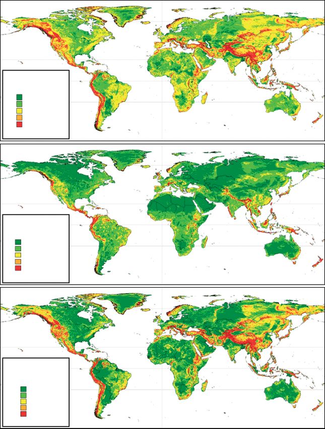
Variation of 3 arc s elevation data within 30 arc s grid cells is below 50 m in the vast majority of grid cells
(Figure 2(B)). Nevertheless, in major mountain ranges, within-grid cell variation can be 500 m and larger.
Data partitioning (Figure 3(A) and (C)) led, as expected when using only half the data in the prediction,
to much higher deviations from the observed data than cross validation (Figure 3(B) and (D)). Both
methods identified deviations of precipitation to be highest in areas with high precipitation, which is not
surprising. The cross-validation error is reasonably low at 50 mm/month) but not with cross validation indicates that the coverage of the stations network
might just be dense enough to provide a reasonable estimate with the stations available.
Temperature deviations tend to be very small in cross validation (Figure 3(C);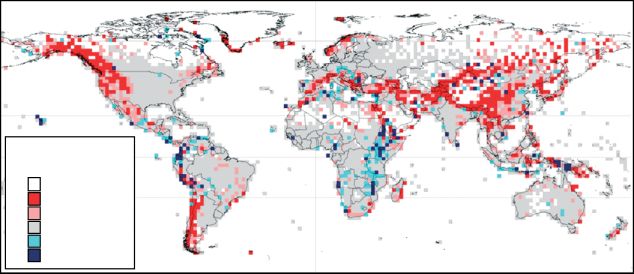
1970 R. J. HIJMANS ET AL.
A
B
C
Figure 1. Locations of weather stations from which data was used in the interpolations. (A) precipitation (47 554 stations); (B) mean
temperature (24 542 stations); (C) maximum or minimum temperature (14 930 stations). This figure is available in colour online at
www.interscience.wiley.com/ijoc
that there is much error in the station data for these areas. With partitioning, most areas have mean errors in
temperatures between 0 and 1 ° C (Figure 3(D)).
3.4. Resolution and comparison with previous studies
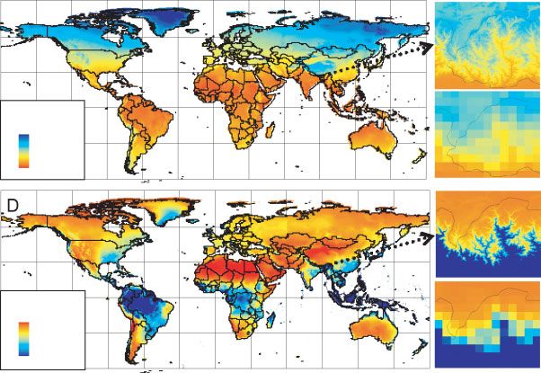
Our climate surfaces (Figure 4) reflect known patterns in global climate. One of the main differences
with previous studies is the high resolution of our data (Figure 4(B) and (E)). Variation within cells of a
10 arc min spatial resolution grid is very large (Table I), particularly in mountainous areas (Figure 5). The
Copyright 2005 Royal Meteorological Society Int. J. Climatol. 25: 1965–1978 (2005)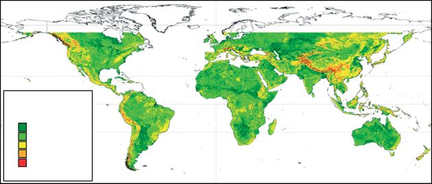
GLOBAL CLIMATE SURFACES 1971
(A)
Elevation bias (m)
No stations
< -250
-250 - -100
-100 - 100
100 - 250
> 250
(B)
Within grid cell variation
in elevation (m)
0 - 10
10 - 50
50 - 250
250 - 500
500 - 1905
Figure 2. (A) Elevation bias in rainfall stations, here defined as the mean elevation in a 2-degree grid cell minus that of the stations
in that cell. (B) The elevation range of 3 arc s (∼90 m) resolution elevation data within a 30 arc s (∼1 km) grid cell, for areas where
SRTM data is available. This figure is available in colour online at www.interscience.wiley.com/ijoc
upper quartiles of the within-grid cell ranges were considerable: 327 m (elevation), 85 mm (precipitation), and
2.5 ° C (temperature), but the maximum ranges are very large: 5068 m (elevation), 7925 mm (precipitation),
and 33.8 ° C (temperature) (Table I).
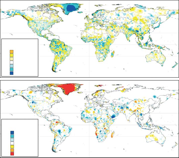
Despite the overall similarity in global climate patterns, the differences as compared to New et al. (2002)
can be large (Figure 6). Some of these differences can be attributed to differences in elevation data (e.g.
the Pantepui highlands in Venezuela and parts of the Andes in Peru for which the SRTM data is radically
different and much superior to previously available elevation data). Other differences are related to the use
of a different set of weather stations, and, no doubt, to some residual errors in our data set and that of New
et al. (2002). The differences in Greenland are extreme. There are only a few weather stations on the coast
of Greenland, and the predictions for the inland areas are clearly very speculative (Figures 1 and 6). The
methods of creating the 10 arc min surfaces were also different. Our method was a mean climate across the
30 arc s grid cells, whereas New et al.’s method was an estimate of the climate in the center of the 10 arc min
grid cell for the elevation of that cell.
Our surfaces were very similar to the Daymet and PRISM surfaces for the eastern United States. However,
there were large differences in the Rocky Mountains and in other mountainous areas further west. This is
illustrated in the maps of Figures 7 and 8 that cover the area with most variation, the states of Washington
and Oregon. Although the surfaces show similar regional trends, they also show strong disagreement about
local climates. Differences of 100 mm in precipitation were common, Daymet being overall much wetter than
Copyright 2005 Royal Meteorological Society Int. J. Climatol. 25: 1965–1978 (2005)1972 R. J. HIJMANS ET AL.
A
Mean Temperature-
Mean Partitioning
Difference (C)
0 - 0.5
0.5 - 1
1-2
2-3
>3
B
Precipitation-
Mean Partitioning
Difference (mm)
0-5
5 - 10
10 - 25
25 - 50
> 50
C
Mean Temperature-
Mean Cross-Validation
Difference (°C)
0 - 0.1
0.1 - 0.2
0.2 - 0.3
0.3 - 0.4
> 0.4
D
Precipitation-
Mean Cross-Validation
Difference (mm)
0-1
1-2
2-3
5 - 10
> 10
Figure 3. Uncertainty in the climate surfaces. Mean cross-validation deviations for precipitation (A) and mean temperature (C) and
deviations when partitioning data in test and training sets for precipitation (B) and mean temperature (D). Values are averaged across
12 months and by 2-degree grid cell. This figure is available in colour online at www.interscience.wiley.com/ijoc
WorldClim, and PRISM showing both much wetter and much drier areas than the other two. For temperature,
Daymet and WorldClim were very similar, but different from PRISM.
There were also considerable differences in the extreme values observed in the area mapped on Figures 7
and 8. Our annual precipitation surface had values between 165 and 3384 mm, but PRISM (149–6969) and
Copyright 2005 Royal Meteorological Society Int. J. Climatol. 25: 1965–1978 (2005)GLOBAL CLIMATE SURFACES 1973
(A)
(B)
(C)
Mean annual
temperature (°C)
-30.1
30.5
(D) (E)
(F)
Annual
precipitation (mm)
0
12084
Figure 4. Mean annual temperature (A) and annual precipitation (D). Close ups for an area including western Bhutan of about 220 by
190 km at the 30 arc s (∼1 km) resolution (B and E) and at a 10 arc min (∼18 km) resolution (C and F). This figure is available in
colour online at www.interscience.wiley.com/ijoc
Table I. Within-grid cell variation (minimum, lower quartile, mean, upper quartile, and maximum values) of 3 arc s
elevation data within grid cells of 0.5 arc min resolution; and, for elevation, annual precipitation, and mean annual
temperature, of 30 arc s grid cells within 10 and 30 min grid cells
Resolution Minimum Lower Mean Upper Maximum
(arc min) quartile quartile
Elevation (m) 0.5 0 25 67 76 1905
10 0 62 347 459 5068
30 0 135 621 878 7153
Precipitation (mm) 10 0 13 87 85 7925
30 0 33 184 191 8816
Temperature (° C) 10 0 0.3 1.8 2.5 33.8
30 0 0.8 3.3 4.6 44.6
Daymet (184–7148) had much higher maximum values. These high values occurred at high elevations, where
there are few, if any, weather stations. Our temperature surface had values between −9.8 and 16 ° C, which
was comparable to those of Daymet (−10.8 to 15.6 ° C), whereas the lowest temperature for PRISM was
−1.8 ° C. The stark difference in the lowest temperature observed is mostly related to resolution. The coldest
areas are on mountain peaks, which, because of their small spatial extent, are not represented on the coarser
spatial resolution PRISM data.
4. DISCUSSION
Our database has a 400 times higher spatial resolution than previously available surfaces (New et al., 2002);
it was derived from more weather stations (New et al. had 57% of our number of stations for precipitation,
Copyright 2005 Royal Meteorological Society Int. J. Climatol. 25: 1965–1978 (2005)1974 R. J. HIJMANS ET AL.
(A)
Elevation range (m)
0 - 25
25 - 100
100 - 500
500 - 1000
1000 - 5068
(B)
Precipitation range (mm)
0 - 25
25 - 100
100 - 250
250 - 500
500 - 7925
(C)
Temperature range (°C)
0 - 0.5
0.5 - 1
1 - 2.5
2.5 - 5
5 - 33.8
Figure 5. Within-grid cell variation (range of values) of (A) elevation, (B) annual precipitation, and (C) mean temperature of the
values on a 30 arc s (∼1 km) spatial resolution grid within a 10 arc min (∼18 km) grid. This figure is available in colour online at
www.interscience.wiley.com/ijoc
Copyright 2005 Royal Meteorological Society Int. J. Climatol. 25: 1965–1978 (2005)GLOBAL CLIMATE SURFACES 1975
Difference in precipitation
(mm)
< -500
-500 - -50
-50 - -10
-10 - 10
10 - 50
50 - 500
> 500
Difference in mean
temperature (°C)
< -2.0
-2 - -1
-1 - -0.5
-0.5 - 0.5
0.5 - 1
1-2
>2
Figure 6. Difference between our climate surfaces and those of New et al. (2002) for mean annual temperature and annual precipitation.
This figure is available in colour online at www.interscience.wiley.com/ijoc
52% for mean temperature, and 74% for temperature range), even when accounting for some duplicates in
our data set; and it benefited from a new and more accurate global elevation data set. New et al. (2002)
interpolated more climate elements (including, e.g. solar radiation and wind speed). In future work, we plan
to also include these additional climate elements and incorporate data from additional weather stations as
these become available.
Climate data at this very high resolution may be essential for studies in mountain environments and other
areas with strong climate gradients. The availability of these data allow for the evaluation of their utility with
respect to data at a lower spatial resolution. The effect of climate data resolution on modeling results is rarely
considered but can now be investigated across a wide range of spatial resolutions ≥1 km.
The high resolution of our surfaces does not imply that the quality of the data is necessarily high in all
places. The quality of the surfaces is spatially variable and depends on the local climate variability in an
area, the quality and density of the observations, and the degree to which a spline can be fitted through it.
Owing to the overall low density of available climate stations, and ignoring locally important drivers such as
aspect, our surfaces do not capture all the variation that may occur at a resolution of 1 km, particularly of
precipitation in mountainous areas.
Copyright 2005 Royal Meteorological Society Int. J. Climatol. 25: 1965–1978 (2005)1976 R. J. HIJMANS ET AL.
WorldClim PRISM Daymet
Annual precipitation (mm)
165 - 300
301 - 500
501 - 750
751 - 1000
1000 - 1500
1500 - 2000
2000 - 2500
2500 - 3500
3500 - 7148
PRISM - WorldClim Daymet - WorldClim Daymet - PRISM
Difference
< -500
-500 - -100
-100 - 100
100 - 500
> 500
0 km 300
Figure 7. Comparison of annual precipitation according to WorldClim with PRISM and Daymet, two high-resolution data sets for the
conterminous United States. We map the values and pairwise differences between these data sets for the states of Washington and
Oregon, an area where the differences were very large. This figure is available in colour online at www.interscience.wiley.com/ijoc
WorldClim PRISM Daymet
Mean temperature (°C)
< -2.5
-2.5 - 0
0 - 2.5
2.5 - 5
5 - 7.5
7.5 - 9
9 - 10.5
10.5 - 12.5
> 12.5
PRISM - WorldClim Daymet - WorldClim Daymet - PRISM
Difference
< -2.5
-2.5 - -1
-1 - -0.5
-0.5 - 0.5
0.5 - 1
1 - 2.5
> 2.5
0 km 300
Figure 8. Comparison of mean temperature according to WorldClim with PRISM and Daymet, two high-resolution data sets for
the conterminous United States. We map the values and pairwise differences between these data sets for the states of Washington
and Oregon, an area where the differences between the datasets were very large. This figure is available in colour online at
www.interscience.wiley.com/ijoc
Copyright 2005 Royal Meteorological Society Int. J. Climatol. 25: 1965–1978 (2005)GLOBAL CLIMATE SURFACES 1977 It is important to note that the climate models created by ANUSPLIN-SPLINA are continuous. The resolution of the data thus only depends on the grid that is used to sample the continuous prediction (with the ANUSPLIN-LAPGRD program), and the higher the resolution of the grid, the better it represents the modeled climate data. A high-resolution climate grid hides less of the spatial variation that is known to the model. This was illustrated by the high within-grid cell variation when aggregating our data to 10 arc min. We have provided a number of different analyses of data quality and uncertainty. Data partitioning and cross validation are excellent tools to compare between different interpolation methods, but are less useful when considering a single set of surfaces. A problem with these methods is that they can only evaluate the surfaces for places where there are stations. The largest geographically consistent differences between our results and those of New et al. (2002) were in areas of low station density, and station density may be the single best indicator of the reliability of the surfaces. Owing to the overall low density of the available climate stations, our surfaces do not capture of all variation that may occur at a spatial resolution of 1 km, particularly of precipitation in mountainous areas. Although there was overall agreement between three data sets of high-resolution surfaces for the eastern United States, differences in parts of the western mountainous areas were very large. This clearly indicates that we cannot be very certain about the values of any particular grid cell in these areas. The differences we found likely reflect the difference between a pure statistical and a more mechanistic expert-driven approach to interpolation. Model comparison work focusing on these geographic areas would be useful because in our comparison the effects of interpolation method are confounded with differences in resolution, climate and elevation data sources used, and the time period considered. Apart from areas with a low station density, the highest uncertainty in climate data is in areas with high variation in elevation. Elevation bias is clearly present in the stations network we used, but it is unclear how much, and where, this affects the results. Briggs and Cogley (1996) showed that in the United States weather stations tend to be biased toward lower elevations, and our results confirm this, but show that while this pattern is common at high latitudes and in the subtropics, it tends to be reversed in the tropics. The extent to which uncertainty in mountainous areas should be a problem depends on the application of the data. If climate-based predictions are made, and their success is measured in terms of the area correctly classified, the larger uncertainty in mountain areas may be completely offset by the stronger climate gradients; that is, a small error in a region with a shallow climate gradient can lead to an incorrect classification of a larger area compared to regions with a steep climate gradient. While there are a number of large global databases, many stations are not included in any of these. Moreover, the databases partly overlap and partly contradict each other. Studies like ours would therefore greatly benefit from expanding the number of stations for which data is readily available, particularly when this goes hand in hand with increased quality control. Projects like the GHCN (Peterson and Vose, 1997) are extremely important in this respect. Such projects should include efforts to reconcile the locality (coordinates) and elevation of the stations, and assess their spatial uncertainty (Wieczorek et al., 2004), as well as assign internationally useful station codes (WMO codes) so that different databases can be merged more easily. Apart from better and more input data, there are additional ways in which future research might improve our climate surfaces. For example, interpolations could be carried out on a regional scale and then merged into a global data set. To create our surfaces, we used a second-order spline and elevation as an independent variable because this gave the best overall fit (see Methods, data not shown). However, it might be that in some regions of the world, alternative settings (e.g. third-order spline, elevation as a covariate) would fit the data better. If regional interpolations are done in collaboration with climatologists familiar with the area, and within a knowledge-based framework, much more of the known regional climatic peculiarities might be captured. Such an approach could also investigate the value of correcting, or removing, data from time periods other than the one being considered. We did not remove such data because we think that this improved the overall quality of our data, but in areas with notable levels of climate change during the twentieth century, this may not be justified. Additional independent variables could also be included (Jarvis and Stuart, 2001). Remotely sensed data could be particularly useful to obtain more certainty about the climate for remote places such as Greenland, the Sahara desert, and the Amazon. Yet, insufficient high-resolution long-term global satellite data has been assembled to date. Copyright 2005 Royal Meteorological Society Int. J. Climatol. 25: 1965–1978 (2005)
1978 R. J. HIJMANS ET AL.
In conclusion, while we have made significant progress, additional efforts to compile and capture climate
data are needed to improve spatial and temporal coverage of the available climate data and quality control
(Mitchell and Jones, 2005), and interpolation methods can be further refined to better use these data. Evaluation
of the sources and amounts of uncertainty, and comparisons between data sets, as was done in this study,
provide both insight into the geographic distribution of uncertainty as well as a starting point for improvement
of the surfaces that is targeted at the areas where this may impact the results most.
ACKNOWLEDGEMENTS
The study was partly funded by NatureServe. SEC was funded by a National Science Foundation Graduate
Research Fellowship. We thank Simon Ferrier, Catherine Graham, Craig Moritz, and Karen Richardson for
encouragement; David Lees for sharing data; and Michael Hutchinson for advice.
REFERENCES
BOM. 2003. The Australian Data Archive of Meteorology. Bureau of Meteorology, Commonwealth of Australia: Melbourne, Australia.
Briggs PR, Cogley JG. 1996. Topographic bias in mesoscale precipitation networks. Journal of Climate 9: 205–218.
Daly C, Gibson WP, Taylor GH, Johnson GL, Pasteris P. 2002. A knowledge-based approach to the statistical mapping of climate.
Climate Research 22: 99–113.
Easterling DR, Peterson TC. 1995. A new method for detecting and adjusting for undocumented discontinuities in climatological time
series. International Journal of Climatology 15: 369–377.
FAO. 2001. FAOCLIM 2.0 A World-Wide Agroclimatic Database. Food and Agriculture Organization of the United Nations: Rome, Italy.
Hartkamp AD, De Beurs K, Stein A, White JW. 1999. Interpolation Techniques for Climate Variables, NRG-GIS Series 99-01. CIMMYT:
Mexico, DF, http://www.cimmyt.org/Research/nrg/pdf/NRGGIS%2099 01.pdf [1 Sep 2004].
Hijmans RJ, Condori B, Carillo R, Kropff MJ. 2003. A quantitative and constraint-specific method to assess the potential impact of
new agricultural technology: the case of frost resistant potato for the Altiplano (Peru and Bolivia). Agricultural Systems 76: 895–911.
Hutchinson MF. 1995. Interpolating mean rainfall using thin plate smoothing splines. International Journal of Geographical Information
Systems 9: 385–403.
Hutchinson MF. 2004. Anusplin Version 4.3. Centre for Resource and Environmental Studies. The Australian National University:
Canberra, Australia.
Jarvis CH, Stuart N. 2001. A comparison among strategies for interpolating maximum and minimum daily air temperatures. Part II:
the interaction between the number of guiding variables and the type of interpolation method. Journal of Applied Meteorology 40:
1075–1084.
Jarvis A, Rubiano J, Nelson A, Farrow A, Mulligan M. 2004. Practical Use of SRTM Data in the Tropics: Comparisons with Digital
Elevation Models Generated from Cartographic Data. Working Document 198. International Center for Tropical Agriculture: Cali,
Colombia.
Jones PG, Gladkov A. 2003. FloraMap. A Computer Tool for Predicting the Distribution of Plants and Other Organisms in the Wild.
Version 1.02. Centro Internacional de Agricultura Tropical: Cali, Colombia.
Leemans R, Cramer WP. 1991. The IIASA Database for mean Monthly Values of Temperature, Precipitation and Cloudiness of a Global
Terrestrial Grid . Research Report RR-91-18 November 1991. International Institute of Applied Systems Analyses: Laxenburg, Austria.
INTECSA. 1993. Estudio de Climatologı́a. Plan director Global Binacional de Protección – Prevención de Inundaciones y
Aprovechamiento de Los Recursos del Lago Titicaca, rı́o Desaguadero, Lago Poopó y Lago Salar de Coipasa (Sistema T.D.P.S).
INTECSA, AIC, CNR: La Paz, Bolivia.
Mitchell TD, Jones PD. 2005. An improved method of constructing a database of monthly climate observations and associated high-
resolution grids. International Journal of Climatology 25: 693–712.
New M, Hulme M, Jones P. 1999. Representing twentieth-century space-time climate varibility. Part I: Development of a 1961–90
mean monthly terrestial climatology. Journal of Climate 12: 829–856.
New M, Lister D, Hulme M, Makin I. 2002. A high-resolution data set of surface climate over global land areas. Climate Research 21:
1–25.
Oldeman LR. 1988. An Agroclimatic Characterization of Madagascar. International Soil Reference and Information Centre: Wageningen,
Netherlands.
Parra JL, Graham CC, Freile JF. 2004. Evaluating alternative data sets for ecological niche models of birds in the Andes. Ecography
27: 350–360.
Peterson TC, Easterling DR. 1994. Creation of homogenous composite climatological reference series. International Journal of
Climatology 14: 671–679.
Peterson TC, Vose RS. 1997. An overview of the Global Historical Climatology Network temperature data base. Bulletin of the American
Meteorological Society 78: 2837–2849.
Peterson TC, Vose R, Schmoyer R, Razuvaev V. 1997. Global Historical Climatology Network (GHCN) quality control of monthly
temperature data. International Journal of Climatology 18: 1169–1180.
Thornton PE, Running SW, White MA. 1997. Generating surfaces of daily meteorology variables over large regions of complex terrain.
Journal of Hydrology 190: 214–251.
Wieczorek JR, Guo Q, Hijmans RJ. 2004. The point-radius method for georeferencing point localities and calculating associated
uncertainty. International Journal of Geographical Information Science 18: 745–767.
WMO. 1996. Climatological Normals (CLINO) for the period 1961–1990. World Meteorological Organization: Geneva, Switzerland.
Copyright 2005 Royal Meteorological Society Int. J. Climatol. 25: 1965–1978 (2005)You can also read