A Synthesizing Land-cover Classification Method Based on Google Earth Engine: A Case Study in Nzhelele and Levhuvu Catchments, South Africa ...
←
→
Page content transcription
If your browser does not render page correctly, please read the page content below
Chin. Geogra. Sci. 2020 Vol. 30 No. 3 pp. 397–409                                                  Springer           Science Press
https://doi.org/10.1007/s11769-020-1119-y                                                   www.springerlink.com/content/1002-0063

A Synthesizing Land-cover Classification Method Based on Google
Earth Engine: A Case Study in Nzhelele and Levhuvu Catchments,
South Africa

ZENG Hongwei1, 2, WU Bingfang1, 2, WANG Shuai3, MUSAKWA Walter4, TIAN Fuyou1, 2, MASHIMBYE Zama
Eric5, POONA Nitesh5, SYNDEY Mavengahama6
(1. State Key Laboratory of Remote Sensing Science, Aerospace Information Research Institute, Chinese Academy of Sciences, Beijing
100101, China; 2. University of Chinese Academy of Sciences, Beijing 100049, China; 3. State Key Laboratory of Earth Surface Proc-
esses and Resource Ecology, Faculty of Geographical Science, Beijing Normal University, Beijing 100875, China; 4. Department of
Town and Regional Planning, University of Johannesburg, Johannesburg 2028, South Africa; 5. Department of Geography and Envi-
ronmental Studies, Stellenbosch University, Stellenbosch 7600, South Africa; 6. Department of Crop Science, Faculty of Natural and
Agricultural Sciences, North West University, Mmabatho 2745, South Africa)

Abstract: This study designed an approach to derive land-cover in the South Africa with insufficient ground samples, and made a case
demonstration in Nzhelele and Levhuvu catchments, South Africa. The method was developed based on an integration of Landsat 8,
Sentinel-1, and Shuttle Radar Topography Mission (SRTM) Digital Elevation Model (DEM), and the Google Earth Engine (GEE) plat-
form. Random forest classifier with 300 trees is employed as land-cover classification model. In order to overcome the defect of insuffi-
cient ground data, the stratified sampling method was used to generate the training and validation samples from the existing land-cover
product. Likewise, in order to recognize different land-cover categories, the percentile and monthly median composites were employed
to expand input metrics of random forest classifier. Results showed that the overall accuracy of the land-cover of Nzhelele and Levhuvu
catchments, South Africa in 2017–2018 reached to 76.43%. Three important results can be drawn from our research. 1) The participation
of Sentinel-1 data can slightly improve overall accuracy of land-cover while its contribution on land-cover classification varied with
land types. 2) Under-fitting problem was observed in the training of non-dominant land-cover categories using the random sampling, the
stratified sampling method is recommended to make sure the classification accuracy of non-dominant classes. 3) When related reflec-
tance bands participated in the training process, individual Normalized Difference Vegetation index (NDVI), Enhanced Vegetation Index
(EVI), Soil Adjusted Vegetation Index (SAVI), Normalized Difference Built-up Index (NDBI) have little effect on final land-cover clas-
sification result.
Keywords: land-cover classification; random forest; percentile composite; Landsat 8; Sentinel-1; Google Earth Engine (GEE)

Citation: ZENG Hongwei, WU Bingfang, WANG Shuai, MUSAKWA Walter, TIAN Fuyou, MASHIMBYE Zama Eric, POONA
Nitesh, SYNDEY Mavengahama, 2020. A Synthesizing Land-cover Classification Method Based on Google Earth Engine: A Case
Study in Nzhelele and Levhuvu Catchments, South Africa. Chinese Geographical Science, 30(3): 397–409. https://doi.org/10.1007/
s11769-020-1119-y

Received date: 2019-04-22; accepted date: 2019-09-04
Foundation item: Under the auspices of National Natural Science Foundation of China (No. 4171101213, 41561144013, 41991232),
  National Key R&D Program of China (No. 2016YFC0503401, 2016YFA0600304), International Partnership Program of Chinese
  Academy of Sciences (No. 121311KYSB20170004)
Corresponding author: WU Bingfang. E-mail: wubf@radi.ac.cn
© Science Press, Northeast Institute of Geography and Agroecology, CAS and Springer-Verlag GmbH Germany, part of Springer Na-
  ture 2020
398                                     Chinese Geographical Science 2020 Vol. 30 No. 3

1     Introduction                                                indices, and classification algorithms provide an effec-
                                                                  tive way for land-cover classification. For examples,
Land-cover product offer valuable information on the              recently, the latest finer resolution observation and
state of land surface, and it is requirement for the com-         monitoring of global land-cover with 10 m (FROM-
plex interactions between human activities, ecosystem,            GLC10) product was generated by random forest classi-
hydrologic, and global change (Running et al., 2008;              fier through using reflectance bands of Sentinel-2 and
Gong et al., 2013). As the development of satellite re-           series indicators (such as NDVI, MNDWI, NDBI and
mote sensing and classification algorithms improved, a            NBR) (Gong et al., 2019).
series of different land-cover products with different               With the emergence of new satellite sensors, the
spatial resolutions were generated in the past decades,           resolution and data volume has been increased greatly.
such as the global land-cover from 1km Moderate                   Great demands on computing capacity are required to
Resolution Imaging Spectroradiometer (MODIS) (Friedl              deal with multi-source satellite data. In the past few
et al., 2002), the global land-cover from Medium Reso-            years, the development of cloud computing, such as
lution Imaging Spectrometer (MERIS) fine resolution               Google Earth Engine (GEE) (Gorelick et al., 2017) may
(300 m) data (Arino et al., 2007), the Finer Resolution           provide a feasible way to overcome these challenges.
(30 m) Observation and Monitoring of Global Land-                 GEE platform powered by Google’s cloud infrastructure
cover (FROM-CLC30) from Landsat Thematic Mapper                   is designed as a planetary-scale platform for earth sci-
(TM) and Enhanced Thematic Mapper Plus (ETM+)                     ence data processing and analysis (Gorelick et al.,
data (Gong et al., 2013), the 30 m Globaland30 from               2017). GEE provides abundant earth observation data
Landsat TM, ETM+ and Huanjing-1 (HJ-1) (Chen et al.,              (such as MODIS, Landsat, and Sentinel satellite data). It
2015), and the Finer Resolution (10 m) Observation and            also freely provides a rich internet application pro-
Monitoring of Global Land-cover (FROM-GLC10)                      gramming interface and thousands of computers re-
from 10m Sentinel-2 data (Gong et al., 2019).                     sources for users. GEE provides multi ‘reducers’ and
   Obtaining land-cover products from remote sensing is           rich classifiers for land-cover classification (Zhang et
highly depended on the development and selection of               al., 2018; Gong et al., 2019; Singha et al., 2019; Tian et
classification algorithm and features extracted from the          al., 2019). Any user can easily access this huge data and
satellite data. For instance, classification algorithms for       carry out data processing and analysis through simple
the simple statistical classifiers (e.g., the maximum like-       script programming. Currently, GEE is widely used in
lihood classifier), classification trees (e.g., the classifi-     special class and general class classification, such as
cation and regression tree), and machine learning classi-         crop extent (Xiong et al., 2017), paddy rice (Dong et al.,
fiers (e.g., random forest and support vector machines)           2016; Zhang et al., 2018), maize (Tian et al., 2019),
were widely used for single, multi-temporal and                   mangrove forest map (Chen et al., 2017), and land-cover
multi-sources satellite imagery, respectively (Gong et            mapping (Gong et al., 2019).
al., 2013). For the features selection, many spectral in-            However, some issues of land-cover classification are
dicators were employed for special class information              not well addressed in the previous studies. In general,
extraction, such as Normalized Difference Vegetation              land types including shrub, grassland, and cropland
Index (NDVI) (Tucker, 1979), Enhanced Vegetation                  mixed regions are poorly identified (Gong et al., 2013).
Index (EVI) (Liu and Huete, 1995), and Soil Adjusted              For examples, the user accuracy of grasslands and shrub
Vegetation Index (SAVI) (Huete, 1988) for vegetation,             of the FROM-GLC 30 products was only 38.13% and
Normalized Difference Water Index (NDWI) (McFeet-                 39.04%, and their producer accuracy was only 29.40%
ers, 1996) and Modified Normalized Difference Water               and 34.00% for the random forest classifier (Gong et al.,
Index (MNDWI) (Xu, 2006) for open water surface,                  2013). The accuracy of shrub cover and grassland were
Normalized Difference Built-up Index (NDBI) (Zha et               still very poor in Africa even though stacked auto en-
al., 2003) and Index-based Built-up Index (IBI) (Xu,              coder-based deep learning classifier was used, the user
2008) for urban built-up areas, Normalized Burn Ratio             accuracy of shrub cover and grassland were 57.85% and
(NBR) (Miller and Thode, 2007) for burnt areas. The               45.42% and their producer accuracy were only 66.82%
combination of reflectance bands of sensors, spectral             and 38.48% (Li et al., 2016). Second, most land-cover
ZENG Hongwei et al. A Synthesizing Land-cover Classification Method Based on Google Earth Engine: A Case… 399
products were developed based on optical data, while ous southwest areas to 188 m in the northeast part. The
the contribution of synthetic aperture radar (SAR) is few precipitation is seasonal and generally occurs summer
explored in previous studies. Finally, although the fea- month from October to March (Makungo et al., 2010).
tures of the reflectance of sensor and indices can be ex- According to Climate Hazards Group InfraRed Precipi-
plored by monthly, percentile composite approaches and tation with Station data (CHIRPS) (Funk et al., 2015),
machine learning algorithm, the performance of the dif- Mean Annual Precipitation (MAP) from 1981 to 2016
ferent indices in the land-cover classification are under- was 554 mm for the whole region and varies from 1455
studied. Finally, how to effectively collect ground sam- mm in the southwest to 269 mm in north and northeast
ples are very important to the training of classifier and part. MAP varies monthly, with more than 80% precipi-
validation of land-cover classification result, while it is tation being dropped in the rainy season from October to
not easy to collect sample from the remote or undevel- March, and less than 20% precipitation in the dry season
oped regions. from April to September.
In this study, a synthesizing land-cover classification The land type of study site mainly includes forest,
method was developed to obtain land-cover of the shrub, grassland, cropland, and settlement. The land-
Nzhelele and Levuvhu catchments in South Africa with cover classification in this study is a big challenge due
insufficient ground samples. The study aims at answering to large proportion of tree cover and shrub cover. In the
the following three questions in somehow: 1) is SAR data last decades, land-cover types of this study site have
capable of improving the performance of land-cover clas- changed profoundly due to intensive human activities.
sification in shrubs, grassland, and sparse vegetation However, the change process is not well documented
mixed region; 2) which indices are sensitive to the due to the lack of land-cover product thereby hampering
land-cover classification; and 3) samples sampling how to comprehension of the coupled human and nature proc-
impact the classification performance. We hope the pro- ess.
posed approach can provides an alternative land-cover
classification choice for ground samples scarce areas in 2.2 Data and processing
the world, and improve their ability to mitigate climate 2.2.1 Remote sensing data and processing
change and promote sustainable development. (1) Landsat 8 OLI data
In order to cover the whole rainy and dry season, a total
2 Materials and Methods of 81 Landsat 8 Operational Land Imager (OLI) be-
tween October 2017 and September 2018 with atmos-
2.1 Study area pherically corrected surface reflectance were collected
Nzhelele and Levhuvu catchments are located in Lim- in this study. The number of images with cloud cover
popo Province of South Africa (29.70°E–31.40°E, percentage of 0–20%, 20%–40%, 40%–60%,
22.29°S–23.30°S), covering an area of 10 092 km2 (Fig. 1). 60%–80%, and 80%–100% are 38, 7, 10, 15, and 11
The elevation decreases from 1701 m in the mountain- respectively. The blue, green, red, Near Infrared (NIR),
Fig. 1 Geographical location of the Nzhele and Levhuvu catchments in South Africa400 Chinese Geographical Science 2020 Vol. 30 No. 3 Shortwave Infrared1 (SWIR1), and Shortwave Infrared collect the training and validation samples. The steps of 2 (SWIR2) bands were extracted and grouped as the samples extraction include: input features of classifier. More cropland samples were collected from the 30-m (2) Sentinel-1 GRD Global Food Security-support Analysis Data (GFSAD) SAR is sensitive to water, urban built, wetland, and cropland extent (Xiong et al., 2017). This product was paddy that indicates the using of SAR images may im- produced by automated cropland mapping using the prove the classification accuracy of land-cover. In this Google Earth Engine cloud computing with a weighted study, a total of 133 Sentinel-1 Ground Range Detected over all accuracy of 94%. Samples of forest type were (GRD) scenes with 10 m resolution were acquired for extracted from the 30-m Hansen Global Forest Change the period between October 2017 and September 2018. v1.6 (Hansen et al., 2013), this product is the result from Sentinel-1 GRD is the C-band synthetic aperture radar time-series analysis of Landsat images. Built-up areas data and it has Horizontal transmit/Horizontal receive samples were extracted from the 38-m Global Human (HH), Horizontal transmit/Vertical receive (HV), Verti- Settlement Layers (GHSL), built-up grid 2015(Pesaresi cal transmit/ Vertical receive (VV), Vertical trans- et al., 2016). This product was produced by Landsat 8 mit/Horizontal receive (VH) and angle bands. Each collection data from 2013 to 2014, census data, and Sentinel-1 scene in GEE data catalog was pre-processed crowd sources or volunteered geographic information with Sentinel-1 toolbox based on the following steps: sources. Samples of trees cover, shrubs cover, grassland, thermal noise removal, radiometric calibration, terrain cropland, vegetation aquatic, sparse vegetation, bare correction using DEM. The final terrain corrected values areas, built-up areas, and open water were collected are converted to decibels via log scaling (10 × log10x). from the S2 prototype LC that was generated by climate Detail is included on the website https://developers. change initiative land-cover team using the random for- google.com/earth-engine/sentinel1. The savitzky-golay est and machine learning based on 1 year of Sentinel-2A filter (Savitzky and Golay, 1964) was employed to filter observations between December 2015 and December the backscatter time series to minimize the influence of 2016. Samples of plantation were collected from the environmental conditions and to remove noises existing artificial visual interpretation. Plantation is an important in the Sentinel-1 datasets due to speckle. man-made land-cover in study area, the identification of 2.2.2 Topographic data it can assist in understanding the anthropogenic driving Elevation and slope can provide meaningful data for forces. Based on the field trip experience on July 2018 land-cover identification. SRTM global data with 30m and the knowledge of the local experts, this study used spatial resolution was collected in this study. It was the artificial visual interpretation to outline the ap- generated by interferometric radar data from dual radar proximate distribution of plantations. antenna and can be easily access from GEE earth cata- In order to ensure the quality of training and valida- log through script programming. In this study, its eleva- tion samples, this study used the following rules to re- tion and derived variable (slope) was taken as features fine forest, cropland and built-up areas products: 1) for- of the classifier for land-cover identification. est: the pixels are tree cover in S2 prototype LC and its 2.2.3 Data for training and validation samples forest coverage is above 40% in 30-m Hansen Global On July 2018, only 129 samples were collected from a Forest Change v1.6; 2) cropland: the pixels are identi- field trip, which the categories and number of these fied as cropland in 30-m cropland extent map of conti- samples are insufficient to train the classifier and vali- nental Africa and S2 prototype LC; 3) built-up areas: the date the classification result. To solve this issue of insuf- pixels are identified as settlement in 38-m global human ficient ground samples, some studies extracted samples settlement layers in 2015, and S2 prototype LC. from the existing land-cover products. For example, global forest change dataset (Hansen et al., 2013) and 2.3 Methods global water surface dataset (Pekel et al., 2016) were 2.3.1 Land-cover classification used in the identification of paddy (Zhang et al., 2018) This study adopted the land-cover classification system and maize (Tian et al., 2019). Under the inspiration of of European Space Agency (ESA) climate change initia- the above research, this study used the similar way to tive S2 prototype land-cover 20 map of Africa 2016
ZENG Hongwei et al. A Synthesizing Land-cover Classification Method Based on Google Earth Engine: A Case…      401

(hereinafter referred to S2 prototype LC), and the detail         ites for Landsat 8 OLI bands and indices and monthly
is included on the website http://2016africalandcover             median composite for Sentinel-1 GRD were adopted in
20m.esrin.esa.int/. The categories of S2 prototype LC in          this study. The training and validation samples were
Nzhele and Levhuvu catchments include trees cover,                extracted from S2 prototype LC, GHSL, Hansen Global
shrubs cover, vegetation aquatic, sparse vegetation, bare         Forest Change (Hansen et al., 2013), GFSAD cropland
areas, grassland, cropland, built-up areas, and water             extent (Xiong et al., 2017) and plantation extent from
surface. In July 2018, we organized a land-cover survey           artificial visual interpretation by stratified sampling ap-
in Nzhele and Levhuvu catchments and found that plan-             proach in GEE. A random forest classifier was em-
tation is an important type of land-cover in study site.          ployed to generate the land-cover product. Finally, the
Therefore, we added the plantation to S2 prototype LC             confusion matrix was used to assess the accuracy of
classification system and the updated classification sys-         land-cover classification result.
tem includes trees cover, shrubs cover, vegetation                2.3.2 Spectral indices
aquatic, sparse vegetation, bare areas, grassland, crop-          Vegetation types in Nzhelele and Levhuvu are diverse,
land, built-up areas, and water surface.                          covering the tree, sparse vegetation, shrub, and crop-
   Fig. 2 shows the classification flowchart. The input           land. In order to improve the distinction of vegetation
features of the random forest include the reflectance of          classes, Normalized Difference Vegetation Index
Blue, Green, Red, Near Infrared (NIR), Shortwave In-              (NDVI) (Tucker, 1979), Enhanced Vegetation Index
frared 1 (SWIR1), Shortwave Infrared 2 (SWIR2) of                 (EVI) (Huete et al., 2002), and Soil Adjusted Vegetation
Landsat 8 OIL images and their corresponding spectral             Index (SAVI) (Huete, 1988) were used in the classifier.
indices of NDVI, EVI, SAVI, NDWI and NDBI, VV                     These vegetation indices have been widely used for
and VH bands of Sentinel-1 GRD, and the elevation and             charactering growth status of vegetation. For instance,
slope from SRTM. In order to ensure temporary and                 NDVI is sensitive to chlorophyll absorption and it is
spectral information of these bands and indices can be            widely used to identify vegetation. EVI is a useful
adequately trained in the classifier, percentile compos-          vegetation index to enhance the vegetation signal with

Fig. 2   Overview of the methodology for land-cover mapping in Nzhelele and Levhuvu catchments, South Africa
402 Chinese Geographical Science 2020 Vol. 30 No. 3
an improved sensitivity to soil brightness (Huete et al., the rainy season from October to March in the next year.
1997). SAVI can highlight vegetation features in the There were about 36% of the Landsat 8 images with
area with low vegetation cover (Xu, 2008) and work cloud cover percentage higher than 40%. In this work,
well with vegetation cover as low as 15%. In addition, the percentile approach and monthly median composite
Normalized Difference Water Index (NDWI) (McFeet- were employed to conduct metric composites. The per-
ers, 1996) and the Normalized Difference Built-up In- centile approach in GEE can fully capture the spectrum
dex (NDBI) (Zha et al., 2003) are used to distinguish of Landsat 8 and nature vegetation phonological infor-
water surface and built-up areas of study area. These mation and widely used in the crop type mapping
indices were defined in Eqs. (1)–(5). (Zhang et al., 2018, Tian et al., 2019) and the land-cover
classification (Gong et al., 2019). For each input optical
NIR Red
NDVI = (1) feature collection, percentile approach will construct the
NIR + Red
histogram of feature collection and then calculate the
2.5 NIR Red specified percentiles of the feature distribution. Take the
EVI (2) reflectance of the blue band collection as one example,
NIR + 6 Red 7.5 Blue + 1
five metrics named ‘Blue_p5’, ‘Blue_p25’, ‘Blue_p50’,
NIR Red 1+ L ‘Blue_p75’, and‘Blue_p95’ would be generated when
SAVI = (3)
NIR + Red + L given 5, 25, 50, 75, and 95 in percentile composite. In
this study, percentiles’ percentage parameter are set to 5,
Green NIR 25, 50, 75 and 95 in percentile approaches, and then
NDWI (4)
Green NIR computed for all selected six reflectance bands collec-
tion and five indices collection of Landsat 8 OLI. A total
MIR NIR
NDBI (5) of 55 metrics were finally generated from selected re-
MIR NIR
flectance and spectral indices of Landsat 8 in GEE. This
where ρNIR, ρRed, ρBlue, ρGreen, ρMIR are surface reflectance study grouped all processed Sentinel-1 GRD images
acquired in the near-infrared, red, blue, green, and between October 2017 and September 2018 into
shortwave. L is the correction factor and is set to 0.5 in monthly images, and using the median composite to
this study. generate 24 metrics with 10 m resolution by monthly
2.3.3 Features composite approaches median composites, including 12 VH and 12 VV met-
It was difficult to composite 30-m resolution cloud free rics, respectively. A total of 79 metrics generated by
Landsat 8 images for each month as the quality of opti- percentile and monthly median composites are showing
cal data is seriously affected by the cloud, especially for in Table 1.
Table 1 Metrics generated by percentile approach and monthly median composites
Feature collection Name of metrics Composite method
Blue Blue_p5, Blue_p25, Blue_p50, Blue_p75, Blue_p95 Percentile composite
Green Green_p5, Green_p25, Green_p50, Green_p75, Green_p95
Red Red_p5, Red_p25, Red_p50, Red_p75, Red_p95
NIR NIR_p5, NIR_p25, NIR_p50, NIR_p75, NIR_p95
SWIR1 SWIR1_p5, SWIR1_p25, SWIR1_p50, SWIR1_p75, SWIR1_p95
SWIR2 SWIR2_p5, SWIR2_p25, SWIR2_p50, SWIR2_p75, SWIR2_p95
NDVI NDVI_p5, NDVI_p25, NDVI_p50, NDVI_p75, NDVI_p95
EVI EVI_p5, EVI_p25, EVI_p50, EVI_p75, EVI_p95
SAVI SAVI_p5, SAVI_p25, SAVI_p50, SAVI_p75, SAVI_p95
NDWI NDWI_p5, NDWI_p25, NDWI_p50, NDWI_p75, NDWI_p95
NDBI NDBI_p5, NDBI_p25, NDBI_p50, NDBI_p75, NDBI_p95
VV VVMON10,VVMON11,VVMON12,VVMON1,VVMON2,VVMON3,VVMON4,VVMON5,VVMON6,VVM Monthly median composite
ON7,VVMON8,VVMON9
VH VHMON10,VHMON11,VHMON12,VHMON1,VHMON2,VHMON3,VHMON4,VHMON5,VHMON6,VHM
ON7,VHMON8,VHMON9ZENG Hongwei et al. A Synthesizing Land-cover Classification Method Based on Google Earth Engine: A Case… 403
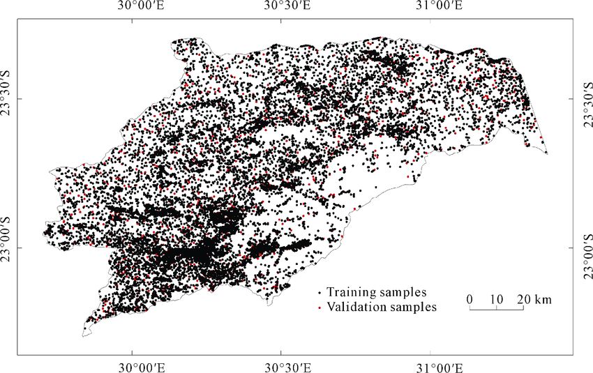
2.3.4 Training and validation samples generation 2.3.6 Accuracy assessment
methods Confusion matrix is used for accuracy assessment of
The result of land-cover classification is sensitive to the each land-cover type. The indicators of User Accuracies
number and distribution of samples. The missing or im- (UA), Producer Accuracies (PA), and the Overall Accu-
balance of training samples has the negative impact on racy (OA) are calculated as follows:
the parameter of classifier. The stratified sampling X ij
method in GEE can extract the same quantity samples UA = 100% (6)
Xj
for each class and can avoid over-fitting or un-
der-fitting phenomena. Based on this method, a total of X ij
19 249 training samples and 8154 validation samples PA = 100% (7)
Xi
were generated by stratified sampling approach in GEE
(Fig. 3). sd
OA = 100% (8)
2.3.5 Classifier: random forest n
The random forest classifier uses tree bagging to form
where Sd represents the total number of correctly classi-
an ensemble of trees by searching random subspaces in
fied pixels, n represents the total number of validation
the given features, then splitting the nodes by minimiz- pixels, and Xij represents an observation in row i and
ing the correlation between the trees (Breiman, 2001). column j in the confusion matrix; Xi represents the mar-
Random forest classifier has been widely used in ginal total of row i, and Xj represents the marginal total
land-cover mapping (Yu et al., 2014; Wang et al., 2015; of column j in the confusion table.
Gong et al., 2019) and crop type identification (Zhang et
al., 2018; Singha et al., 2019; Tian et al., 2019). Studies 3 Results
indicated that random forest has its merit for robustness,
high efficiency and high accuracy outcome in process- 3.1 Land-cover classification result
ing high dimensional data (Breiman, 2001), so that ran- The land-cover map in 2017–2018 based on classifica-
dom forest classifier was employed to conduct tion approaches was shown in Fig. 4. Further analysis
land-cover classification. The number of trees and shows that the fraction of trees cover, shrubs cover,
minimum leaf population of classifier were set as 300 grassland, cropland, vegetation aquatic, sparse vegeta-
and 5, respectively. In this study, a total of 81 metrics tion, bare areas, built-up areas, open water, and planta-
was used in training of random forest, including 79 met- tion cover are 16.47%, 35.55%, 15.63%, 13.07%,
rics listed in Table 1, and 2 terrain metrics (elevation 0.11%, 12.50%, 1.42%, 4.06%, 0.48%, and 1.25%, re-
and slope) from SRTM. spectively. The distribution of cropland, built-up areas,
Fig. 3 Training and validation samples generated by stratified sampling method404 Chinese Geographical Science 2020 Vol. 30 No. 3
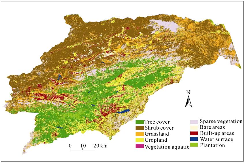
Fig. 4 Land-cover map of Nzhelele and Levhuvu catchments, South Africa in 2017–2018
plantation, and open water surface accounts for 18.86% 61.38%, and 66.67%, respectively.
of catchments, which indicated that land-cover in these According to the confusion matrix in Table 2, the
catchments were changed somehow by human activities. proportions of misclassification can be derived for each
The southern part of the river catchments has more land-cover type. For instance, 20.18% grassland sam-
dense and green vegetation (tree cover and plantations), ples (180 samples out of 892 total samples) were classi-
as opposed to the northern parts with mostly shrubs, fied as shrub cover and 13.19% (123 samples out of 892
sparse vegetation and grasslands. Similarly cropland is total samples) were classified as cropland. In this study,
more noticeable in the southern parts as opposed to the cropland was mixed with tree cover, shrub cover, and
northern parts. The built-up areas pattern is also more grassland, 10.16% (91 samples out of 896 total sam-
concentrated in the southern part of the catchments as ples), 6.58% (59 samples out of 896 total samples) and
opposed to the north. 7.81% (70 samples out of 896 total samples) of cropland
samples were wrong classified as tree cover, shrub
3.2 Accuracy assessment result cover, and grassland. A certain percentage of samples
A total of 8154 validation samples generated by GEE, for all land-cover classes except plantation were mis-
including 890 samples of tree cover, 861 samples of classified as grassland, ranging from 1.50% for water
shrub cover, 892 samples of grassland, 896 samples of surface to 13.01% for shrub cover. Total of 20.18%,
cropland, 191 samples of vegetation aquatic, 901 sam- 9.77% and 6.58% of grassland, sparse vegetation, and
ples of sparse vegetation, 877 samples of bare areas, 871 cropland samples were incorrectly classified as shrub
samples of built-up areas, 868 samples of water surface, cover. The 13.79% of grassland samples were misclassi-
and 907 samples of plantation. fied as cropland.
The overall accuracy of land-cover map was 76.43%
(Table 2). Among the classes, plantation has the highest 4 Discussion
accuracies of classification (97.68% for the PA and
95.47% for the UA), following by water surface, tree 4.1 Classification results comparison with existing
cover, built-up areas, bare areas, and sparse vegetation products
with user accuracy of 89.63%, 82.32%, 77.95%, 77.87% The Overall Accuracy (OA) of land-cover in the study is
and 77.70%. The land types of grassland, cropland, 76.43% that is acceptable compared with the existing global
shrub cover, and vegetation aquatic were poorly classi- products, e.g., FROM-GLC30, FROM-GL10, GlobeLand30
fied. Among them, the PA of grassland, vegetation and African continental level land-cover produced by
aquatic, cropland and shrub cover were 44.39%, 57.07%, Stacked Autoencoder (SAE) approach (Li et al., 2016).ZENG Hongwei et al. A Synthesizing Land-cover Classification Method Based on Google Earth Engine: A Case… 405
Table 2 Confusion table for the land-cover map of Nzhelele and Levhuvu catchments in South Africa with random forest
Land-cover TC SC GR CR VA SV BA BU WS PL Sum PA (%)
TC 810 0 19 26 0 1 0 2 0 32 890 91.01
SC 1 574 112 51 0 81 7 35 0 0 861 66.67
GR 46 180 396 123 1 43 44 51 4 4 892 44.39
CR 91 59 70 550 1 56 34 29 0 6 896 61.38
VA 1 0 10 3 109 0 16 9 43 0 191 57.07
SV 6 88 41 46 0 683 16 21 0 0 901 75.80
BA 0 2 14 5 10 0 760 50 36 0 877 86.66
BU 0 29 16 35 2 15 52 721 1 0 871 82.78
WS 12 9 13 18 19 0 47 7 743 0 868 85.60
PL 17 0 0 0 2 0 0 0 2 886 907 97.68
Sum 984 941 691 857 144 879 976 925 829 928 8154
UA (%) 82.32 61.00 57.31 64.18 75.69 77.70 77.87 77.95 89.63 95.47 76.43
Notes: TC = Tree cover, SC = Shrub cover, GR = Grassland, CR = Cropland, VA = Vegetation aquatic, SV = Sparse vegetation, BA = Bare areas, BU = Built-up
areas, WS = Water surface, PL = Plantation. PA is producer accuracy; UA is user accuracy
The OA of FROM-GLC30 largely changes with the Shrub cover and grassland were poorly classified
classifier used in the product. In specific, the accuracy compared to other categories of Nzhelele and Levhuvu
of FROM-GLC30 is 64.89% for the support vector ma- catchments, and the PA and UA of shrubs and grassland
chines, 59.83% for the random forest classifier, 57.88% are 66.67% and 61.00%, 44.39% and 57.13% (Table 3).
for J48 decision tree classifier, and 53.88% for maxi- However, compared to FROM-GLC30, SAE African
mum likelihood classification (Gong et al., 2013). The land-cover, FROM-GLC10, and GlobeLand30, the ac-
OA of FROM-GL10 is 72.76% for random forest classi- curacy of them is also comparable and acceptable.
fier (Gong et al., 2019), and the OA of GlobeLand30 in Taken shrub cover as example, the PA of shrub cover in
2010 is 80.33% based on the integration of pixel- and Nzhelele and Levhuvu catchments was better than
object-based methods with knowledge (Chen et al., FROM-GLC30, FROM-GLC10, only slightly lower
2015). At the African continental, land-cover produced than FROM-GLC10 (Table 3), the UA of it was better
by Li et al. (2016) indicated that the OA of the than FROM-GLC30, SAE African land-cover, while
land-cover with 30 m Landsat imagery in 2014 is lower than FROM-GLC10 and GlobeLand30. Taken
76.03% for random forest classifier, 77.74% for support grassland as example, the PA of grassland was better
vector machines, 77.86% for artificial neural networks, than FROM-GLC30, SAE African land-cover, and
and 78.99% with stacked auto-encoder. The OA of our lower than FROM-GLC10, the UA of it was better than
result is 76.43% (Table 2) that is higher than FROM- FROM-GLC30, while lower than SAE African
GLC30 (maximum OA of 64.89%), FROM-GLC10 (OA land-cover, FROM-GLC10, and GlobeLand30.
of 72.76%), close to African continental level land-
cover (OA of 76.03%) of Li et al. (2016), while is lower 4.2 Role of Sentinel-1 in land-cover classification
than GlobeLand30 (OA of 80.33%). The accuracy of To evaluate the contribution of Sentinel-1 on land
land-cover product is greatly varied at country level, and type classification, we tested the classification with-
South Africa is the one of worst classified country in the out using Sentinel-1. The result of test is shown in
land-cover of FROM-GLC30 with the OA below 50% Table 4. The overall accuracy of land-cover classifi-
(Gong et al., 2013). Nzhelele and Levhuvu catchments cation was 76.07%, which was slightly lower than the
is one part of South Africa, the OA of land-cover based result including Sentinel-1 (76.43%, Table 2). This
on our synthesizing approach reached to 76.43%, and it indicates that integration of sentinel-1 data into the
is evident that the synthesizing approach in this study is classifier slightly improve accuracy of land-cover
acceptable and can be used for land-cover mapping. classification.406 Chinese Geographical Science 2020 Vol. 30 No. 3
Table 3 Accuracy comparison our result with Finer Resolution (30 m) Observation and Monitoring of Global Land-cover
(FROM-GLC30), Stacked Autoencoder (SAE) African land-cover, Finer Resolution (10 m) Observation and Monitoring of Global
Land-cover (FROM-GLC10), and GlobaLand30
Shrub cover Grassland
Land-cover product Overall accuracy (%)
Producer accuracy (%) User accuracy (%) Producer accuracy (%) User accuracy (%)
FROM-GLC30 (Gong et al., 2013) 64.89 49.65 33.94 44.13 34.88
SAE African land-cover (Li et al., 2016) 76.03 66.82 57.85 38.48 45.42
FROM-GLC10 (Gong et al., 2019) 72.76 62.75 64.49 58.51 50.77
GlobeLand30 (Chen et al., 2015) 80.33 – 72.64 – 72.16
Result of this study 76.43 66.67 61.00 57.13 44.39
Table 4 Accuracy assessment for the land-cover map of Nzhelele and Levhuvu catchments without Sentinel-1
RF TC SC GR CR VA SV BA BU WS PL Sum PA (%)
TC 812 0 14 27 0 2 0 2 0 33 890 91.24
SC 1 587 103 38 1 87 10 34 0 0 861 68.18
GR 48 198 388 115 3 43 38 51 5 3 892 43.50
CR 94 81 64 500 1 69 30 51 0 6 896 55.80
VA 2 1 10 3 108 0 15 10 42 0 191 56.54
SV 6 89 35 45 0 691 16 19 0 0 901 76.69
BA 0 5 9 10 10 0 769 39 35 0 877 87.69
BU 1 23 17 39 1 14 49 726 1 0 871 83.35
WS 12 14 17 10 21 1 47 10 735 1 868 84.68
PL 16 0 0 0 3 0 0 0 1 887 907 97.79
Sum 992 998 657 787 148 907 974 942 819 930 8154
UA (%) 81.85 58.82 59.06 63.53 72.97 76.19 78.95 77.07 89.74 95.38 76.07
Note: the meaning of the abbreviation is as same as in Table 2
The influence of Sentinel-1 on land-cover classifica- UA and PA for different categories, the integration of
tion is varied to specific land-cover type. According to Sentinel-1 data into the classifier should be carefully
the Table 2 and Table 4, the user and producer accuracy assessed for specific land-cover types.
difference for each land-cover type with or without Sen-
tinel-1 was shown in Fig. 5. In our study, the accuracy
of cropland and vegetation aquatic with Sentinel-1 im-
proved significantly, their PA and UA was improved by
5.58% and 0.52%, 0.64% and 2.67%, respectively com-
pared to that without Sentinel-1. While the accuracy of
bare areas with Sentinel-1 was slightly lower than the
result without using Sentinel-1, the UA and PA of it with
Sentinel-1 decreased by 1.03% and 1.08%. Using Sen-
tinel-1 data also improved the UA of tree cover, shrub
cover, sparse vegetation, built-up areas and plantation
by 0.46%, 2.18%, 1.52%, 0.88%, and 0.10%, while re- Fig. 5 Accuracy difference between land-cover with and with-
duced their PA by 0.22%, 1.51%, 0.89%, 0.57%, and out Sentinel-1. (The meaning of the abbreviation is shown in
0.11%, respectively. Considering the accuracy change of Table 2)ZENG Hongwei et al. A Synthesizing Land-cover Classification Method Based on Google Earth Engine: A Case… 407
4.3 Role of spectral indices is unclear. To highlight the advantage of stratified sam-
In order to enhancing the distinguishing of different pling method used in the model, accuracy of land type
land-cover types, NDVI, EVI, SAVI, NDBI, and NDWI classification was evaluated by using the same number
were integrated into random forest classifier, how is the of samples in training and validation generated by the
impact of them on land-cover classification? This study random sampling method (Table 5).
tested the land-cover accuracy without NDVI, EVI, Table 5 shows that the OA of land-cover from ran-
SAVI, NDBI, and NDWI, respectively. The result shows dom sampling reached to 81.77%, which is generally
that overall accuracy of classification without NDVI, higher than the result using the stratified sampling
EVI, and SAVI were 76.39%, 76.55%, and 76.54%, re- method (Table 2). The UA and PA of tree cover, shrub,
spectively that was close to the results (Table 2) using water surface, and plantation from the random sampling
the all spectral indices. Similar result was observed in were above 80%. In particular, the UA and PA of shrub
the classification of built-up areas, the accuracy of cover from random sampling were significantly higher
built-up areas has little change. The possible reason for 28.78% and 24.71% than that from stratified sampling
little change of accuracy was that the above indices method. The UA and PA of tree cover from random
were calculated using bands of Landsat 8 OLI while sampling were also higher 1.1% and 6.98% than that
these bands participated in the training process (Fig. 2). from stratified sampling method.
The participation of NDWI has positive effect on the However, the under-fitting problems were observed
accuracy of water surface identification that the PA and in the non-dominant land-cover types from random
UA of water surface increased from 85.14% and 89.25% sampling method. In this study, UA of grassland, crop-
to 85.60% and 89.63% using NDWI. lands, vegetation aquatic, sparse vegetation, bare areas,
and built-up areas from the random sampling in Table 5
4.4 Accuracy difference of different sampling were much lower than that from stratified sampling
method method in Table 2. In particular, the PA of cropland,
The accuracy of land-cover classification is sensitive to vegetation aquatic, sparse vegetation, bare areas, and
the number and distribution of land-cover samples built-up areas from random sampling sharply decreased
(Gong et al., 2019). In this work, the stratified sampling to 0 (Table 5). The extreme imbalance of samples for
method was employed to generate the roughly equal different land types was the possible reason for worse
samples for each category. Whether this stratified sam- classified of non-dominant land types. Compared with
pling method is beneficial for land-cover classification stratified sampling method, random sampling generates
Table 5 Accuracy assessment for the land-cover map of Nzhelele and Levhuvu catchments in South Africa with random sampling
RF TC SC GR CR VA SV BA BU WS PL Sum PA (%)
TC 642 15 39 2 0 0 0 0 0 10 708 90.68
SC 10 3601 126 4 0 0 0 0 0 0 3741 96.26
GR 47 498 307 11 0 0 0 0 2 2 867 35.41
CR 33 95 52 30 0 0 0 0 0 2 212 14.15
VA 0 0 1 0 0 0 0 0 0 0 1 0.00
SV 0 59 2 0 0 1 0 0 0 0 62 1.61
BA 0 1 2 0 0 0 0 0 0 0 3 0.00
BU 0 9 6 0 0 0 0 0 0 0 15 0.00
WS 0 1 2 0 0 0 0 0 25 0 28 89.29
PL 9 0 1 0 0 0 0 0 0 62 72 86.11
Sum 741 4279 538 47 0 0 0 0 27 76 5709
UA (%) 86.64 84.16 57.06 63.83 – 100.00 – 0.00 92.59 81.58 81.77
Note: the meaning of the abbreviation is as the same as in Table 2408 Chinese Geographical Science 2020 Vol. 30 No. 3
samples according to the proportion of land types in vegetation indices has little effect on final land-cover
existing product. This leads to most of samples concen- classification result.
trate in the dominant land-cover types while the samples
are insufficient of non-dominant land-cover types, and References
causes the under-fitting of them.
Arino O, Gross D, Ranera F et al., 2007. GlobCover: ESA service
5 Conclusions for global land cover from MERIS. In 2007 IEEE Interna-
tional Geoscience and Remote Sensing Symposium,
2412–2415.
This paper designed a feasible land-cover classification
Breiman L, 2001. Random Forests. Machine Learning, 45(1):
method for the areas with insufficient ground samples. 5–32. doi:10.1023/A:1010933404324
Based on the Google Earth Engine platform, this Chen B, Xiao X, Li X et al., 2017. A mangrove forest map of
method take Landsat 8 OLI, Sentinel-1 GRD and terrain China in 2015: analysis of time series Landsat 7/8 and Senti-
data as data source, use random forest classifier to clas- nel-1A imagery in Google Earth Engine cloud computing
platform. ISPRS Journal of Photogrammetry and Remote
sify land-cover. Two new strategies were used in this
Sensing, 131: 104–120. doi:https://doi.org/10.1016/j.isprsjprs.
approach, one is using percentile and monthly median 2017.07.011
composites to expand input metrics of classifier, and Chen J, Chen J, Liao A et al., 2015. Global land cover mapping at
another is using stratified sampling method to generate 30m resolution: a POK-based operational approach. ISPRS
the training and validation samples from the existing Journal of Photogrammetry and Remote Sensing, 103: 7–27.
doi: https://doi.org/10.1016/j.isprsjprs.2014.09.002
land-cover product that overcome the defect of insuffi-
Dong J, Xiao X, Menarguez M A et al., 2016. Mapping paddy rice
cient ground data.
planting area in northeastern Asia with Landsat 8 images,
Based on this method, the 30-m land-cover with 10 phenology-based algorithm and Google Earth Engine. Remote
classes of Nzhelele and Levhuvu catchments, South Af- Sensing of Environment, 185: 142–154. doi: https://doi.org/
rica in 2017–2018 was classified, and the overall accu- 10.1016/j.rse.2016.02.016
racy of the land-cover reached to 76.43%. The planta- Friedl M A, McIver D K, Hodges J C F et al., 2002. Global land
cover mapping from MODIS: algorithms and early results.
tion, water surface, tree cover, bare areas, built-up areas,
Remote Sensing of Environment, 83(1): 287–302. doi:
and sparse vegetation were classified well with their https://doi.org/10.1016/S0034-4257(02)00078-0
user accuracy and producer accuracy was above 75%. Funk C, Peterson P, Landsfeld M et al., 2015. The climate hazards
The result in this study is comparable and acceptable to infrared precipitation with stations—a new environmental re-
the existing land-cover products and can be used for cord for monitoring extremes. Scientific Data, 2(1): 150066.
land-cover mapping in the area with insufficient ground doi:10.1038/sdata.2015.66
Gong P, Liu H, Zhang M et al., 2019. Stable classification with
samples.
limited sample: transferring a 30-m resolution sample set col-
Further evaluation confirmed that Sentinel-1 has the lected in 2015 to mapping 10-m resolution global land cover
positive impact on the overall accuracy of land-cover in 2017. Science Bulletin, 64(2095–9273): 370–373.
classification, and can slightly improve the overall ac- doi:https://doi.org/10.1016/j.scib.2019.03.002
curacy of land-cover. However, its contribution on Gong P, Wang J, Yu L et al., 2013. Finer resolution observation
land-cover classification varied with land types that and monitoring of global land cover: first mapping results with
Landsat TM and ETM+ data. International Journal of Remote
mean it should be carefully assessed the performance for
Sensing, 34(7): 2607–2654. doi:10.1080/01431161.2012.
specific land type when using Sentinel-1 data into clas-
748992
sification process. In addition, the results highlights the Gorelick N, Hancher M, Dixon M et al., 2017. Google Earth En-
importance of sampling method on the influence on gine: planetary-scale geospatial analysis for everyone. Remote
land-cover classification, the unfitting problem would Sensing of Environment, 202: 18–27. doi:https://doi.org/
be happened in the classification of non-dominant cate- 10.1016/j.rse.2017.06.031
Hansen M C, Potapov P V, Moore R et al., 2013. High-Resolution
gories when using random sampling method. In order to
Global Maps of 21st-Century Forest Cover Change. Science,
ensure the classification accuracy of non-dominant land
342(6160): 850. doi:10.1126/science.1244693
types, stratified sampling method is recommended in the Huete A, Didan K, Miura T et al., 2002. Overview of the radio-
land-cover classification. When related reflectance metric and biophysical performance of the MODIS vegetation
bands participated in the training process, individual indices. Remote Sensing of Environment, 83(1): 195–213.ZENG Hongwei et al. A Synthesizing Land-cover Classification Method Based on Google Earth Engine: A Case… 409 doi:https://doi.org/10.1016/S0034-4257(02)00096-2 Singha M, Dong J, Zhang G et al., 2019. High resolution paddy Huete A R, 1988. A soil-adjusted vegetation index (SAVI). Re- rice maps in cloud-prone Bangladesh and Northeast India us- mote Sensing of Environment, 25(3): 295–309. doi:https://doi. ing Sentinel-1 data. Scientific data, 6(1): 1–10. doi:10.1038/ org/10.1016/0034-4257(88)90106-X s41597-019-0036-3 Huete A R, Liu H Q, Batchily K et al., 1997. A comparison of Tian F, Wu B, Zeng H et al., 2019. Efficientidentification of corn vegetation indices over a global set of TM images for cultivation area with multitemporal Synthetic Aperture Radar EOS-MODIS. Remote Sensing of Environment, 59(3): and optical images in the Google Earth Engine Cloud Plat- 440-451. doi:https://doi.org/10.1016/S0034-4257(96)00112-5 form. Remote Sensing, 11(6). doi:10.3390/rs11060629 Li W, Fu H, Yu L et al., 2016. Stacked Autoencoder-based deep Tucker C J, 1979. Red and photographic infrared linear combina- learning for remote-sensing image classification: a case study tions for monitoring vegetation. Remote Sensing of Environ- of African land-cover mapping. International Journal of Re- ment, 8(2): 127–150. doi:https://doi.org/10.1016/0034-4257 mote Sensing, 37(23): 5632–5646. doi:10.1080/01431161. (79)90013-0 2016.1246775 Wang J, Zhao Y, Li C et al., 2015. Mapping global land cover in Liu H Q, Huete A, 1995. A feedback based modification of the 2001 and 2010 with spatial-temporal consistency at 250m NDVI to minimize canopy background and atmospheric noise. resolution. ISPRS Journal of Photogrammetry and Remote IEEE Transactions on Geoscience and Remote Sensing, 33(2): Sensing, 103: 38–47. doi:https://doi.org/10.1016/j.isprsjprs. 457–465. doi:10.1109/TGRS.1995.8746027 2014.03.007 Makungo R, Odiyo J O, Ndiritu J G et al., 2010. Rainfall-runoff Xiong J, Thenkabail P S, Gumma M K et al., 2017. Automated modelling approach for ungauged catchments: a case study of cropland mapping of continental Africa using Google Earth Nzhelele River sub-quaternary catchment. Physics and Chem- Engine cloud computing. ISPRS Journal of Photogrammetry istry of the Earth, Parts A/B/C, 35(13): 596–607. doi:https:// and Remote Sensing, 126: 225–244. doi:https://doi.org/ doi.org/10.1016/j.pce.2010.08.001 10.1016/j.isprsjprs.2017.01.019 McFeeters S K, 1996. The use of the Normalized Difference Wa- Xu H, 2006. Modification of normalised difference water index ter Index (NDWI) in the delineation of open water features. (NDWI) to enhance open water features in remotely sensed International Journal of Remote Sensing, 17(7): 1425–1432. imagery. International Journal of Remote Sensing, 27(14): doi:10.1080/01431169608948714 3025–3033. doi:10.1080/01431160600589179 Miller J D, Thode A E, 2007. Quantifying burn severity in a het- Xu H, 2008. A new index for delineating built-up land features in erogeneous landscape with a relative version of the delta satellite imagery. International Journal of Remote Sensing, Normalized Burn Ratio (dNBR). Remote Sensing of Environ- 29(14): 4269–4276. doi:10.1080/01431160802039957 ment, 109(1): 66–80. doi:https://doi.org/10.1016/j.rse.2006. Yu L, Wang J, Li X et al., 2014. A multi-resolution global land 12.006 cover dataset through multisource data aggregation. Science Pekel J F, Cottam A, Gorelick N et al., 2016. High-resolution China Earth Sciences, 57(10): 2317–2329. doi:10.1007/ mapping of global surface water and its long-term changes. s11430-014-4919-z Nature, 540: 418. doi:10.1038/nature20584 Zha Y, Gao J, Ni S, 2003. Use of normalized difference built-up Pesaresi M, Ehrlich D, Ferri S et al., 2016. Operating procedure index in automatically mapping urban areas from TM imagery. for the production of the Global Human Settlement Layer from International Journal of Remote Sensing, 24(3): 583–594. Landsat data of the epochs 1975, 1990, 2000, and 2014. Pub- doi:10.1080/01431160304987 lications Office of the European Union, 1–62. Zhang X, Wu B, Ponce-Campos E G et al., 2018. Mapping Savitzky A, Golay M J E, 1964. Smoothing and differentiation of up-to-date paddy rice extent at 10 m resolution in China through data by simplified least squares procedures. Analytical Chem- the Integration of optical and Synthetic Aperture Radar Images. istry, 36(8): 1627–1639. doi:10.1021/ac60214a047 Remote Sensing, 10(8): 1200. doi:10.3390/rs10081200
You can also read