Brief communication: Updated GAMDAM glacier inventory over high-mountain Asia - The Cryosphere
←
→
Page content transcription
If your browser does not render page correctly, please read the page content below
The Cryosphere, 13, 2043–2049, 2019
https://doi.org/10.5194/tc-13-2043-2019
© Author(s) 2019. This work is distributed under
the Creative Commons Attribution 4.0 License.

Brief communication: Updated GAMDAM glacier inventory
over high-mountain Asia
Akiko Sakai
Graduate School of Environmental Studies, Nagoya University, Nagoya, Japan

Correspondence: Akiko Sakai (shakai@nagoya-u.jp)

Received: 4 July 2018 – Discussion started: 20 July 2018
Revised: 9 June 2019 – Accepted: 24 June 2019 – Published: 19 July 2019

Abstract. The original Glacier Area Mapping for Discharge         on a large-scale glacier inventory, highlighting the need for
from the Asian Mountains (GAMDAM) glacier inventory               accurate, high-quality coverage of the entire HMA region.
was the first methodologically consistent dataset for high-       Specifically, precise glacier inventories are needed for mod-
mountain Asia. Nonetheless, the GAMDAM inventory un-              elling total glacier volume (Frey et al., 2014; Farinotti et al.,
derestimated glacier area, as it did not include steep ice- and   2019), deriving volume change from altimetry and digital
snow-covered slopes or shaded components. During revision         elevation maps (DEMs, e.g. Brun et al., 2017) and surface-
of the inventory, Landsat imagery free of shadow, cloud,          flow velocity (Dehecq et al., 2019), establishing changes in
and seasonal snow cover was selected for the period 1990–         snow cover and albedo (Naegeli et al., 2019), catchment-
2010, after which > 90 % of the glacier area was delineated.      and regional-scale hydrologic modelling (e.g. Immerzeel et
The updated GAMDAM inventory, comprised of 453 Land-              al., 2010), projecting future glacier configuration (Huss and
sat images, includes 134 770 glaciers with a total area of        Hock, 2015; Shannon et al., 2019), and assessing uncer-
100 693 ± 11 790 km2 .                                            tainty in estimates of glacier-surface elevation change (e.g.
                                                                  Nuimura et al., 2012; Bolch et al., 2017).
                                                                     While the Randolph Glacier Inventory (RGI) (Arendt et
                                                                  al., 2015; RGI Consortium, 2017) was the first database with
1   Introduction                                                  global coverage, the record exhibits considerable variability
                                                                  in accuracy even within HMA. Regional databases include
Glaciers in high-mountain Asia (HMA) play a significant           the second Chinese glacier inventory (hereafter the CGI2),
role as a water resource for people living downstream (Im-        produced by automatic delineation with manual correction
merzeel et al., 2010; Bolch et al., 2012). Glacier recession      (Guo et al., 2015), and the NM18 inventory for the Karako-
in recent decades has contributed to sea level rise, and this     ram and Pamir region (Mölg et al., 2018), derived from auto-
trend is anticipated to continue in the future (Huss and Hock,    mated digital mapping and corrected manually by the coher-
2015; Marzeion et al., 2018; Radić and Hock, 2013). Re-          ence of synthetic aperture radar (SAR) imagery for debris-
cent analysis of surface elevation change has revealed that       covered glaciers (Frey et al., 2012). The latter study also
glaciers in HMA exhibit contrasting behaviour (Brun et al.,       made separate delineations for all debris-covered areas.
2017; Gardner et al., 2013; Kääb et al., 2012, 2015): those          Between February 2011 and March 2014, the Glacier Area
in the Himalaya and the eastern Nyainqêntanglha Mountains         Mapping for Discharge from the Asian Mountains (GAM-
are shrinking rapidly, while the Karakoram and West Kunlun        DAM) project compiled a glacier inventory for HMA, cover-
glaciers are in balance or show a slight mass gain. Accord-       ing the region between 27.0 and 54.9◦ N in latitude and 67.4
ingly, a recent climate analysis for those areas demonstrated     and 103.9◦ E in longitude. In its first iteration, published in
that the Karakoram and West Kunlun regions are relatively         2015, the GAMDAM glacier inventory (GGI) did not include
stable under global warming conditions, being less sensitive      steep ice- and snow-covered slopes. Moreover, where winter-
to temperature change (Sakai and Fujita, 2017). This assess-      time imagery was employed to avoid summer monsoon cloud
ment of both glacier volume and climatic conditions is based

Published by Copernicus Publications on behalf of the European Geosciences Union.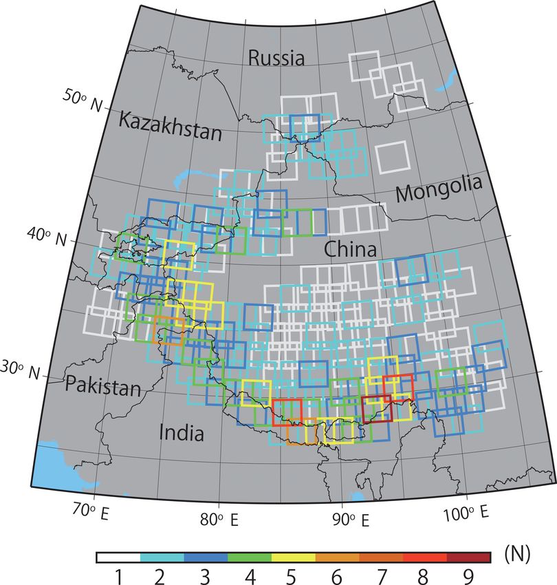
2044                                             A. Sakai: Updated GAMDAM glacier inventory over high-mountain Asia

cover, shaded areas of glacier surfaces were excluded from
the inventory (Fig. S1a in the Supplement). To help address
these shortcomings, I present a revised glacier inventory
for HMA based on summertime (May–September) imagery,
exhibiting clear glacier boundaries for steep, snow-covered
slopes and shaded areas. The abbreviated terms GGI15 and
GGI18 refer to the first version of the GGI (Nuimura et al.,
2015) and the current, updated version (this study), respec-
tively.

2     Data

I utilized a total of 453 Landsat 5 Thematic Mapper™
and Landsat 7 Enhanced Thematic Mapper Plus (ETM+)
level 1T scenes derived from 196 USGS EarthExplorer
path–row sets (http://earthexplorer.usgs.gov/, last access:
17 July 2019). Landsat ID and acquisition dates were used
to delineate glacier outlines and are summarized in Table S1
in the Supplement. Due to the challenge of obtaining sum-
mertime imagery for the 1999–2003 setting period (Nuimura
et al., 2015) that is free of clouds, seasonal snow cover, and
shadows, the annual search range was expanded to 1990–
                                                                  Figure 1. Footprints of the Landsat scenes used in the GGI18.
2010 and the monthly search range to May–September (i.e.          Colours indicate the number of scenes used to delineate glacier out-
the high-solar-angle season). Where part of a glacier sur-        lines.
face was obscured by cloud or snow, the Landsat archive
was searched for more viable images covering that partic-
ular site; for glaciers with steep headwalls, images were se-     GGI18, I selected an additional two images (Fig. S1b and
lected with the most clearly defined glacier outlines (full de-   c) with minimal snow and no cloud cover over the target
tails of this methodological approach are given in Sect. 3).      glaciers (Fig. S1). Focusing on the steep snow-covered head-
As a result, the GGI18, like its predecessor, contains single     walls of the Khumbu Glacier (purple ellipses in right panels,
path–row scenes comprised of multiple images (Fig. 1). Fi-        Fig. S1), the image displayed in Fig. S1b exhibits the least
nally, the GGI18 employs the ASTER-GDEM2 to analyse               seasonal snow cover and provides the sharpest boundaries
the glacier aspect in each 90 m×90 m grid.                        among the four additional images, and thus this was utilized
                                                                  in the GGI18.
                                                                     Ultimately, the degrees of cloud and snow cover and the
3     Methods
                                                                  clarity of glacier outlines are the key factors in selecting
Unlike seasonal snow cover, glaciers are considered to be         suitable Landsat imagery for glacier delineation. The most
permanent snow and ice. It is vital, therefore, that seasonal     challenging sites are those for which the glacier headwall
snow coverage is excluded from each glacier polygon. In ad-       comprises at least part of the accumulation area; to delineate
dition, to help quantify the glacial contribution to sea level    such glaciers accurately, I focused on unambiguous bound-
change and water resources, polygons must include all areas       aries on north-facing walls. Nonetheless, in regions domi-
in which fluctuations in surface elevation reflect changes in     nated by summer monsoonal precipitation, such as the east-
ice mass.                                                         ern Himalaya and eastern Nyainqêntanglha Mountains, the
                                                                  approach described here was inadequate to locate appropri-
3.1    Selection of Landsat imagery                               ate imagery (see Sect. 4.3).

As detailed in Sect. 2, I expanded the search period to ob-       3.2   Manual delineation
tain Landsat images in which glacier outlines are depicted
clearly. Figure S1, for example, shows the five images se-        Owing to the many debris-covered glaciers in HMA (e.g.
lected to delineate glacier outlines in the accumulation zone     Herreid et al., 2015; Minora et al., 2016; Nagai et al., 2016;
of the Khumbu Glacier, in the Nepalese Himalaya. While            Ojha et al., 2017), for which automatic detection using the
the cloud-free image in Fig. S1a was utilized for the GGI15,      band ratio method is not possible (Paul et al., 2002), all
large areas of the glacier surface lie in shadow, thus preclud-   glacier outlines included in the GGI18 were delineated man-
ing accurate delineation. Therefore, during revision for the      ually. Using the newly selected Landsat imagery, I modified

The Cryosphere, 13, 2043–2049, 2019                                                    www.the-cryosphere.net/13/2043/2019/
A. Sakai: Updated GAMDAM glacier inventory over high-mountain Asia 2045
the GGI15 glacier polygons following the method described 3.3 Uncertainties in glacier area
by Nuimura et al. (2015) but with two important differences.
First, whereas glaciers of < 0.05 km2 in area were excluded Revision of glacier outlines and subsequent delineation test-
from the GGI15 (Nuimura et al., 2015), the minimum glacier ing were both performed by the author. Delineation tests
area in the GGI18 is 0.01 km2 so as to account for the numer- were conducted on 10 debris-covered glaciers and 12 debris-
ous small glaciers separated by dividing ridges. Furthermore, free glaciers using a total of 10 Landsat images (listed in Ta-
I included small glaciers as much as possible during the re- ble S4), which included shaded (winter), snow-covered, and
vision process. A total of 10 grid cells (= 0.009 km2 ) were partially cloud-covered scenes. Since fully cloud-obscured
used as a guide for measuring area. In contrast to the GGI15, images were not used in the delineation process, I did not se-
in which glacier outlines were delineated manually by 11 in- lect such glacier outlines in the testing process. Furthermore,
dividuals (Nuimura et al., 2015), all of the delineation for the I did not utilize Google Earth imagery since the resolution is
GGI18 was conducted by a single person. not regionally uniform throughout HMA (see Sect. 3.2). For
The second methodological difference between the GGI15 each Landsat image, I created a single glacier outline and
and the GGI18 relates to steep headwalls. Nuimura et calculated the normalized standard deviation (NSD: standard
al. (2015) excluded steep snow- and ice-covered slopes from deviation divided by average glacier area) for each glacier
the GGI15, arguing that glaciers on high-angle headwalls area (e.g. Fig. S4). For each area class, the NSD increases
generally do not undergo changes in surface elevation re- with decreasing glacier area (Fig. S5). Moreover, NSD val-
lated to mass fluctuations. Those authors also underestimated ues are higher for debris-covered glaciers than for debris-
the scale of upper glacier headwalls that are mantled with free glaciers (particularly for smaller glaciers), although
snow or ice. In contrast, since I was able to obtain com- the GGI18 does not classify debris-covered and debris-free
paratively distinct outlines for those glaciers with relatively glaciers.
thick ice on steep headwalls, the GGI18 includes the snow- The proportion of debris-covered glaciers in each area
or ice-covered parts of the glacier surface. For instance, class in the eastern Himalaya (27.5–29.0◦ N, 85.0–92.0◦ E)
Fig. S2a depicts the high-angle, avalanche-prone headwall (Ojha et al., 2017) (Fig. S6) was applied for all of the study
of the Trakarding Glacier in 2016, on which hanging glaciers areas (HMA), then they were used to calculate the number-
are clearly visible. Thanks to their distinct outlines, these fea- weighted average NSD of glacier area for each glacier area
tures are also identifiable on the 1999 Landsat image (arrows, class, including both debris and debris-free glaciers (Fig. S6).
Fig. S2b), indicating that they are long-term components of Here, the NSDs of the glacier area were assumed to be 15 %
the glacier system and thus need to be included in the inven- for smaller (< 0.25 km2 ) debris-free glaciers and 30 % for
tory. smaller (< 2 km2 ) debris-covered glaciers based on Fig. S5.
The correct distinction between debris-covered glaciers NSD for all glaciers in Fig. S6 was assumed to be the un-
and rock glaciers is a challenge, as gradual transitions can certainty in glacier area for all types of glacier (including
exist under permafrost conditions (Mölg et al., 2018). Rock debris-covered and debris-free). Finally, the maximum NSD
glaciers have terrain with ridges and furrow surface pat- 19 % was found for glaciers of 1–2 km2 in area (Fig. S6).
terns (Bodin et al., 2010), while debris-covered glaciers
have ponds surrounded by ice cliffs. Those detailed topogra-
4 Results and discussion
phies were difficult to detect via Landsat imagery because
of its relatively low resolution. Therefore, debris-covered ar- The GGI15 reported a total glacier area of 91 263 ±
eas were determined from high-resolution Google Earth im- 13 689 km2 (Nuimura et al., 2015), which included the com-
agery. Specifically, those portions of the glacier surface ex- bined area of holes in glacier polygons. Excluding polygon
hibiting rock-glacier-like topography (e.g. flow lobes) were holes, I recalculated the total glacier area in the GGI15 as
identified visually and omitted (see Fig. S3). As for the 87 583 ± 3137 km2 (Table 1), while the GGI18 is comprised
debris-covered glaciers in the eastern Himalaya and eastern of 134 770 glaciers with a total area of 100 693 ± 11 790 km2
Nyainqêntanglha Mountains, crevassed surfaces can be de- (Table 1). Hence, the total glacier area and glacier number
tected even in the snow-covered glacier surface using high- for HMA are 13 % and 35 % greater in the GGI18 than in the
resolution Google Earth imagery. For regions where high- GGI15, respectively.
resolution Google Earth imagery is unavailable (e.g. east-
ern Himalaya and eastern Nyainqêntanglha Mountains) or 4.1 Comparison with the GGI15
the glacier surface is obscured by seasonal snow cover (e.g.
Karakoram and Pamir), I employed a combination of con- Following the region delimitation of RGI 6.0 (Arendt et al.,
tours and surface–colour difference between glacier areas 2015; RGI Consortium, 2017), the aggregated polygon files
and glacier-free areas to delineate debris-covered glaciers. for the GGI18 are divided into four regions: Central Asia,
South Asia (east), South Asia (west), and North Asia (lim-
ited by the Sayan and Altai mountains). Regional differences
in glacier area among the GGI18, GGI15, and RGI 6.0 are
www.the-cryosphere.net/13/2043/2019/ The Cryosphere, 13, 2043–2049, 20192046 A. Sakai: Updated GAMDAM glacier inventory over high-mountain Asia
Table 1. Comparison of the GGI15 and GGI18 inventories in terms of the total glacier area, glacier area ratio based on summer imagery, and
based on imagery acquired between 1999 and 2001.
Minimum glacier Total glacier Total number Number of Glacier area Glacier area based
area (km2 ) area (km2 ) of glaciers Landsat images based on summer on images acquired
employed (JJAS) images (%) from 1999 to 2001 (%)
GGI15 (Nuimura et al., 2015) 0.05 87 583 ± 13 137 87 084 356 69 73
GGI18 (this study) 0.01 100 693 ± 11 790 134 770 453 95 48
summarized in Table S2 (note that the RGI 6.0 incorpo- 4.2 Comparison with the CGI2 and NM18 inventories
rated part of the GGI15; RGI Consortium, 2017). For all re-
gions, glacier area in the GGI18 is > 10 % greater than in the To assess the GGI18 relative to the CGI2 (Guo et al., 2015)
GGI15, with the greatest differences in eastern South Asia and NM18 (Mölg et al., 2018) inventories, I extracted the two
(+18 %) and western South Asia (+16 %). Both eastern and components of the GGI18 covered by the respective domains
western South Asia cover portions of the high Himalaya, in- of the other datasets. A direct comparison of the three re-
cluding abundant high-relief glaciated headwalls, indicating veals that the GGI18-derived glacier area is smaller than that
that the GGI15 underestimated glacier area most in shaded of the CG12 for elevations of 4000–5500 m (Fig. S11a) and
areas. In the present study, I replaced glacier outlines de- lower than that of the NM18-derived estimate for elevations
lineated from winter imagery (GGI15) with those based on of 4500–6000 m (Fig. S12a). In contrast, the GGI18 reports
summer imagery (GGI18), with the result that glacier area a greater number of smaller glaciers than the CG12 and the
ratios based on summer images increased from 69 % to 95 % NM18, and larger glaciers comprise a smaller total area in
(Table 1). Figure 2 provides a comparison of a glacier out- the GGI18 (Figs. S11b, c and S12b, c). This pattern is likely
line included in both the GGI15 and GGI18 inventories. In due to the greater division in the GGI18 of large ice masses
the former, glacier delineation was based on low-solar-angle, into multiple glaciers relative to the NM18 and CGI2.
heavily shaded imagery; in the latter, such areas have been For each 1◦ × 1◦ grid cell, glacier polygons for all three
substituted with delineations based on high-solar-angle im- inventories were aggregated based on the polygon barycen-
agery (Fig. S7). tre, thereby enabling regional differences to be calculated
Total glacier area in the GGI18 includes components on (Figs. S11d and S12d). According to this comparison, glacier
north-facing slopes (Fig. S8). However, the acquisition dates areas provided by the GGI18 and CG12 are regionally con-
of the imagery are variable. For instance, the glacier area ra- sistent (Fig. S11d), with the exception of the Nyainqêntan-
tio derived from images acquired between 1999 and 2001 glha Mountains, for which the CGI2 was not updated fol-
decreased from 73 % in the GGI15 to 48 % in the GGI18 lowing the first Chinese glacier inventory. In contrast, com-
(Table 1). For both inventories, glacier area distributions for pared to the NM18, the GGI18 prescribes a slightly smaller
specific acquisition dates (month and year) are compared glacier area for most regions (Fig. S12d). This disparity
and summarized in Fig. S9. Glaciers located in monsoon- is potentially linked to the inclusion of seasonal snow in
dominated regions were delineated primarily from non- the NM18, due to the automatic band-ratio method em-
summer (January–May and October–December) imagery in ployed over debris-free zones (Mölg et al., 2018), whereas
the GGI15 (Fig. S9a and b), whereas the majority of the total the GGI18 tends to omit such small glaciers. Finally, I eval-
glacier area (> 90 %: Table 1) was extracted from summer uated the degree of consistency between the GGI18 and the
(June–September) Landsat imagery (Fig. S9c). other two inventories using an overlapping ratio. This assess-
According to the area–elevation distributions shown in ment provided an overlapping ratio of 87 % for the GGI18
Fig. S10a, total glacier area between 5000 and 6000 m eleva- and NM18, and a ratio of 86 % for the GGI18 and CGI2 to
tion is greater in the GGI18 than in the GGI15. While glacier the total GGI18 over their respective domains (NM18/CGI2)
area in the GGI18 is measurably larger across all area classes (Table S3), indicating a high degree of consistency among
(Fig. S10c), the greatest increase in glacier number is ob- the three inventories.
served for small (< 0.0625 km2 ) glaciers (Fig. S10b). Glacier
polygons were aggregated for each 1◦ × 1◦ grid based on the 4.3 Glacier outlines requiring further revision
barycentre of each glacier polygon for each inventory to as-
sess regional differences (see Fig. S10d). Compared with the Clouds, seasonal snow cover, and strong shadows all ham-
GGI15, the GGI18 exhibits higher glacier-area values in all per the detection of glacier outlines from Landsat imagery.
regions except the Tibetan Plateau (Fig. S10d), where the Consequently, the number of scenes required to delineate
general absence of high-relief terrain minimizes the magni- glacier outlines for each path–row varies widely (Fig. 1),
tude of topographic shading. with monsoon-dominated regions utilizing the most imagery.
Example of glacier outlines within such a limited area delin-
The Cryosphere, 13, 2043–2049, 2019 www.the-cryosphere.net/13/2043/2019/A. Sakai: Updated GAMDAM glacier inventory over high-mountain Asia 2047
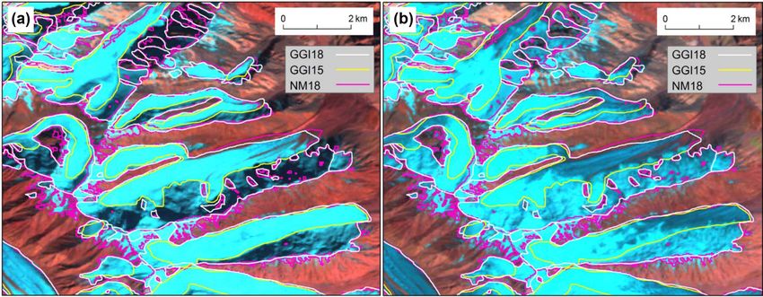
Figure 2. Comparison of glacier outlines used in the GGI15, GGI18, and NM18 inventories at 38.9236◦ N, 72.4217◦ E (path 151, row 33
of WRS2). Backgrounds are false-colour (bands 7, 4, and 2 as RGB) composite Landsat images taken on 28 September 2001 (a) and
26 July 2001 (b). Glacier outlines of the GGI15 (yellow lines) were delineated based on the strongly shaded image on the left, whereas those
of the GGI18 (white lines) were delineated using the less-shaded image on the right. Glacier outlines of the NM18 (pink lines; Mölg et al.,
2018) are also shown for comparison.
eated using multiple images were shown in Fig. S13. There- 1. GAMDAM glacier inventory for high-mountain
fore, the number of images in Fig. 1 represents the degree of Asia: Area–altitude distribution for Central Asia,
delineation accuracy. https://doi.org/10.1594/PANGAEA.891415 (Sakai, 2018a).
As satellite imagery that is cloud-free and has the least 2. GAMDAM glacier inventory for high-mountain
seasonal snow becomes available from existing sources other Asia: Area–altitude distribution for North Asia,
than Landsat in the future, the glacier outlines delineated here https://doi.org/10.1594/PANGAEA.891416 (Sakai, 2018b).
from multiple images need to be revisited and, if necessary, 3. GAMDAM glacier inventory for high-mountain
revised. Sentinel-2 imagery, for instance, might prove a suit- Asia: Area–altitude distribution for South Asia East,
able alternative owing to its high resolution and shorter ac- https://doi.org/10.1594/PANGAEA.891417 (Sakai, 2018c).
quisition interval (≤ 5 d) relative to Landsat. 4. GAMDAM glacier inventory for high-mountain
Asia: Area–altitude distribution for South Asia West,
https://doi.org/10.1594/PANGAEA.891418 (Sakai, 2018d).
5. GAMDAM glacier inventory for high-mountain
5 Summary Asia: Central Asia in ArcGIS (shapefile) format,
https://doi.org/10.1594/PANGAEA.891419 (Sakai, 2018e).
The updated version of the GAMDAM glacier inven- 6. GAMDAM glacier inventory for high-mountain
tory, the GGI18, incorporates all of HMA and includes Asia: North Asia in ArcGIS (shapefile) format,
134 770 glaciers covering 100 693 ± 11 790 km2 . Although https://doi.org/10.1594/PANGAEA.891420 (Sakai, 2018f).
nearly 95 % of the total glacier area was delineated from 7. GAMDAM glacier inventory for high-mountain
summer images, the acquisition date of source imagery Asia: South Asia East in ArcGIS (shapefile) format,
varies widely. Relative to its predecessor (GGI15), the total https://doi.org/10.1594/PANGAEA.891421 (Sakai, 2018g).
glaciated area in HMA is ∼ 15 % greater in the GGI18, due 8. GAMDAM glacier inventory for high-mountain
primarily to the inclusion of glaciated north-facing slopes. Asia: South Asia West in ArcGIS (shapefile) format,
Owing to cloud, seasonal snow cover, and topographic shad- https://doi.org/10.1594/PANGAEA.891422 (Sakai, 2018h).
ing, a number of path–row scenes required multiple Land-
sat images to delineate glacier outlines fully and thus should
be revisited in the future as higher-quality imagery becomes Supplement. The supplement related to this article is available
available. online at: https://doi.org/10.5194/tc-13-2043-2019-supplement.
Data availability. Data can be downloaded from the following Competing interests. The author declares that there is no conflict of
sources. interest.
www.the-cryosphere.net/13/2043/2019/ The Cryosphere, 13, 2043–2049, 20192048 A. Sakai: Updated GAMDAM glacier inventory over high-mountain Asia
Acknowledgements. This project was supported by a grant from the Trouve, E.: Twenty-first century glacier slowdown driven by
Grants-in-Aid for Scientific Research (26257202) of the Japan So- mass loss in High Mountain Asia, Nat. Geosci., 12, 22–27,
ciety for the Promotion of Science. I wish to thank all members of https://doi.org/10.1038/s41561-018-0271-9, 2019.
the GAMDAM project for their valuable support in producing the Farinotti, D., Huss, M., Fürst, J. J., Landmann, J., Machguth, H.,
first version of the GAMDAM glacier inventory. Maussion, F., and Pandit, A.: A consensus estimate for the ice
thickness distribution of all glaciers on Earth, Nat. Geosci., 12,
168–173, 2019.
Financial support. This research has been supported by the Fund- Frey, H., Paul, F., and Strozzi, T.: Compilation of a glacier inven-
ing Program for Next Generation World-Leading Researchers tory for the western Himalayas from satellite data: Methods,
(grant no. GR052). challenges, and results, Remote Sens. Environ., 124, 832–843,
https://doi.org/10.1016/j.rse.2012.06.020, 2012.
Frey, H., Machguth, H., Huss, M., Huggel, C., Bajracharya, S.,
Review statement. This paper was edited by Tobias Bolch and re- Bolch, T., Kulkarni, A., Linsbauer, A., Salzmann, N., and Stof-
viewed by Frank Paul and Wanqin Guo. fel, M.: Estimating the volume of glaciers in the Himalayan–
Karakoram region using different methods, The Cryosphere, 8,
2313–2333, https://doi.org/10.5194/tc-8-2313-2014, 2014.
Gardner, A. S., Moholdt, G., Cogley, J. G., Wouters, B., Arendt,
References A. A., Wahr, J., Berthier, E., Hock, R., Pfeffer, W. T., Kaser, G.,
Ligtenberg, S. R. M., Bolch, T., Sharp, M. J., Hagen, J. O., van
Arendt, A., Bliss, A., Bolch, T., Cogley, J. G., Gardner, A. S., den Broeke, M. R., and Paul, F.: A reconciled estimate of glacier
Hagen, J.-O., Hock, R., Huss, M., Kaser, G., Kienholz, C., Pf- contributions to sea level rise: 2003 to 2009, Science, 340, 852–
effer, W. T., Moholdt, G., Paul, F., Radić, V., Andreassen, L. 857, https://doi.org/10.1126/science.1234532, 2013.
M., Bajracharya, S., Barrand, N. E., Beedle, M., Berthier, E., Guo, W., Liu, S., Xu, J., Wu, L., Shangguan, D., Yao, X., Wei,
Bhambri, R., Brown, I., Burgess, E. W., Burgess, D., Cawk- J., Bao, W., Yu, P., Liu, Q., and Jiang, Z.: The second Chinese
well, F., Chinn, T., Copland, L., Davies, B., Angelis, H. de, glacier inventory: Data, methods and results, J. Glaciol., 61, 357–
Dolgova, E., Earl, L., Filbert, K., Forester, R., Fountain, A. G., 372, https://doi.org/10.3189/2015JoG14J209, 2015.
Frey, H., Giffen, B., Glasser, N. F., Guo, W., Gurney, S. D., Herreid, S., Pellicciotti, F., Ayala, A., Chesnokova, A., Kienholz,
Hagg, W., Hall, D., Haritashya, U. K., Hartmann, G., Helm, C., C., Shea, J., and Shrestha, A.: Satellite observations show no net
Herreid, S., Howat, I., Kapustin, G., Khromova, T. E., König, change in the percentage of supraglacial debris-covered area in
M., Kohler, J., Kriegel, D., Kutuzov, S., Lavrentiev, I., Le Bris, northern Pakistan from 1977 to 2014, J. Glaciol., 61, 524–536,
R., Liu, S., Lund, J., Manley, W., Marti, R., Mayer, C., Miles, https://doi.org/10.3189/2015JoG14J227, 2015.
E. S., Li, X., Menounos, B., Mercer, A., Mölg, N., Mool, P., Huss, M. and Hock, R.: A new model for global glacier
Nosenko, G., Negrete, A., Nuimura, T., Nuth, C., Pettersson, change and sea-level rise, Front. Earth Sci., 3, 54,
R., Racoviteanu, A., Ranzi, R., Rastner, P., Rau, F., Raup, B., https://doi.org/10.3389/feart.2015.00054, 2015.
Rich, J., Rott, H., Sakai, A., Schneider, C., Seliverstov, Y., Sharp, Immerzeel, W. W., van Beek, L. P. H., and Bierkens, M. F. P.: Cli-
M. J., Sigurðsson, O., Stokes, C. R., Way, R. G., Wheate, R., mate change will affect the Asian water towers, Science, 328,
Winsvold, S., Wolken, G., Wyatt, F., and Zheltihyna, N.: Ran- 1382–1385, https://doi.org/10.1126/science.1183188, 2010.
dolph Glacier Inventory – A Dataset of Global Glacier Outlines: Kääb, A., Berthier, E., Nuth, C., Gardelle, J., and Arnaud,
Version 5.0: GLIMS Technical Report, Global Land Ice Mea- Y.: Contrasting patterns of early twenty-first century glacier
surement from Space, Colorado, USA, Digital Media, available mass change in the Himalayas, Nature, 488, 495–498,
at: http://www.glims.org/RGI/randolph50.html (last access: 17 https://doi.org/10.1038/nature11324, 2012.
July 2019), 2015. Kääb, A., Treichler, D., Nuth, C., and Berthier, E.: Brief Communi-
Bodin, X., Rojas, F., and Brenning, A.: Status and cation: Contending estimates of 2003–2008 glacier mass balance
evolution of the cryosphere in the Andes of Santi- over the Pamir–Karakoram–Himalaya, The Cryosphere, 9, 557–
ago (Chile, 33.5◦ S), Geomorphology, 118, 453–464, 564, https://doi.org/10.5194/tc-9-557-2015, 2015.
https://doi.org/10.1016/j.geomorph.2010.02.016, 2010. Marzeion, B., Kaser, G., Maussion, F., and Champollion, N.:
Bolch, T., Kulkarni, A., Kaab, A., Huggel, C., Paul, F., Cogley, J. G., Limited influence of climate change mitigation on short-
Frey, H., Kargel, J. S., Fujita, K., Scheel, M., Bajracharya, S., and term glacier mass loss, Nat. Clim. Change, 8, 305–308,
Stoffel, M.: The state and fate of Himalayan glaciers, Science, https://doi.org/10.1038/s41558-018-0093-1, 2018.
336, 310–314, https://doi.org/10.1126/science.1215828, 2012. Minora, U., Bocchiola, D., D’Agata, C., Maragno, D., Mayer,
Bolch, T., Pieczonka, T., Mukherjee, K., and Shea, J.: Brief com- C., Lambrecht, A., Vuillermoz, E., Senese, A., Compostella,
munication: Glaciers in the Hunza catchment (Karakoram) have C., Smiraglia, C., and Diolaiuti, G. A.: Glacier area
been nearly in balance since the 1970s, The Cryosphere, 11, 531– stability in the Central Karakoram National Park (Pak-
539, https://doi.org/10.5194/tc-11-531-2017, 2017. istan) in 2001–2010, Prog. Phys. Geog., 40, 629–660,
Brun, F., Berthier, E., Wagnon, P., Kääb, A., and Treichler, https://doi.org/10.1177/0309133316643926, 2016.
D.: A spatially resolved estimate of High Mountain Asia Mölg, N., Bolch, T., Rastner, P., Strozzi, T., and Paul, F.: A
glacier mass balances, 2000–2016, Nat. Geosci., 10, 668–673, consistent glacier inventory for Karakoram and Pamir de-
https://doi.org/10.1038/NGEO2999, 2017. rived from Landsat data: distribution of debris cover and
Dehecq, A., Gourmelen, N., Gardner, A. S., Brun, F., Goldberg.,
D., Neinow P. W., Berthier, E., Vincent, C., Wagnon, P., and
The Cryosphere, 13, 2043–2049, 2019 www.the-cryosphere.net/13/2043/2019/A. Sakai: Updated GAMDAM glacier inventory over high-mountain Asia 2049 mapping challenges, Earth Syst. Sci. Data, 10, 1807–1827, RGI Consortium: Randolph Glacier Inventory 6.0, available at: https://doi.org/10.5194/essd-10-1807-2018, 2018. https://www.glims.org/RGI/ (last access: 17 July 2019), 2017. Naegeli, K., Huss, M., and Hoelzle, M.: Change detection of bare- Sakai, A.: GAMDAM glacier inventory for High Moun- ice albedo in the Swiss Alps, The Cryosphere, 13, 397–412, tain Asia: Area–altitude distribution for Central Asia, https://doi.org/10.5194/tc-13-397-2019, 2019. https://doi.org/10.1594/PANGAEA.891415, 2018a. Nagai, H., Fujita, K., Sakai, A., Nuimura, T., and Tadono, T.: Com- Sakai, A.: GAMDAM glacier inventory for High Moun- parison of multiple glacier inventories with a new inventory de- tain Asia: Area–altitude distribution for North Asia, rived from high-resolution ALOS imagery in the Bhutan Hi- https://doi.org/10.1594/PANGAEA.891416, 2018b. malaya, The Cryosphere, 10, 65–85, https://doi.org/10.5194/tc- Sakai, A.: GAMDAM glacier inventory for High Moun- 10-65-2016, 2016. tain Asia: Area–altitude distribution for South Asia East, Nuimura, T., Fujita, K., Yamaguchi, S., and Sharma, R. R.: Ele- https://doi.org/10.1594/PANGAEA.891417, 2018c. vation changes of glaciers revealed by multitemporal digital el- Sakai, A.: GAMDAM glacier inventory for High Moun- evation models calibrated by GPS survey in the Khumbu re- tain Asia: Area–altitude distribution for South Asia West, gion, Nepal Himalaya, 1992–2008, J. Glaciol., 58, 648–656, https://doi.org/10.1594/PANGAEA.891418, 2018d. https://doi.org/10.3189/2012JoG11J061, 2012. Sakai, A.: GAMDAM glacier inventory for High Moun- Nuimura, T., Sakai, A., Taniguchi, K., Nagai, H., Lamsal, D., tain Asia: Central Asia in ArcGIS (shapefile) format, Tsutaki, S., Kozawa, A., Hoshina, Y., Takenaka, S., Omiya, https://doi.org/10.1594/PANGAEA.891419, 2018e. S., Tsunematsu, K., Tshering, P., and Fujita, K.: The GAM- Sakai, A.: GAMDAM glacier inventory for High Moun- DAM glacier inventory: a quality-controlled inventory of Asian tain Asia: North Asia in ArcGIS (shapefile) format, glaciers, The Cryosphere, 9, 849–864, https://doi.org/10.5194/tc- https://doi.org/10.1594/PANGAEA.891420, 2018f. 9-849-2015, 2015. Sakai, A.: GAMDAM glacier inventory for High Moun- Ojha, S., Fujita, K., Sakai, A., Nagai, H., and Lamsal, D.: tain Asia: South Asia East in ArcGIS (shapefile) format, Topographic controls on the debris-cover extent of glaciers https://doi.org/10.1594/PANGAEA.891421, 2018g. in the Eastern Himalayas: Regional analysis using a novel Sakai, A.: GAMDAM glacier inventory for High Moun- high-resolution glacier inventory, Quatern. Int., 455, 82–92, tain Asia: South Asia West in ArcGIS (shapefile) format, https://doi.org/10.1016/j.quaint.2017.08.007, 2017. https://doi.org/10.1594/PANGAEA.891422, 2018h. Paul, F., Kääb, A., Maisch, M., Kellenberger, T., and Hae- Sakai, A. and Fujita, K.: Contrasting glacier responses to recent berli, W.: The new remote-sensing-derived Swiss glacier climate change in high-mountain Asia, Sci. Rep., 7, 13717, inventory: I. Methods, Ann. Glaciol., 34, 355–361, https://doi.org/10.1038/s41598-017-14256-5, 2017. https://doi.org/10.3189/172756402781817941, 2002. Shannon, S., Smith, R., Wiltshire, A., Payne, T., Huss, M., Betts, Radić, V. and Hock, R.: Glaciers in the Earth’s hydrologi- R., Caesar, J., Koutroulis, A., Jones, D., and Harrison, S.: Global cal cycle: Assessments of glacier mass and runoff changes glacier volume projections under high-end climate change sce- on global and regional scales, Surv. Geophys., 3, 1–25, narios, The Cryosphere, 13, 325–350, https://doi.org/10.5194/tc- https://doi.org/10.1007/s10712-013-9262-y, 2013. 13-325-2019, 2019. www.the-cryosphere.net/13/2043/2019/ The Cryosphere, 13, 2043–2049, 2019
You can also read