CONTINUAL LEARNING USING HASH-ROUTED CONVO-LUTIONAL NEURAL NETWORKS
←
→
Page content transcription
If your browser does not render page correctly, please read the page content below
Under review as a conference paper at ICLR 2021

C ONTINUAL LEARNING USING HASH - ROUTED CONVO -
LUTIONAL NEURAL NETWORKS

 Anonymous authors
 Paper under double-blind review

                                           A BSTRACT

         Continual learning could shift the machine learning paradigm from data centric
         to model centric. A continual learning model needs to scale efficiently to handle
         semantically different datasets, while avoiding unnecessary growth. We introduce
         hash-routed convolutional neural networks: a group of convolutional units where
         data flows dynamically. Feature maps are compared using feature hashing and
         similar data is routed to the same units. A hash-routed network provides excellent
         plasticity thanks to its routed nature, while generating stable features through the
         use of orthogonal feature hashing. Each unit evolves separately and new units
         can be added (to be used only when necessary). Hash-routed networks achieve
         excellent performance across a variety of typical continual learning benchmarks
         without storing raw data and train using only gradient descent. Besides providing
         a continual learning framework for supervised tasks with encouraging results, our
         model can be used for unsupervised or reinforcement learning.

1   I NTRODUCTION

When faced with a new modeling challenge, a data scientist will typically train a model from a class
of models based on her/his expert knowledge and retain the best performing one. The trained model
is often useless when faced with different data. Retraining it on new data will result in poor perfor-
mance when trying to reuse the model on the original data. This is what is known as catastrophic
forgetting (McCloskey & Cohen, 1989). Although transfer learning avoids retraining networks from
scratch, keeping the acquired knowledge in a trained model and using it to learn new tasks is not
straightforward. The real knowledge remains with the human expert. Model training is usually a
data centric task. Continual learning (Thrun, 1995) makes model training a model centric task by
maintaining acquired knowledge in previous learning tasks.
Recent work in continual (or lifelong) learning has focused on supervised classification tasks and
most of the developed algorithms do not generate stable features that could be used for unsupervised
learning tasks, as would a more generic algorithm such as the one we present. Models should also
be able to adapt and scale reasonably to accommodate different learning tasks without using an ex-
ponential amount of resources, and preferably with little data scientist intervention.
To tackle this challenge, we introduce hash-routed networks (HRN). A HRN is composed of mul-
tiple independent processing units. Unlike typical convolutional neural networks (CNN), the data
flow between these units is determined dynamically by measuring similarity between hashed feature
maps. The generated feature maps are stable. Scalability is insured through unit evolution and by
increasing the number of available units, while avoiding exponential memory use.
This new type of network maintains stable performance across a variety of tasks (including seman-
tically different tasks). We describe expansion, update and regularization algorithms for continual
learning. We validate our approach using multiple publicly available datasets, by comparing super-
vised classification performance. Benchmarks include Pairwise-MNIST, MNIST/Fashion-MNIST
(Xiao et al., 2017) and SVHN/incremental-Cifar100 (Netzer et al., 2011; Krizhevsky et al., 2009).
Relevant background is introduced in section 2. Section 3 details the hash-routing algorithm and
discusses its key attributes. Section 4 compares our work with other continual learning and dynamic
network studies. A large set of experiments is carried out in section 5.

                                                  1
Under review as a conference paper at ICLR 2021

2     F EATURE HASHING BACKGROUND
Feature hashing, also known as the hashing trick (Weinberger et al., 2009) is a dimension
reduction transformation with key properties for our work: inner product conservation and
quasi-orthogonality. A feature hashing function φ : RN → Rs , can be built using two uniform hash
functions h : N → {1, 2..., s} and ξ : N → {−1, 1}, as such:
                                                X
                                       φi (x) =       ξ(j)xj
                                                  j∈[[1,N ]]
                                                  j:h(j)=i

where φi denotes the ith component of φ. Inner product is preserved as E[φ(a)T φ(b)] = aT b. φ
provides an unbiased estimator of the inner product. It can also be shown that if ||a||2 = ||b||2 = 1,
then σa,b = O( 1s ).
Two different hash functions φ and φ0 (e.g. h 6= h0 or ξ 6= ξ 0 ) are orthogonal. In other words,
∀(v, w) ∈ Im(φ) × Im(φ0 ), E[vT w] ≈ 0. Furthermore, Weinberger et al. (2009) details the inner
product bounds, given v ∈ Im(φ) and x ∈ RN :
                                                                                     !
                     T 0                                         2 /2
              P r(|v φ (x)| > ) ≤ 2 exp −               2     2                                   (1)
                                                s−1 kvk2 kxk2 + kvk∞ kxk∞ /3
Eq.1 shows that approximate orthogonality is better when φ0 handles bounded vectors. Data inde-
                                                                            v
pendent bounds can be obtained by setting kxk∞ = 1 and replacing v by kvk      , which leads to
                                                                                      2
      2
kxk2 ≤ N and kvk∞ ≤ 1, hence:
                                                                    !
                                                     2 /2                            2 /2

                 T   0
           P r(|v φ (x)| > ) ≤ 2 exp −              2                  ≤ 2 exp −                     (2)
                                            s−1 kxk2 + kvk∞ /3                     N/s + /3
Better approximate orthogonality significantly reduces correlation when summing feature vectors
generated by different hashing functions, as is done in hash-routed networks.

3     H ASH - ROUTED NETWORKS
3.1       S TRUCTURE

A hash-routed network maps input data to a feature vector of size s that is stable across successive
learning tasks. An HRN exploits inner product preservation to insure that similarity between gen-
erated feature vectors reflect the similarity between input samples. Quasi-orthogonality of different
feature hashing functions is used to reduce correlation between the output’s components, as it is the
sum of individual hashed feature vectors. An HRN H is composed of M units {U1 , ..., UM }. Each
unit Uk is composed of:
          • A series of convolution operations fk . It is characterized by a number of input channels
            and a number of output channels, resulting in a vector of trainable parameters wk . Note
            that fk can also include pooling operations.
          • An orthonormal projection basis Bk . It contains a maximum of m non-zeros orthogonal
            vectors of size s. Each basis is filled with zero vectors at first. These will be replaced by
            non-zero vectors during training.
          • A feature hashing function φk that maps a feature vector of any size to a vector of size s.
The network also has an independent feature hashing function φ0 . All the feature hashing functions
are different but generate feature vectors of size s.

3.2       O PERATION

3.2.1      H ASH - ROUTING ALGORITHM
H maps an input sample x to a feature vector H(x) of size s. In a vanilla CNN, x would go through
a series of deterministic convolutional layers to generate feature maps of growing size. In a HRN,

                                                     2
Under review as a conference paper at ICLR 2021

Figure 1: A hash-routed network with 4 units and a depth of 3. In this example, U3 is selected first as
the hashed flattened image has the highest projection (p0 ) magnitude onto its basis. The structured
image passes through the unit’s convolution filters, generating the feature map in the middle. This
process is repeated twice whilst disregarding used units at each level. The final output is the sum of
all projection residues. Best viewed in color.

the convolutional layers that will be involved will vary depending on intermediate results.
Feature hashing is used to route operations. Since feature hashing preserves the inner product in the
hashed features space, similar samples will be processed similarly. Intermediate features are hashed
and projected upon the units’ projection bases. The unit where the projection’s magnitude is the
highest is selected for the next operation. Operations continue until a maximum depth d is reached
(i.e. there is a limit of d − 1 chained operations), or when the projection residue is below a given
threshold τd . H(x) is the sum of all residues.
Let {Ui1 , Ui2 , ..., Uid−1 } be the ordered set of units involved in processing x (assuming the final pro-
jection residue’s magnitude is greater than τd ). Operation 0 simply involves hashing the (flattened)
input sample using φ0 . Let xik = fik ◦ fik−1 ◦ ... ◦ fi1 (x) be the intermediate features obtained at
operation k. The normalized hashed features vector after operation k is computed as such:

                                                              xik
                                                    φ ik
                                                           kxik k∞
                                          hik =                                                       (3)
                                                             xik
                                                   φ ik
                                                           kxik k∞ 2
For operation 0, hi0 is computed using x and φ0 .
pik = Bik+1 hik and rik = hik − pik are the projection vector and residue vector over basis Bik+1
resp. As explained earlier, this means that:
                                    ik+1 =     arg max           kBj hik k2                            (4)
                                             j∈I\{i1 ,...,ik }

where I is the subset of initialized units (i.e. units with bases containing at least one non-zero
vector). Finally,                                  X
                                     H(x) =                 rj                                 (5)
                                                  j∈{i0 ,...,id−1 }

The full inference algorithm is summarized in Algorithm 1 and an example is given in Figure 1.

3.2.2   A NALYSIS
The output of a typical CNN is a feature map with a dimension that depends on the number of
output channels used in each convolutional layer. In a HRN, this would lead to a variable dimension
output as the final feature map depends on the routing. In a continual learning setup, dealing with
variable dimension feature maps would be impractical. Feature hashing circumvents these problems
by generating feature vectors of fixed dimension.
Similar feature maps get to be processed by the same units, as a consequence of using feature hashing

                                                      3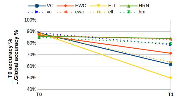
Under review as a conference paper at ICLR 2021

Algorithm 1: Hash-routed inference
Input: x
Output: H = H(x)
h0 = φ0 (x); J = ∅
H ← 0; h ← h0 ; y ← x
for j = 1, ..., d − 1 do
    ij = arg maxk∈I\J kBk hk2 ;
       // select the best unit
      r ← h − Bij h ;        // compute new residue
      H ←H +r;               // accumulate residue for output
      J ← J ∪ {ij } ;        // update set of used units
      if krk2 < τd then
          break ;                           // stop processing when residue is too low
      else
          y ← fij (y) ;                     // compute feature map
                        y
                φij ( kyk       )
         h←             y
                            ∞
                                        ;   // new hash vector using flattened feature map
                φij ( kyk   )
                        ∞           2
   end
end

for routing. In this context, similarity is measured by the inner product of flattened feature maps,
projected onto different orthogonal subspaces (each unit basis span). Another consequence is that
unit weights become specialized in processing a certain type of features, rather than having to adapt
to task specific features. This provides the kind of stability needed for continual learning.
For a given unit Uk , rank(Bk ) ≤ m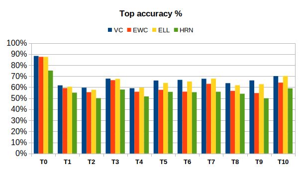
Under review as a conference paper at ICLR 2021

3.3.2    U PDATE
Once a unit basis is full (i.e. it does not contain any zero vector), it still needs to evolve to accommo-
date routing needs. As the network trains, hashed features will also change and routing might need
adjustment. If nothing is done to update full basis, the network might get ”stuck” in a bad config-
uration. Network weights would then need to change in order to compensate for improper routing,
resulting in a decrease in performance. Nevertheless, bases should not be updated too frequently
as this would lead to instability and units would then need to learn to deal with too many routing
configurations.
An aging mechanism can be used to stabilize basis update as training progresses. Each time a unit
is selected, a counter is incremented and when it reaches its maximum age, it is updated. The maxi-
mum age can then be increased by means of a geometric progression.
Using the aging mechanism, it becomes possible to apply the update process to bases that are not yet
full, thus adding more flexibility. Hence, some bases can expand to include new vectors and update
existing ones.
Bases can be updated by replacing vectors that lead to routing instability. Each non-zero basis vector
vk has a low projection counter ck . During training, when a unit has been selected, the basis vec-
tor with the lowest projection magnitude sees its low projection counter incremented. The update
algorithm is summarized in Algorithm 2.

Algorithm 2: Unit update
Input: Current basis (excluding zero-vectors): B = (v1 , ..., vm ),
Current low projection counters: (c1 , ..., cm ),
Current age: a, Current maximum age: α, Aging rate: ρ > 1,
Latest hash vector h
Output: Updated basis
if a = α then
     i = arg max{cj };            // find basis vector to replace
     vi ← h − B−i h;              // remove projection on the reduced basis B−i
                                         (without vi )
    vi ← kvviik
                2
    α ← ρα;                         // update maximum age
    a ← 0;                          // reset age counter
    ci ← 0;                         // reset low projection counter
else
    a ← a + 1;                      // increment current age
    i = arg min vjT h    2
                           ;        // find low projection counter to increment
    ci ← ci + 1

3.4     T RAINING AND SCALABILITY

HRNs generate feature vectors that can be used for a variety of learning tasks. Given a learning task,
optimal network weights can be computed via gradient descent. Feature vectors can be used as input
to a fully connected network, to match a given label distribution in the case of supervised learning.
As explained in Algorithm 1, each input sample is processed differently and can lead to a different
computation graph. Batching is still possible and weight updates only apply to units involved in
processing batch data. Weight updates is regularized using the residue vector’s norm at each unit
level. Low magnitude residue vectors have little contribution to the network’s output thus their
impact on training of downstream units should be limited. Denoting L a learning task loss function,
r the hash vector projection residue over a unit’s basis, w the vector of the unit’s trainable weights
and γ a learning rate, regularized weight update of w becomes:
                                  w ← w − γ min(1, krk2 )∇L(w)                                     (7)
An HRN can scale simply by adding extra units. Note that adding units between each learning task
is not always necessary to insure optimal performance. In our experiments, units were manually
added after some learning tasks but this expansion process could be made automatic. Indeed, one or
more extra unit(s) could be automatically added whenever all bases have been completely filled. Its
architecture could be a copy of an existing unit (chosen randomly).

                                                    5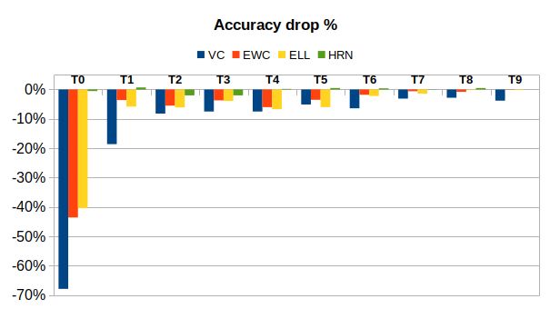
Under review as a conference paper at ICLR 2021

4     R ELATED WORK

Dynamic networks Using handcrafted rigid models has obvious limits in terms of scalability.
Tanno et al. (2018) builds a binary tree CNN with a routed dataflow. Routing heuristics requires
intermediate evaluation on training data. It uses fully connected layers to select a branch. Spring &
Shrivastava (2017) builds LSH (Gionis et al., 1999) hash tables of fully connected layer weights to
select relevant activations but this does not apply to CNN. Rosenbaum et al. (2017)’s algorithm is
closer to our setup. Each sample is processed by different blocks until a maximum processing depth
is reached. It uses reinforcement learning to train a router that selects the best processing block at
each level, based on a supervised classification scheme. However, their network is task-aware and
blocks at each level cannot be used at other levels (unlike HRN units).

Continual learning Parisi et al. (2019) offers a thorough review of state-of-the-art continual learn-
ing techniques and algorithms, insisting on a key trade-off: stability vs plasticity. Lomonaco &
Maltoni (2017) groups continual learning algorithms into 3 categories: regularization, architectural
and rehearsal. Kirkpatrick et al. (2017) introduces a regularization technique using the Fisher in-
formation matrix to avoid updating important network weights. Zenke et al. (2017) achieves the
same goal by measuring weight importance through its contribution to overall loss evolution across
a given number of updates. Rannen et al. (2017) is closer to our setup. The authors continuously
train an encoder with different decoders for each task while keeping a stable feature map. Knowl-
edge distillation (Hinton et al., 2015) is used to avoid significant changes to the generated features
between each task. A key limitation of this technique is, as mentioned in Rannen et al. (2017), that
the encoder will never evolve beyond its inherent capacity as its architecture is frozen. Serra et al.
(2018) learns attention nearly-binary masks to avoid updating parts of the network when training
for a new task. Similarly, Beaulieu et al. (2020) uses a primary model to modulate the update and
response of a secondary model. In both cases, scalability is again limited by the chosen architecture.
Li & Hoiem (2017) also uses knowledge distillation in a supervised learning setup but systemati-
cally enlarges the last layers to handle new classes. Yoon et al. (2017) limits network expansion by
enforcing sparsity when training with extra neurons. Useless neurons are then removed. Xu & Zhu
(2018) uses reinforcement learning to optimize network expansion but does not fully take advantage
of the inherent network capacity as network weights are frozen before each new task.
Lopez-Paz & Ranzato (2017); Rebuffi et al. (2017); Hayes et al. (2019) store data from previous
tasks in various ways to be reused during the current task (rehearsal). Shin et al. (2017); van de
Ven & Tolias (2018); Rios & Itti (2018) make use of generative networks to regenerate data from
previous tasks. Kamra et al. (2017); Parisi et al. (2018); Kemker & Kanan (2017) use neuroscience
inspired concepts such as short-term/long-term memories and a fear mechanism to selectively store
data during learning tasks, whereas we store a limited number of hashed feature maps in each unit
basis, updated using an aging mechanism.

5     E XPERIMENTS

5.1   S ETUP

We test our approach in scenarios of increasing complexity and using semantically different datasets.
Supervised classification scenarios involve a single HRN that is used across all tasks to generate a
feature vector that is fed to different classifiers (one classifier per task). Each classifier is trained
only during the task at hand, along with the common HRN. Once the HRN has finished training for
a given task, test data from previous tasks is re-encoded using the latest version of the HRN. The
new feature vectors are fed into the trained (and frozen) classifiers and accuracy for previous tasks
is measured once more.
We compare our approach against 3 other algorithms: a vanilla convolutional network (VC) for fea-
ture generation with a different classifier per task; Elastic Weight Consolidation (EWC) (Kirkpatrick
et al., 2017), a typical benchmark for continual learning. Elastic weight consolidation is applied only
to a feature generator that feeds into a different classifier per task; Encoder Based Lifelong learning
(ELL) (Rannen et al., 2017), involving a common feature generator with a different classifier per
task. For a fair comparison, we used the same number of epochs per task and the same architecture
for classifiers and convolutional layers. For VC, EWC and ELL, the convolutional encoder is equiv-
alent to the unit combination in HRN leading to the largest feature map. Feature codes used in ELL

                                                   6
Under review as a conference paper at ICLR 2021
autoencoders (see Rannen et al. (2017) for more detail) have the same size as the hashed-feature
vectors in HRN. For all experiments, we show the evolution of accuracy for the first task (T0) after
each task training. This is a clear measure of catastrophic forgetting. We also show the overall
accuracy after each task training.
The following scenarios were considered (implementation details can be found in Appendix.C):
Pairwise-MNIST Each task is a binary classification of handwritten digits: 0/1, 2/3, ...etc, for a total
of 5 tasks (5 epochs each). In this case, tasks are semantically comparable. A 4 units HRN with a
depth of 3 was used.
MNIST/Fashion-MNIST There are two 10-classes supervised classification tasks, first the Fashion-
MNIST dataset, then the MNIST dataset. This a 2 tasks scenario with semantically different datasets.
A 6 units HRN (depth of 3) was used for the first task and 2 units were added for the second task.
SVHN/incremental-Cifar100 This is an 11 tasks scenario, where each task is a 10-classes super-
vised classification. Task 0 (8 epochs) involves the SVHN dataset. Tasks 1 to 10 (15 epochs each),
involve 10 classes out of the 100 classes available in the Cifar100 dataset (new classes are intro-
duced incrementally by groups of 10). All datasets are semantically different, especially task 0 and
the others. A HRN of 6 units (depth of 3) was used for the SVHN task and 2 extra units were added
before the 10 Cifar100 tasks series. For this experiment, we provide the accuracy drop for each task
between its first training and the final task. This is a clear measure of catastrophic forgetting. We
also provide the top accuracy score for each task. This measures the network’s ability to learn new
tasks.
Figure 2: Task 0 accuracy evaluation after each task (continous lines) and global accuracy score
(dotted lines). Top: SVHN/incremental-Cifar100. Bottom-left: Pairwise-MNIST. Bottom-right:
MNIST/Fashion-MNIST. Best viewed in color.
5.2 C OMPARATIVE ANALYSIS
Figure 2 shows that HRN maintains a stable performance for the initial task, in comparison to other
techniques, even in the most complex scenario. Global accuracy plots show that HRN performance
degradation for all tasks is very low (even slightly positive in some cases). Moreover, figure 3 shows
that catastrophic forgetting is higher with other algorithms, and almost non-existent with HRN.
However, 3 also shows that maximum accuracy for each task is often slightly lower in comparison
to other algorithms. Indeed, units in a HRN are not systematically updated at each training step and
7Under review as a conference paper at ICLR 2021
Figure 3: SVHN/incremental-Cifar100. Top: Final accuracy drop for each task. Bottom: Top
accuracy score for each task. Best viewed in color.
would hence, require a few more epochs to reach top task accuracy as with VC. Furthermore, the
trade-off between plasticity and stability can be controlled through the λ parameter (see Eq.6) as the
ablation study has shown (see B for more detail). Plasticity can also be increased by adding extra
units to an HRN.
5.3 ROUTING AND NETWORK ANALYSIS
After a few epochs, we observe that some units are used more frequently than others. However, we
observe significant changes in usage ratios especially when changing tasks and datasets (see Figure
4). This clearly shows the network’s adaptability when dealing with new data. Moreover, some units
are almost never used (e.g. U6 in Figure 4). This shows that the HRN only uses what it needs and
that adding extra units does not necessarily lead to better performance.
Figure 4: HRN units relative usage ratios for the SVHN/incremental-Cifar100 scenario. Units 6 and
7 were added after T0 (SVHN). Best viewed in color.
8Under review as a conference paper at ICLR 2021
5.4 H YPERPARAMETERS AND ABLATION
Appendix B details the impact of key hyperparameters. Most importantly, the `1 -norm constraint
over the residue vectors (see Eq.6) plays a crucial role in keeping long-term performance but slightly
reduces short-term performance. This can be compensated by increasing the number of epochs per
task. We have also considered keeping the projection vectors in the output of HRN (the output
would be the sum of projection vectors concatenated with the sum of residue vectors) but we saw no
significant impact on performance.
6 C ONCLUSION AND FUTURE WORK
We have introduced the use of feature hashing to generate dynamic configurations in modular convo-
lutional neural networks. Hash-routed convolutional networks generate stable features that exhibit
excellent stability and plasticity across a variety of semantically different datasets. Results show
excellent feature generation stability, surpassing typical and comparable continual learning bench-
marks. Continual supervised learning using HRN still involves the use of different classifiers, even
though compression techniques (such as (Chen et al., 2015)) can reduce required memory. This
limitation is also a design choice, as it does not limit the use of HRN to supervised classification.
Future work will explore the use of HRN in unsupervised and reinforcement learning setups.
R EFERENCES
Shawn Beaulieu, Lapo Frati, Thomas Miconi, Joel Lehman, Kenneth O Stanley, Jeff Clune, and
Nick Cheney. Learning to continually learn. arXiv preprint arXiv:2002.09571, 2020.
Wenlin Chen, James Wilson, Stephen Tyree, Kilian Weinberger, and Yixin Chen. Compressing
neural networks with the hashing trick. In International conference on machine learning, pp.
2285–2294, 2015.
Aristides Gionis, Piotr Indyk, Rajeev Motwani, et al. Similarity search in high dimensions via
hashing. In Vldb, volume 99, pp. 518–529, 1999.
Tyler L Hayes, Nathan D Cahill, and Christopher Kanan. Memory efficient experience replay for
streaming learning. In 2019 International Conference on Robotics and Automation (ICRA), pp.
9769–9776. IEEE, 2019.
Geoffrey Hinton, Oriol Vinyals, and Jeff Dean. Distilling the knowledge in a neural network. arXiv
preprint arXiv:1503.02531, 2015.
Nitin Kamra, Umang Gupta, and Yan Liu. Deep generative dual memory network for continual
learning. arXiv preprint arXiv:1710.10368, 2017.
Ronald Kemker and Christopher Kanan. Fearnet: Brain-inspired model for incremental learning.
arXiv preprint arXiv:1711.10563, 2017.
James Kirkpatrick, Razvan Pascanu, Neil Rabinowitz, Joel Veness, Guillaume Desjardins, Andrei A
Rusu, Kieran Milan, John Quan, Tiago Ramalho, Agnieszka Grabska-Barwinska, et al. Overcom-
ing catastrophic forgetting in neural networks. Proceedings of the national academy of sciences,
114(13):3521–3526, 2017.
Alex Krizhevsky, Geoffrey Hinton, et al. Learning multiple layers of features from tiny images.
2009.
Zhizhong Li and Derek Hoiem. Learning without forgetting. IEEE transactions on pattern analysis
and machine intelligence, 40(12):2935–2947, 2017.
Vincenzo Lomonaco and Davide Maltoni. Core50: a new dataset and benchmark for continuous
object recognition. arXiv preprint arXiv:1705.03550, 2017.
David Lopez-Paz and Marc’Aurelio Ranzato. Gradient episodic memory for continual learning. In
Advances in Neural Information Processing Systems, pp. 6467–6476, 2017.
9Under review as a conference paper at ICLR 2021
Michael McCloskey and Neal J Cohen. Catastrophic interference in connectionist networks: The
sequential learning problem. In Psychology of learning and motivation, volume 24, pp. 109–165.
Elsevier, 1989.
Yuval Netzer, Tao Wang, Adam Coates, Alessandro Bissacco, Bo Wu, and Andrew Y Ng. Reading
digits in natural images with unsupervised feature learning. 2011.
German I Parisi, Jun Tani, Cornelius Weber, and Stefan Wermter. Lifelong learning of spatiotempo-
ral representations with dual-memory recurrent self-organization. Frontiers in neurorobotics, 12:
78, 2018.
German I Parisi, Ronald Kemker, Jose L Part, Christopher Kanan, and Stefan Wermter. Continual
lifelong learning with neural networks: A review. Neural Networks, 2019.
Amal Rannen, Rahaf Aljundi, Matthew B Blaschko, and Tinne Tuytelaars. Encoder based lifelong
learning. In Proceedings of the IEEE International Conference on Computer Vision, pp. 1320–
1328, 2017.
Sylvestre-Alvise Rebuffi, Alexander Kolesnikov, Georg Sperl, and Christoph H Lampert. icarl:
Incremental classifier and representation learning. In Proceedings of the IEEE conference on
Computer Vision and Pattern Recognition, pp. 2001–2010, 2017.
Amanda Rios and Laurent Itti. Closed-loop gan for continual learning. CoRR, 2018.
Clemens Rosenbaum, Tim Klinger, and Matthew Riemer. Routing networks: Adaptive selection of
non-linear functions for multi-task learning. arXiv preprint arXiv:1711.01239, 2017.
Joan Serra, Didac Suris, Marius Miron, and Alexandros Karatzoglou. Overcoming catastrophic
forgetting with hard attention to the task. arXiv preprint arXiv:1801.01423, 2018.
Hanul Shin, Jung Kwon Lee, Jaehong Kim, and Jiwon Kim. Continual learning with deep generative
replay. In Advances in Neural Information Processing Systems, pp. 2990–2999, 2017.
Ryan Spring and Anshumali Shrivastava. Scalable and sustainable deep learning via randomized
hashing. In Proceedings of the 23rd ACM SIGKDD International Conference on Knowledge
Discovery and Data Mining, pp. 445–454, 2017.
Ryutaro Tanno, Kai Arulkumaran, Daniel C. Alexander, Antonio Criminisi, and Aditya V. Nori.
Adaptive neural trees. CoRR, abs/1807.06699, 2018. URL http://arxiv.org/abs/
1807.06699.
Sebastian Thrun. A lifelong learning perspective for mobile robot control. In Intelligent Robots and
Systems, pp. 201–214. Elsevier, 1995.
Gido M van de Ven and Andreas S Tolias. Generative replay with feedback connections as a general
strategy for continual learning. arXiv preprint arXiv:1809.10635, 2018.
Kilian Weinberger, Anirban Dasgupta, John Langford, Alex Smola, and Josh Attenberg. Feature
hashing for large scale multitask learning. In Proceedings of the 26th annual international con-
ference on machine learning, pp. 1113–1120, 2009.
Han Xiao, Kashif Rasul, and Roland Vollgraf. Fashion-mnist: a novel image dataset for benchmark-
ing machine learning algorithms, 2017.
Ju Xu and Zhanxing Zhu. Reinforced continual learning. In Advances in Neural Information Pro-
cessing Systems, pp. 899–908, 2018.
Jaehong Yoon, Eunho Yang, Jeongtae Lee, and Sung Ju Hwang. Lifelong learning with dynamically
expandable networks. arXiv preprint arXiv:1708.01547, 2017.
Friedemann Zenke, Ben Poole, and Surya Ganguli. Continual learning through synaptic intelligence.
In Proceedings of the 34th International Conference on Machine Learning-Volume 70, pp. 3987–
3995. JMLR. org, 2017.
10Under review as a conference paper at ICLR 2021
A A PPENDIX
A S ELECTION AND EXPANSION ALGORITHMS
Algorithm 3: Unit selection and initialization
Input: Hash vector h,
Initialized units subset I (I { is the subset of empty units),
Used units subset J
Output: Selected unit Ui
if I = ∅ then
Select a random unit Ui
Bi ← (h) ; // initialize its basis using h
else
if I { = ∅ or maxj∈I\J kBj hk2 ≥ τempty then
Select unit according to Eq.4
else
Select a random unit Ui from the remaining empty units
Bi ← (h) ; // initialize its basis using h
Algorithm 4: Unit expansion
Input: Hash vector h, initialized unit Ui
p = Bi h
r=h−p
if kpk2 < τexpand and nonzero(Bi ) < m then
r
Bi ← (Bi , krk ); replace
// a zero vector with the normalized residue
11Under review as a conference paper at ICLR 2021
B H YPERPARAMETERS AND ABLATION EXPERIMENTS
Experiment Hyperparameters Metrics
gradU pdate = T rue
m=3 T0 accuracy = 96.41%
s = 100 Max task accuracy = 98.87%
Baseline
τexpand = 0.01 Global accuracy = 95.24%
ρ = 1.2 Training time = 59.3 min
λ = 1.0
T0 accuracy = 97.3%
Max task accuracy = 98.87%
Gradient update gradU pdate = F alse
Global accuracy = 92.55%
Training time = 55 min
T0 accuracy = 96.41%
Low residue Max task accuracy = 99.62%
λ=0
constraint Global accuracy = 95.24%
Training time = 59.7 min
T0 accuracy = 99.24%
High residue Max task accuracy = 74.94%
λ = 10
constraint Global accuracy = 92.58%
Training time = 59.8 min
T0 accuracy = 99.05%
Max task accuracy = 97.73%
Low aging rate ρ = 1.2
Global accuracy = 93.47%
Training time = 58 min
T0 accuracy = 97.45%
Max task accuracy = 99.20%
High aging rate ρ = 10
Global accuracy = 89.77%
Training time = 58.8 min
T0 accuracy = 98.25%
Max task accuracy = 92.81%
Low basis size m=2
Global accuracy = 94.11%
Training time = 56.8 min
T0 accuracy = 99.10%
Max task accuracy = 83.03%
High basis size m=5
Global accuracy = 92.44%
Training time = 60 min
T0 accuracy = 96.83%
Low embedding Max task accuracy = 86.62%
s = 50
size Global accuracy = 87.26%
Training time = 58 min
T0 accuracy = 99.67%
High embedding Max task accuracy = 99.67%
s = 500
size Global accuracy = 98.50%
Training time = 58.1 min
T0 accuracy = 98.06%
Low expansion Max task accuracy = 98.72%
τexpand = 0.001
threshold Global accuracy = 96.33%
Training time = 58.6 min
T0 accuracy = 97.45%
High expansion Max task accuracy = 98.63%
τexpand = 0.1
threshold Global accuracy = 93.15%
Training time = 58.6 min
Table 1: Hyperparameters’ ranges and observed impact (averaged over 10 runs) over accuracy and
training/inference time, based on the Pairwise-MNIST scenario.
12Under review as a conference paper at ICLR 2021
C I MPLEMENTATION DETAILS
This section details the network architectures and hyperparameters that were used for each experi-
ment.
Layer Type Parameters
Filters: 16, Kernel: 5 × 5
1 Conv 2D Stride: 3 × 3, Padding: 2 × 2
BatchNorm2D, Activation: LeakyReLU
Filters: 32, Kernel: 2 × 2 Hyperparameter Value
2 Conv 2D Stride: 3 × 3, Padding: 0 batch size 16
BatchNorm2D, Activation: LeakyReLU epochs 5,5,5,5,5
3 Dense Neurons: 60, Activation: LeakyReLU Optimizer Adam
4 DropOut dropProb: 0.2 learning rate 0.001
5 Dense Neurons: 10, Activation: LeakyReLU
6 DropOut dropProb: 0.2
7 Dense Neurons: 10, Activation: None
Table 2: VC: Pairwise-MNIST network architecture and hyperparameters
Layer Type Parameters
Filters: 16, Kernel: 5 × 5
1 Conv 2D Stride: 3 × 3, Padding: 2 × 2 Hyperparameter Value
BatchNorm2D, Activation: LeakyReLU batch size 16
Filters: 32, Kernel: 2 × 2 epochs 5,5,5,5,5
2 Conv 2D Stride: 3 × 3, Padding: 0
BatchNorm2D, Activation: LeakyReLU Optimizer Adam
3 Dense Neurons: 60, Activation: LeakyReLU learning rate 0.001
Fisher matrix
4 DropOut dropProb: 0.2 200
samples
5 Dense Neurons: 10, Activation: LeakyReLU λ 1024
6 DropOut dropProb: 0.2
7 Dense Neurons: 10, Activation: None
Table 3: EWC: Pairwise-MNIST network architecture and hyperparameters
Layer Type Parameters Hyperparameter Value
Filters: 16, Kernel: 5 × 5 batch size 16
1 Conv 2D Stride: 3 × 3, Padding: 2 × 2 epochs 5,5,5,5,5
BatchNorm2D, Activation: LeakyReLU Optimizer Adam
Filters: 32, Kernel: 2 × 2
2 Conv 2D Stride: 3 × 3, Padding: 0 learning rate 0.001
BatchNorm2D, Activation: LeakyReLU Codes length 100
3 Dense Neurons: 60, Activation: LeakyReLU Embedding Size 288
4 DropOut dropProb: 0.2 Temperature 3.0
5 Dense Neurons: 10, Activation: LeakyReLU Stabilization
2
epochs
6 DropOut dropProb: 0.2 Stabilization
7 Dense Neurons: 10, Activation: None 0.001
learning rate
Table 4: ELL: Pairwise-MNIST network architecture and hyperparameters
13Under review as a conference paper at ICLR 2021
Units Unit
Parameters
Quantity Layers
Filters: 16, Kernel: 5 × 5 Hyperparameter Value
Stride: 3 × 3, Padding: 2 × 2 batch size 16
2 Conv 2D
BatchNorm2D
epochs 5,5,5,5,5
Activation: LeakyReLU
Filters: 16, Kernel: 2 × 2 extra units 0,0,0,0,0
Stride: 3 × 3, Padding: 0 Optimizer Adam
2 Conv 2D
BatchNorm2D learning rate 0.001
Activation: LeakyReLU d 3
Classifier m 3
Type Parameters
Layer
s 300
Neurons: 60
1 Dense τd 0.2
Activation: LeakyReLU
2 DropOut dropProb: 0.2 τexpand 0.01
Neurons: 10 α 5
3 Dense
Activation: LeakyReLU ρ 1.2
4 DropOut dropProb: 0.2 λ 1.0
Neurons: 10
5 Dense
Activation: None
Table 5: HRN: Pairwise-MNIST units/classifiers architecture and hyperparameters
Layer Type Parameters
Filters: 32, Kernel: 5 × 5
1 Conv 2D Stride: 3 × 3, Padding: 2 × 2
BatchNorm2D, Activation: LeakyReLU
Filters: 64, Kernel: 2 × 2 Hyperparameter Value
2 Conv 2D Stride: 3 × 3, Padding: 0 batch size 16
BatchNorm2D, Activation: LeakyReLU epochs 20,10
3 Dense Neurons: 60, Activation: LeakyReLU Optimizer Adam
4 DropOut dropProb: 0.2 learning rate 0.001
5 Dense Neurons: 10, Activation: LeakyReLU
6 DropOut dropProb: 0.2
7 Dense Neurons: 10, Activation: None
Table 6: VC: Fashion-MNIST/MNIST network architecture and hyperparameters
Layer Type Parameters
Filters: 32, Kernel: 5 × 5
1 Conv 2D Stride: 3 × 3, Padding: 2 × 2 Hyperparameter Value
BatchNorm2D, Activation: LeakyReLU batch size 16
Filters: 64, Kernel: 2 × 2 epochs 20,10
2 Conv 2D Stride: 3 × 3, Padding: 0
BatchNorm2D, Activation: LeakyReLU Optimizer Adam
3 Dense Neurons: 60, Activation: LeakyReLU learning rate 0.001
Fisher matrix
4 DropOut dropProb: 0.2 200
samples
5 Dense Neurons: 10, Activation: LeakyReLU λ 400
6 DropOut dropProb: 0.2
7 Dense Neurons: 10, Activation: None
Table 7: EWC: Fashion-MNIST/MNIST network architecture and hyperparameters
14Under review as a conference paper at ICLR 2021
Layer Type Parameters Hyperparameter Value
Filters: 32, Kernel: 5 × 5 batch size 16
1 Conv 2D Stride: 3 × 3, Padding: 2 × 2 epochs 20,10
BatchNorm2D, Activation: LeakyReLU Optimizer Adam
Filters: 64, Kernel: 2 × 2
2 Conv 2D Stride: 3 × 3, Padding: 0 learning rate 0.001
BatchNorm2D, Activation: LeakyReLU Codes length 300
3 Dense Neurons: 60, Activation: LeakyReLU Embedding Size 576
4 DropOut dropProb: 0.2 Temperature 3.0
5 Dense Neurons: 10, Activation: LeakyReLU Stabilization
3
epochs
6 DropOut dropProb: 0.2 Stabilization
7 Dense Neurons: 10, Activation: None 0.001
learning rate
Table 8: ELL: Fashion-MNIST/MNIST network architecture and hyperparameters
Units Unit
Parameters
Quantity Layers Hyperparameter Value
Filters: 6, Kernel: 5 × 5 batch size 16
3 Conv 2D Stride: 3 × 3, Padding: 2 × 2
epochs 20,10
Activation: LeakyReLU
Filters: 8, Kernel: 2 × 2 extra units 0,2
3 Conv 2D Stride: 3 × 3, Padding: 0 Optimizer Adam
Activation: LeakyReLU learning rate 0.001
Classifier d 3
Type Parameters
Layer m 3
Neurons: 60
1 Dense s 300
Activation: LeakyReLU
τd 0.2
2 DropOut dropProb: 0.2
Neurons: 10 τexpand 0.01
3 Dense α 5
Activation: LeakyReLU
4 DropOut dropProb: 0.2 ρ 10
Neurons: 10 λ 1.0
5 Dense
Activation: None
Table 9: HRN: Fashion-MNIST/MNIST network architecture and hyperparameters
15Under review as a conference paper at ICLR 2021
Layer Type Parameters
Filters: 36, Kernel: 3 × 3
Stride: 2 × 2, Padding: 2 × 2
1 Conv 2D
BatchNorm2D
Activation: LeakyReLU
Filters: 99, Kernel: 2 × 2
Stride: 1 × 1, Padding: 1 × 1 Hyperparameter Value
2 Conv 2D
BatchNorm2D batch size 32
Activation: LeakyReLU 8,15,15,15
3 DropOut 2D dropProb: 0.5 epochs 15,15,15,15
Neurons: 200, BatchNorm 15,15,15
4 Dense
Activation: ReLU Optimizer Adam
5 DropOut dropProb: 0.4 learning rate 0.001
Neurons: 100, BatchNorm
6 Dense
Activation: ReLU
7 DropOut dropProb: 0.4
Neurons: 100, BatchNorm
8 Dense
Activation: None
9 DropOut dropProb: 0.2
Table 10: VC: SVHN/incremental-Cifar100 network architecture and hyperparameters
Layer Type Parameters
Filters: 36, Kernel: 3 × 3
Stride: 2 × 2, Padding: 2 × 2
1 Conv 2D
BatchNorm2D
Activation: LeakyReLU
2 DropOut 2D dropProb: 0.3 Hyperparameter Value
Filters: 99, Kernel: 2 × 2 batch size 32
Stride: 1 × 1, Padding: 1 × 1 8,15,15,15
3 Conv 2D
BatchNorm2D epochs 15,15,15,15
Activation: LeakyReLU 15,15,15
4 DropOut 2D dropProb: 0.3 Optimizer Adam
Neurons: 200, BatchNorm learning rate 0.001
5 Dense
Activation: ReLU Fisher matrix
6 DropOut dropProb: 0.5 200
samples
Neurons: 100, BatchNorm λ 250
7 Dense
Activation: ReLU
8 DropOut dropProb: 0.4
Neurons: 100, BatchNorm
9 Dense
Activation: None
10 DropOut dropProb: 0.2
Table 11: EWC: SVHN/incremental-Cifar100 network architecture and hyperparameters
16Under review as a conference paper at ICLR 2021
Layer Type Parameters
Filters: 36, Kernel: 3 × 3
Stride: 2 × 2, Padding: 2 × 2 Hyperparameter Value
1 Conv 2D
BatchNorm2D
batch size 16
Activation: LeakyReLU
8,15,15,15
Filters: 99, Kernel: 2 × 2
epochs 15,15,15,15
Stride: 1 × 1, Padding: 1 × 1
2 Conv 2D 15,15,15
BatchNorm2D
Activation: LeakyReLU Optimizer Adam
3 DropOut 2D dropProb: 0.5 learning rate 0.001
Neurons: 200, BatchNorm Codes length 2800
4 Dense
Activation: ReLU Embedding Size 32076
5 DropOut dropProb: 0.4 Temperature 3.0
Neurons: 100, BatchNorm Stabilization
6 Dense 3
Activation: ReLU epochs
7 DropOut dropProb: 0.4 Stabilization
0.001
Neurons: 100, BatchNorm learning rate
8 Dense
Activation: None
9 DropOut dropProb: 0.2
Table 12: ELL: SVHN/incremental-Cifar100 network architecture and hyperparameters
Units Unit
Parameters
Quantity Layers
Filters: 36, Kernel: 3 × 3
2 Conv 2D Stride: 2 × 2, Padding: 2 × 2
Activation: LeakyReLU
DropOut 2D dropProb: 0.5 Hyperparameter Value
Filters: 36, Kernel: 3 × 3 batch size 16
2 Conv 2D Stride: 1 × 1, Padding: 2 × 2 8,15,15,15
Activation: LeakyReLU epochs 15,15,15,15
DropOut 2D dropProb: 0.5 15,15,15
Filters: 12, Kernel: 2 × 2 0,2,0,0
1 Conv 2D Stride: 1 × 1, Padding: 1 × 1 extra units 0,0,0,0
Activation: ReLU 0,0,0
DropOut 2D dropProb: 0.5 Optimizer Adam
Filters: 24, Kernel: 4 × 4 learning rate 0.001
1 Conv 2D Stride: 2 × 2, Padding: 1 × 1
Activation: LeakyReLU d 3
DropOut 2D dropProb: 0.5 m 3
Classifier s 2800
Type Parameters τd 1.10−5
Layer
Neurons: 200 τexpand 0.01
1 Dense
Activation: ReLU α 5
2 DropOut dropProb: 0.4 ρ 10
Neurons: 100 λ 1.0
3 Dense
Activation: ReLU
4 DropOut dropProb: 0.4
Neurons: 100
5 Dense
Activation: None
6 DropOut dropProb: 0.2
Table 13: HRN: SVHN/incremental-Cifar100 network architecture and hyperparameters
17Under review as a conference paper at ICLR 2021
D RUNTIME PERFORMANCE
This section compares the training and inference run times of each algorithm, considering the
SVHN/incremental-Cifar100 experiment. All runs were performed on a 32 CPUs machine with
an Nvidia P100 GPU and 16 GB of RAM. Performance figures have been averaged over 10 runs.
Batch size is 16 for all runs and algorithms. Note that one training (resp. test) epoch for SVHN
corresponds to 73257 (resp. 26032) samples; 1 training (resp. test) epoch for incremental-Cifar100
corresponds to 5000 (resp. 1000) samples. HRN typically require more time for training and in-
SVNH Incremental-Cifar100
1 epoch 1 epoch
Training 29s 3s
VC
Inference 6s 1s
Training 29s 3s
EWC
Inference 6s 1s
Training+
39s 34s
(4 epochs
ELL (9min) (36s)
Stabilization)
Inference 6s 1s
Training 11min14s 46s
HRN
Inference 2min24s 6s
Table 14: Training and inference run times (10 runs average) for each algorithm.
ference compared to a classical convolutional neural network. This is due to dynamic routing, as it
is hardly compatible with batch processing and therefore exhibits poor performance on GPU. Each
batch is split into individual samples and each sample is processed differently in the dynamic net-
work. A more adequate processing backend would be a Many-cores/Network-On-Chip processor or
an FPGA.
18You can also read