Deep Learning for Breast Cancer Diagnosis from Mammograms-A Comparative Study - MDPI
←
→
Page content transcription
If your browser does not render page correctly, please read the page content below
Journal of
           Imaging
Article
Deep Learning for Breast Cancer Diagnosis from
Mammograms—A Comparative Study
Lazaros Tsochatzidis 1, * , Lena Costaridou 2 and Ioannis Pratikakis 1
 1   Visual Computing Group, Department of Electrical and Computer Engineering, Democritus University of
     Thrace, 67100 Xanthi, Greece; ipratika@ee.duth.gr
 2   Department of Medical Physics, School of Medicine, University of Patras, 26504 Patras, Greece;
     costarid@upatras.gr
 *   Correspondence: ltsochat@ee.duth.gr

 Received: 27 January 2019; Accepted: 7 March 2019; Published: 13 March 2019

 Abstract: Deep convolutional neural networks (CNNs) are investigated in the context of
 computer-aided diagnosis (CADx) of breast cancer. State-of-the-art CNNs are trained and evaluated
 on two mammographic datasets, consisting of ROIs depicting benign or malignant mass lesions.
 The performance evaluation of each examined network is addressed in two training scenarios: the
 first involves initializing the network with pre-trained weights, while for the second the networks
 are initialized in a random fashion. Extensive experimental results show the superior performance
 achieved in the case of fine-tuning a pretrained network compared to training from scratch.

 Keywords: mammography; breast cancer; deep learning; convolutional neural networks; CAD

1. Introduction
      Recent studies have shown that breast cancer is the most common type of cancer among women [1],
accounting for about one third of newly diagnosed cancers in the US [2]. The mortality rate of breast
cancer is also high, accounting for 17% of deaths relating to cancer in general [3]. Accurate detection
and assessment of breast cancer in its early stages is crucial when it comes to reducing the mortality
rate. Mammography is until today the most useful tool for general population screening. However,
the accurate detection and diagnosis of a breast lesion solely based on mammography findings is
difficult and highly depends on the expertise of the radiologist, which leads to a high number of false
positives and additional examinations [4].
      Computer-aided detection and diagnosis (CAD) systems are already being used to offer crucial
assistance in the decision-making process of radiologists. Such systems may significantly reduce
the amount of effort needed for the assessment of a lesion in clinical practice, while minimizing the
number of false positives that lead to unnecessary and discomforting biopsies. CAD systems regarding
mammography may address two different tasks: detection of suspicious lesions in a mammogram
(CADe) and diagnosis of detected lesions (CADx), i.e., classification as benign or malignant.
      Deep learning is considered a significant breakthrough technology of recent years as it has
exhibited performance beyond the state-of-the-art in various machine learning tasks including object
detection and classification. Contrary to conventional machine learning methods, which require
a hand-crafted feature extraction stage, which is challenging as it relies on domain knowledge,
deep learning methods adaptively learn the appropriate feature extraction process from the input data
with respect to the target output. This eliminates the tedious process of engineering and investigating
the discrimination ability of the features while facilitating the reproducibility of the methodologies.
      Since the emergence of deep learning, various works have been published exploiting deep
architectures [5]. The most common type of deep learning architecture is the convolutional neural

J. Imaging 2019, 5, 37; doi:10.3390/jimaging5030037                            www.mdpi.com/journal/jimaging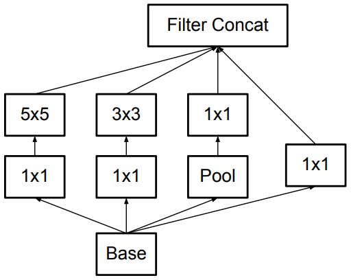
J. Imaging 2019, 5, 37                                                                              2 of 11

network (CNN). Arevalo et al. [6] tested various CNNs and compared them with two hand-crafted
descriptors for the task of mass diagnosis. Their experimentation was conducted on the BCDR-FM
dataset. They reported performance improvement with the combination of both learned and
hand-crafted representations. However, the authors did not test the performance of pretrained
networks and used simpler CNN architectures. Carneiro et al. [7] used a pre-trained CNN that
was fine-tuned using unregistered mammograms and segmented microcalcification and masses.
They estimated the risk of developing breast cancer according to BIRADS. They concluded that the
pre-trained models are superior to the randomly initialised ones. Huynh et al. [8] used the AlexNet [9]
pre-trained without further fine-tuning it for the problem of mass diagnosis. They analyzed the
performance of classification using features from various intermediate layers of the network using
SVM for the classification. They compared their results to two approaches: a classifier operating on
hand-crafted features and an ensemble of both, using soft voting. Jiao et al. [10] proposed a scheme in
which a pre-trained CNN was fine-tuned on a subset of DDSM database. Then, features of masses
were extracted from different layers of this model. In this way ‘high-level’ and ‘middle-level’ features
were obtained that correspond to different scales. Two linear SVM classifiers are trained for the
decision procedure, one for each feature group, and their predictions are fused. Levy and Jain [11]
classified mammographic masses using AlexNet and GoogleNet. They compared transfer learning to
from-scratch training finding that the former achieves superior results. It is worth noting that they
investigated the effect of data context, concluding that cropping larger bounding boxes of fixed size
around the lesion is more effective compared to cropping with proportional padding. Ting et al. [12]
created and trained from scratch their network for breast mass classification. Their network comprises
28 convolutional and fully-connected layers and it is fed by proposal ROIs detected by an one-shot
detector. They conducted their experiments in MIAS database. Rampun et al. [13] used an ensemble of
a slightly modified version of AlexNet pre-trained and fine-tuned on CBIS-DDSM. During inference,
they picked the three best performing models and fused their predictions.
      The majority of state-of-the-art works proposes the utilization of pre-trained networks against
training from scratch. However, state-of-the-art networks are designed and tested on much more
diverse datasets, different in nature and several orders of magnitude larger than the available
mammographic datasets. Consequently, the capacity and complexity of such networks may by
far exceed the needs of smaller datasets, leading to major adverse effects when training from scratch.
As a result, several works have appeared whose authors propose from-scratch training.
      Considering the above, in this paper we investigate the performance of multiple networks.
We compare the performance of each network in two scenarios: the first scenario involves initiating
the training with pre-trained weights while for the second the networks are initialized with
random weights.
      The remainder of the paper is organized as follows: Section 2 details the deep learning
architectures used in the current study for the classification of mammograms as benign or malignant.
Section 3 presents the experimental setup along with the corresponding results. Finally, in Section 4
conclusions are drawn.

2. Methodology

2.1. Convolutional Neural Networks

2.1.1. AlexNet
     AlexNet [9] was the first convolutional neural network (CNN) that exhibited performance beyond
the state-of-the-art in the task of object detection and classification. As shown in Figure 1, the network
contains eight layers; the first five are convolutional an the remaining three are fully-connected.
The first layer of the network filters the input image (sized 224 × 224) with 96 kernels of size 11 × 11
with a stride of 4 pixels. The depth of these kernels equals the number of channels of the input image.
The second layer takes as input the output of the first layer, after local response normalization and
J. Imaging 2019, 5, 37 3 of 11
max-pooling have been applied, filtering it with 256 kernels of size 5 × 5 × 96. The third, fourth
and fifth layers are connected to one another without any intervening pooling or normalization
layers. The third layer has 384 kernels of size 3 × 3 × 256. The fourth layer has 384 kernels of size
3 × 3 × 384 and the fifth layer has 256 kernels of size 3 × 3 × 384. On top of the convolutional layers,
two fully-connected layers are connected that have 4096 neurons each. The number of neurons in the
third fully-connected layer equals the number of classes.
Along with the particular architecture of the network, the authors of [9] also introduced some
novel features that greatly contribute to the network’s ability to learn and generalize. The most
important feature is that they replaced the standard neuron activation functions (logistic function and
hyperbolic tangent) with the rectified linear function f ( x ) = max(0, x ). Neurons that use this activation
function are referred to as Rectified Linear Units (ReLUs). The advantage of this activation function is
that it imposes a non-saturating non-linearity in contrast to sigmoid functions that saturate for large
values. This allows for significantly better flow of the gradients along with improved calculations
efficiency. ReLUs are established as the standard choice of activation function for CNNs. The authors
also introduced a depth-wise normalization scheme for each location of the feature maps produced by
a convolutional layer, called Local Response Normalization (LRN). This sort of response normalization
creates a competition for big activities amongst neuron outputs computed using different kernels.
While LRN was adopted and incorporated into various other network architectures, it was removed
from AlexNet in a subsequent publication [14].
A particularly important aspect of training was the use of dropout [15] (with probability of 0.5) for
the three fully-connected layers. This technique consists of setting to zero the output of each hidden
neuron with some probability. The neurons that are picked contribute to neither the forward pass nor
the back-propagation. Thus, in every training iteration, a different architecture is sampled. The dropout
technique acts as a regularizer, forcing the network to learn meaningful features, but increases the
training time.
Convolutional
Fully Connected Layers,
Input 96 kernels, 11x11
4096 neurons
stride 4
Convolutional
96 kernels
5x5
Convolutional Convolutional Convolutional
384 kernels 384 kernels 256 kernel
3x3 3x3 3x3 Softmax Layer
14x14x256
14x14x384
14x14x384
224x224x3
28x28x96
28x28x96
14x14x96
56x56x96
7x7x256
Output
Max Pooling, 2x2
Max Pooling, 2x2
Max Pooling, 2x2
Figure 1. AlexNet structure.J. Imaging 2019, 5, 37 4 of 11
2.1.2. VGG
In [16] authors investigated the effect of network depth while keeping the convolution filters
very small. They showed that significant improvement can be achieved by pushing the depth to
16–19 layers. The input to the convolutional layer is a fixed-size 224 × 224 image. The image is passed
through a stack of convolutional layers with ReLU activations where filters with very small receptive
fields (3 × 3) were used. The convolution stride is also fixed to 1. Spatial pooling is carried out by five
max-pooling layers, performed after some of the convolutional layers. Similarly to AlexNet, a stack of
three fully-connected layers is put on top of the convolutional part of the network. The advantage of
VGG is that, by stacking multiple convolutional layers with small-sized kernels, the effective receptive
field of the network is increased, while reducing the number of parameters compared to using less
convolutional layers with larger kernels for the same receptive field.
The authors tested multiple configurations of varying depth (9, 11, 16, and 19 layers). In one of
the configurations 1 × 1 filters were utilized, which can be seen as a linear transformation of the input
channels. This is also a way to increase the non-linearity of the decision function without affecting
the receptive fields of the convolutional layers. One of the configurations also included a LRN layer.
As reported in the paper, best results were achieved for depths between 16 and 19. The architecture of
VGG-16 is depicted in Figure 2.
Conv1: 2 Layers Fully Connected Layers,
Input
64 kernels, 3x3 4096 neurons
Conv2: 2 Layers
128 kernels, 3x3
Conv3: 3 Layers
256 kernels, 3x3
Conv4: 3 Layers
512 kernels, 3x3 Softmax Layer
Conv5: 3 Layers
512 kernels, 3x3
112x112x128
112x112x128
224x224x64
224x224x64
112x112x64
14x14x512
224x224x3
56x56x128
56x56x256
56x56x256
56x56x256
28x28x256
28x28x512
28x28x512
28x28x512
14x14x512
14x14x512
14x14x512
7x7x512
Output
Max Pooling, 2x2
Max Pooling, 2x2
Max Pooling, 2x2
Max Pooling, 2x2
Max Pooling, 2x2
Figure 2. VGG-16 structure.
2.1.3. GoogLeNet/Inception
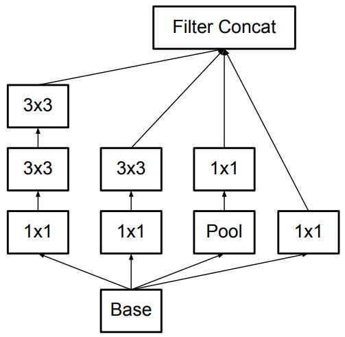
GoogLeNet [17] is the first implementation using the Inception module. The main idea behind this
module is based on authors’ findings about how a local sparse structure can be approximated by dense
components. Their aim was to find the optimal local structure and repeat it, constructing a multi-layer
network. The Inception module comprises four branches that get the same input (Figure 3a). The first
branch filters the input with a 1 × 1 convolution, which acts as a linear transformation on input
channels. The second and third branches perform 1 × 1 kerneled convolutions for dimensionality
reduction followed by convolutional layers with kernels of size 3 × 3 and 5 × 5, respectively. The fourth
branch performs max-pooling followed by convolution with 1 × 1 kernels. Finally, the outputs of eachJ. Imaging 2019, 5, 37 5 of 11
branch are concatenated and fed as input to the next block. GoogLeNet is constructed by stacking nine
Inception modules. In selected locations a max-pooling layer is placed between inception modules
in order to decrease the dimensionality of the feature maps. A feature of GoogLeNet worth noting
is the incorporation of auxiliary classifiers. Based on the assumption that middle layers of a CNN
should produce discriminative features, the authors added simple classifiers (two fully connected
and a softmax layer) that operate on the features produced by an intermediate point of the network.
The loss calculated by the decisions of these classifiers is used during the back-propagation stage to
calculate additional gradients that contribute to the training of the respective convolutional layers.
At inference time the auxiliary classifiers are discarded.
(a) (b)
Figure 3. (a) Inception module of GoogLeNet; (b) Inception-v2 module.
In subsequent publications [18], a revised version of the Inception module have been proposed,
along with slightly modified network architectures. The authors proposed Batch Normalization (BN)
and incorporated it into the Inception network. BN is a technique that makes normalization part of the
model architecture, performing the normalization for each training mini-batch. The authors argue that
BN allows for higher learning rates and simpler initialization techniques without experiencing adverse
effects. According to BN, all the images of the current mini-batch are rescaled so that they have mean
value of 0 and variance of 1. Consequently, a linear transform is applied, the parameters of which
are learned through the training process. The network that was used in [18], namely Inception-v2,
was a slight modification of GoogLeNet. Apart from the incorporation of BN, the most important
change is that the 5 × 5 convolutional layers of the Inception module were replaced by two consecutive
3 × 3 layers (Figure 3b).
2.1.4. Residual Networks
Residual networks (ResNets) [19] consist of reformulated convolutional layers that are learning
residual functions with reference to the inputs. The authors argue that this type of networks are easier
to optimize and can be of significantly increased depth. The implementation of a “residual block”,
as described in [19], is straightforward: for every few convolutional layers a “shortcut connection”
is added that runs parallel to these layers and implements the identity mapping. The output of the
convolutional layers is then added to the output of the shortcut branch and the result is propagated
to the subsequent block (Figure 4). Beside the use of shortcut connections, the network architecture
is mainly inspired by the philosophy of VGG networks. All convolutional layers have small kernels
of size 3 × 3 and follow two simple design rules: (i) for the same output feature map size, the layers
have the same number of filters; (ii) when the feature map size is halved (with convolutional layers of
stride 2), the number of filters is doubled so as to preserve the time complexity per layer. The authors
tested architectures of varying depth in the range between 34 and 152 layers.J. Imaging 2019, 5, 37 6 of 11
Figure 4. Building block of ResNet [19].
3. Experimental Results
In this work we aim to explore the performance of deep convolutional neural networks, in the
context of breast mass classification into benign or malignant, in the case of (a) training from scratch
and (b) fine-tuning. For the performance evaluation two datasets were used:
DDSM-400
This dataset consists of 400 mass ROIs extracted from the Digital Database for Screening
Mammography (DDSM) [20] that was developed and used in our previous work [21]. The selected
dataset was enriched due to a further processing of the ROIs, performed by expert radiologists, in order
to acquire an accurate mass contour delineation using a semi-automatic segmentation method [22].
Two benign and two malignant samples from the dataset are depicted in Figure 5a.
CBIS-DDSM
The Curated Breast Imaging Subset of DDSM (CBIS-DDSM) [23] is an updated and standardized
version of DDSM. It contains 10,239 mammographic images, linked to normal, benign, and malignant
cases, selected and curated by a trained mammographer. The images are converted to the DICOM
format and an updated ROI segmentation is provided for each lesion. The dataset is split to training
and testing subsets to facilitate the direct comparison of performance between different methodologies.
For this study, only cases concerning masses where extracted totaling 1319 and 378 ROIs for training
and testing, respectively. Two benign and two malignant samples from the dataset are depicted in
Figure 5b.
(a)
(b)
Figure 5. Two benign and two malignant samples from (a) the Curated Breast Imaging Subset of DDSM
(CBIS-DDSM) and (b) DDSM-400.J. Imaging 2019, 5, 37 7 of 11
For the experiments concerning training networks from scratch the Glorot initialization [24]
method was used. For the fine-tuning experiments the networks were initialized with the pre-trained
weights from the ImageNet dataset [25]. The fully connected layers of the pre-trained networks
were removed and replaced with randomly initialized ones. The final layer of each network is fully
connected, containing two softmax neurons for the binary classification problem at hand. For the
training process the Adam optimization method [26] was employed. Multiple learning rates were
tested for each network at each scenario, which varied between 10−4 and 10−7 . The batch size varied
from 10 to 32 images, constrained by the memory requirements of each configuration. Early stopping
was also used, terminating the training process if the AUC on the validation set did not improve for
15 consecutive epochs. The input image size was set to 224 × 224. Table 1 summarizes the training
parameters used for each network.
Table 1. Network parameters in the case of fine-tuning (FT) and from-scratch (SC) training scenarios.
Learning Rate Best Model Iter.
CNN Number of Weights Batch Size
FT SC FT SC
AlexNet 56, 866, 848 32 10−5 10−5 6 65
VGG-16 134, 256, 320 32 10−5 10−5 9 58
VGG-19 139, 564, 736 32 10−5 10−5 14 64
ResNet-50 23, 512, 128 32 10−5 10−4 4 104
ResNet-101 42, 504, 256 16 10−5 10−5 13 92
ResNet-152 58, 147, 904 10 10−5 10−7 31 38
GoogLeNet 10, 299, 840 32 10−5 10−5 12 12
Inception-BN (v2) 16, 072, 832 32 10−4 10−5 43 108
The evaluation process for the DDSM-400 dataset is conducted employing 10-fold cross validation.
Specifically, the dataset is partitioned randomly into 10 non-overlapping subsets of 40 samples. For each
folding, the remaining 360 samples are further split to training (80%) and validation (20%) sets in
a random fashion. The results provided for this dataset are calculated as the average of the ten runs.
For the CBIS-DDSM dataset we used the original training partitioning which, similarly to DDSM-400,
was randomly split to a new training set and a validation set.
The extraction of ROIs from the mammograms was performed by cropping a window of fixed
size (1024 × 1024) for all lesions, centered around the mass. The image size was selected as such in
order to be sufficient for all the masses in the dataset. In this way, resize-induced distortion is avoided
while sufficient adjacent tissue is included for learning features in larger scales.
Data augmentation is an important part of the training process of deep networks. Through
data augmentation, artificial training samples are generated by transforming existing images.
The transformations used in our experimentation are rotation and flipping. In this way, meaningful
samples are generated implying rotation invariance for the learned features. The data augmentation
process is performed online, i.e., for each training sample random rotation and flipping is applied.
Tables 2 and 3 summarize the performance of multiple networks, for the fine-tuning and
from-scratch training scenarios, respectively. The metrics used for the performance evaluation are the
area under ROC curve (AUC) and the classification accuracy (ACC).
As shown in Tables 2 and 3 and Figure 6, CNNs trained under the fine-tuning scenario achieved
better performance compared with the ones trained from scratch. This confirms the tendency in
state-of-the-art works to show a preference to the fine-tuning scenario. This difference in performance is
attributed to the fact that the examined networks are designed and optimized for datasets several orders
of magnitude larger than the available mammographic ones. However, once the network is trained,
the learned features can address a variety of problems different in nature, after a fine-tuning stage.J. Imaging 2019, 5, 37 8 of 11
Table 2. Performance of deep neural networks using the from-scratch training scenario.
DDSM-400 CBIS-DDSM
CNN
AUC ACC AUC ACC
AlexNet 0.657 0.610 0.716 0.656
VGG-16 0.621 0.590 0.702 0.580
VGG-19 0.644 0.588 0.707 0.581
ResNet-50 0.595 0.548 0.637 0.627
ResNet-101 0.637 0.588 0.641 0.662
ResNet-152 0.596 0.543 0.609 0.647
GoogLeNet 0.580 0.569 0.590 0.598
Inception-BN (v2) 0.652 0.590 0.577 0.654
Table 3. Performance of convolutional neural networks (CNNs) initialized on pre-trained weights
(fine-tuning).
DDSM-400 CBIS-DDSM
CNN
AUC ACC AUC ACC
AlexNet 0.805 0.733 0.802 0.753
VGG-16 0.844 0.748 0.781 0.716
VGG-19 0.835 0.738 0.783 0.736
ResNet-50 0.856 0.743 0.804 0.749
ResNet-101 0.859 0.785 0.791 0.753
ResNet-152 0.786 0.630 0.793 0.755
GoogLeNet 0.830 0.758 0.767 0.720
Inception-BN (v2) 0.850 0.780 0.774 0.747
Maximum performance was achieved using fine-tuning in ResNet-50 and ResNet-101 in both
datasets. This coincides with the results reported in ILSVCR competition [27] as well. A counter-intuitive
outcome of our investigation is that ResNets achieve low performance in the from-scratch training
scenario, compared to AlexNet and VGG, which are of much higher capacity (Table 1), which is known
to lead in over-fitting for small datasets. A possible cause for this is the increased complexity of ResNet,
as it is an order of magnitude deeper than the other networks studied in our paper. As convolutional
neural networks become deeper, i.e., with larger number of layers, the number of non-linearities is
also increased, which results in more difficult convergence and increases the possibility of over-fitting.
In the case of from-scratch training, maximum performance was achieved with AlexNet, which is the
simpler and shallower network tested. This confirms the hypothesis that, when it comes to datasets
with limited numbers of samples, such as the ones available for medical applications and specifically
mammography, effective training of larger and complex networks cannot be achieved.
Table 4 shows the performance reported in three state-of-the-art methods, which exploit
hand-crafted features for breast cancer diagnosis. The top-performing networks achieve marginally
increased performance from [21] and surpass all the other works, when evaluated on the same dataset,
in terms of AUC. However, the architecture developed in [21] utilizes a detailed lesion segmentation,
provided as input, to extract shape features. Consequently, the performance of the system is highly
dependent on the quality of the provided segmentation, that can be a task that requires significant
time and effort spent from the user. In contrast, the lack of any dependencies in CNN results in a more
concrete end-to-end classification system where diagnosis can be fully automated.J. Imaging 2019, 5, 37 9 of 11
0.9
0.8
AUC
From-Scratch
0.7
Fine-tuning
0.6
0.5
t 6 9 0 1 2 et v2
xNe VGG-1 VGG-1 sNet-5 Net-10 Net-15 ogLeN ption-
Ale e s s Go e
R Re Re Inc
(a) DDSM-400
0.9
0.8
AUC
From-Scratch
0.7
Fine-tuning
0.6
0.5
t 6 9 0 1 2 et v2
xNe VGG-1 VGG-1 sNet-5 Net-10 Net-15 ogLeN ption-
Ale Re Res Res Go Ince
(b) CBIS-DDSM
Figure 6. Performance of convolutional neural networks for from-scratch and fine-tuning scenarios in
terms of AUC for (a) DDSM-400 and (b) CBIS-DDSM.
Table 4. Performance of state-of-the-art methods based on hand-crafted features.
DDSM-400
Method
AUC ACC
Tsochatzidis et al. [21] 0.85 0.81
Rouhi et al. [28] 0.78 0.79
Xie et al. [29] 0.72 0.68
4. Discussion and Concluding Remarks
In this paper, the use of deep convolutional neural networks for breast cancer diagnosis from
mammograms with mass lesions is investigated. The performance of various networks is assessed
on two digitized mammogram databases of different sizes. The first database comprises 400 images
from DDSM while the other comprises 1696. Two scenarios of training are considered: from-scratch,
where the weights of the network are initialized from random distributions, and fine-tuning, where
the training is initialized by weights of a network that has already been trained using another dataset.
From-scratch training is a tedious process as it requires the convergence of all the network
parameters, starting from a random state. On the one hand, increasing the depth of networks leadsJ. Imaging 2019, 5, 37 10 of 11
to better features in terms of discriminating ability; on the other hand, increasing depth makes the
network prone to various adverse effects, such as vanishing or exploding gradients and overfitting.
Although several improvements of the training process and network architecture have been proposed
to eliminate the complications imposed by the growing capacity and complexity of the models,
a major requirement for an effective training is still a large amount of data, which is not available
for most medically oriented applications, such as the problem at hand, i.e., breast cancer diagnosis
in mammograms.
In contrast, a fine-tuning training scenario for a CNN is naturally a simpler process, and puts
emphasis on domain-specific features rather than generic low-level ones. In this way it applies major
corrections of network parameters only for layers that are closer to the end of the network, where
higher-level concepts are captured.
Having that in mind, we would like to emphasize the need for assembling and constructing
large-scale mammographic datasets to support the active research fields of computer-aided detection
and diagnosis, specifically aimed for more advanced imaging modalities such as digital mammography,
which is the current standard and tomosynthesis that has an emerging role for imaging specific patient
groups [30].
Author Contributions: Conceptualization, L.T., L.C. and I.P.; Methodology, L.T.; Software, L.T.; Supervision, L.C.
and I.P.; Writing—original draft, L.T.; Writing—review & editing, L.C. and I.P.
Funding: This research received no external funding.
Acknowledgments: We gratefully acknowledge the support of NVIDIA Corporation with the donation of the
Titan Xp GPU used for this research.
Conflicts of Interest: The authors declare no conflict of interest.
References
1. Siegel, R.L.; Miller, K.D.; Jemal, A. Cancer statistics, 2015. CA Cancer J. Clin. 2015, 65, 5–29. [CrossRef]
[PubMed]
2. American Cancer Society. Breast Cancer Facts & Figures; American Cancer Society, Inc.: Atlanta, GA,
USA, 2015.
3. Eurostat. Health Statistics: Atlas on Mortality in the European Union; Office for Official Publications of the
European Union: Luxembourg, 2009.
4. Hubbard, R.A.; Kerlikowske, K.; Flowers, C.I.; Yankaskas, B.C.; Zhu, W.; Miglioretti, D.L. Cumulative
probability of false-positive recall or biopsy recommendation after 10 years of screening mammography:
A cohort study. Ann. Intern. Med. 2011, 155, 481–492. [CrossRef] [PubMed]
5. Hamidinekoo, A.; Denton, E.; Rampun, A.; Honnor, K.; Zwiggelaar, R. Deep learning in mammography and
breast histology, an overview and future trends. Med. Image Anal. 2018, 47, 45–67. [CrossRef] [PubMed]
6. Arevalo, J.; González, F.A.; Ramos-Pollán, R.; Oliveira, J.L.; Lopez, M.A.G. Representation learning
for mammography mass lesion classification with convolutional neural networks. Comput. Methods
Programs Biomed. 2016, 127, 248–257. [CrossRef] [PubMed]
7. Carneiro, G.; Nascimento, J.; Bradley, A.P. Unregistered multiview mammogram analysis with pre-trained
deep learning models. In Proceedings of the International Conference on Medical Image Computing
and Computer-Assisted Intervention, Munich, Germany, 5–9 October 2015; Springer: Berlin/Heidelberg,
Germany, 2015; pp. 652–660.
8. Huynh, B.Q.; Li, H.; Giger, M.L. Digital mammographic tumor classification using transfer learning from
deep convolutional neural networks. J. Med. Imaging 2016, 3, 034501. [CrossRef] [PubMed]
9. Krizhevsky, A.; Sutskever, I.; Hinton, G.E. Imagenet classification with deep convolutional neural
networks. In Proceedings of the Advances in Neural Information Processing Systems, Lake Tahoe, NV, USA,
3–6 December 2012; pp. 1097–1105.
10. Jiao, Z.; Gao, X.; Wang, Y.; Li, J. A deep feature based framework for breast masses classification.
Neurocomputing 2016, 197, 221–231. [CrossRef]J. Imaging 2019, 5, 37 11 of 11
11. Lévy, D.; Jain, A. Breast mass classification from mammograms using deep convolutional neural networks.
arXiv 2016, arXiv:1612.00542.
12. Ting, F.F.; Tan, Y.J.; Sim, K.S. Convolutional neural network improvement for breast cancer classification.
Expert Syst. Appl. 2019, 120, 103–115. [CrossRef]
13. Rampun, A.; Scotney, B.W.; Morrow, P.J.; Wang, H. Breast Mass Classification in Mammograms using
Ensemble Convolutional Neural Networks. In Proceedings of the 20th International Conference on e-Health
Networking, Applications and Services (Healthcom), Ostrava, Czech Republic, 17–20 September 2018; IEEE:
Piscataway, NJ, USA, 2018; pp. 1–6.
14. Krizhevsky, A. One weird trick for parallelizing convolutional neural networks. arXiv 2014, arXiv:1404.5997.
15. Hinton, G.E.; Srivastava, N.; Krizhevsky, A.; Sutskever, I.; Salakhutdinov, R.R. Improving neural networks
by preventing co-adaptation of feature detectors. arXiv 2012, arXiv:1207.0580.
16. Simonyan, K.; Zisserman, A. Very deep convolutional networks for large-scale image recognition. arXiv
2014, arXiv:1409.1556.
17. Szegedy, C.; Liu, W.; Jia, Y.; Sermanet, P.; Reed, S.; Anguelov, D.; Erhan, D.; Vanhoucke, V.; Rabinovich, A.
Going deeper with convolutions. In Proceedings of the IEEE Conference on Computer Vision and Pattern
Recognition, Boston, MA, USA, 7–12 June 2015; pp. 1–9.
18. Ioffe, S.; Szegedy, C. Batch normalization: Accelerating deep network training by reducing internal covariate
shift. In Proceedings of the International Conference on Machine Learning, Lille, France, 6–11 July 2015;
pp. 448–456.
19. He, K.; Zhang, X.; Ren, S.; Sun, J. Deep residual learning for image recognition. In Proceedings of the IEEE
Conference on Computer Vision and Pattern Recognition, Las Vegas, NV, USA, 27–30 June 2016; pp. 770–778.
20. Heath, M.; Bowyer, K.; Kopans, D.; Kegelmeyer, P., Jr.; Moore, R.; Chang, K.; Munishkumaran, S.
Current status of the digital database for screening mammography. In Digital Mammography; Springer:
Berlin/Heidelberg, Germany, 1998; pp. 457–460.
21. Tsochatzidis, L.; Zagoris, K.; Arikidis, N.; Karahaliou, A.; Costaridou, L.; Pratikakis, I. Computer-aided
diagnosis of mammographic masses based on a supervised content-based image retrieval approach.
Pattern Recognit. 2017, 71, 106–117. [CrossRef]
22. Arikidis, N.; Vassiou, K.; Kazantzi, A.; Skiadopoulos, S.; Karahaliou, A.; Costaridoua, L. A two-stage method
for microcalcification cluster segmentation in mammography by deformable models. Med. Phys. 2015,
42, 5848–5861.
23. Lee, R.S.; Gimenez, F.; Hoogi, A.; Miyake, K.K.; Gorovoy, M.; Rubin, D. A curated mammography data set
for use in computer-aided detection and diagnosis research. Sci. Data 2017, 4, 170–177.
24. Glorot, X.; Bengio, Y. Understanding the difficulty of training deep feedforward neural networks.
In Proceedings of the Thirteenth International Conference on Artificial Intelligence and Statistics, Chia
Laguna Resort, Sardinia, Italy, 13–15 May 2010; pp. 249–256.
25. Deng, J.; Dong, W.; Socher, R.; Li, L.J.; Li, K.; Fei-Fei, L. Imagenet: A large-scale hierarchical image database.
In Proceedings of the 2009 IEEE Conference on Computer Vision and Pattern Recognition (CVPR 2009),
Miami, FL, USA, 20–25 June 2009; IEEE: Piscataway, NJ, USA, 2009; pp. 248–255.
26. Kingma, D.P.; Ba, J. Adam: A method for stochastic optimization. arXiv 2014, arXiv:1412.6980.
27. Russakovsky, O.; Deng, J.; Su, H.; Krause, J.; Satheesh, S.; Ma, S.; Huang, Z.; Karpathy, A.; Khosla, A.;
Bernstein, M.; et al. ImageNet Large Scale Visual Recognition Challenge. Int. J. Comput. Vis. 2015,
115, 211–252. [CrossRef]
28. Rouhi, R.; Jafari, M.; Kasaei, S.; Keshavarzian, P. Benign and malignant breast tumors classification based on
region growing and CNN segmentation. Expert Syst. Appl. 2015, 42, 990–1002. [CrossRef]
29. Xie, W.; Li, Y.; Ma, Y. Breast mass classification in digital mammography based on extreme learning machine.
Neurocomputing 2016, 173, 930–941. [CrossRef]
30. Oeffinger, K.C.; Fontham, E.T.; Etzioni, R.; Herzig, A.; Michaelson, J.S.; Shih, Y.C.T.; Walter, L.C.; Church, T.R.;
Flowers, C.R.; LaMonte, S.J.; et al. Breast cancer screening for women at average risk: 2015 guideline update
from the American Cancer Society. JAMA 2015, 314, 1599–1614. [CrossRef] [PubMed]
c 2019 by the authors. Licensee MDPI, Basel, Switzerland. This article is an open access
article distributed under the terms and conditions of the Creative Commons Attribution
(CC BY) license (http://creativecommons.org/licenses/by/4.0/).You can also read