Attribute Selection Based on Constraint Gain and Depth Optimal for a Decision Tree - MDPI
←
→
Page content transcription
If your browser does not render page correctly, please read the page content below
entropy
Article
Attribute Selection Based on Constraint Gain and
Depth Optimal for a Decision Tree
Huaining Sun 1, * , Xuegang Hu 2 and Yuhong Zhang 2
 1   School of Computer Science, Huainan Normal University, Huainan 232038, China
 2   School of Computer and Information, Hefei University and Technology, Hefei 230009, China;
     jsjxhuxg@hfut.edu.cn (X.H.); zhangyuhong99@163.com (Y.Z.)
 *   Correspondence: sunhncn@126.com; Tel.: +86-0554-6887433

 Received: 2 January 2019; Accepted: 13 February 2019; Published: 19 February 2019

 Abstract: Uncertainty evaluation based on statistical probabilistic information entropy is a commonly
 used mechanism for a heuristic method construction of decision tree learning. The entropy kernel
 potentially links its deviation and decision tree classification performance. This paper presents
 a decision tree learning algorithm based on constrained gain and depth induction optimization.
 Firstly, the calculation and analysis of single- and multi-value event uncertainty distributions of
 information entropy is followed by an enhanced property of single-value event entropy kernel and
 multi-value event entropy peaks as well as a reciprocal relationship between peak location and the
 number of possible events. Secondly, this study proposed an estimated method for information
 entropy whose entropy kernel is replaced with a peak-shift sine function to establish a decision tree
 learning (CGDT) algorithm on the basis of constraint gain. Finally, by combining branch convergence
 and fan-out indices under an inductive depth of a decision tree, we built a constraint gained and
 depth inductive improved decision tree (CGDIDT) learning algorithm. Results show the benefits of
 the CGDT and CGDIDT algorithms.

 Keywords: decision tree; attribute selection measure; entropy; constraint entropy; constraint gain;
 branch convergence and fan-out

1. Introduction
      Decision trees are used extensively in data modelling of a system and rapid real-time prediction
for real complex environments [1–5]. Given a dataset acquired by field sampling, a decision attribute is
determined through a heuristic method [6,7] for training a decision tree. Considering that the heuristic
method is the core of induction to a decision tree, many researchers have contributed substantially to
studying an inductive attribute evaluation [8–10]. Currently, the heuristic method of attribute selection
remains an interesting topic in improving learning deviation.
      The attribute selections in constructing a decision tree are mostly based on the uncertainty heuristic
method, which can be divided into the following categories: Information entropy method based on
statistical probability [11–14], based on a rough set and its information entropy method [15–17],
and the uncertainty approximate calculation method [18,19]. An uncertainty evaluation of Shannon
information entropy [20] based on statistical probability has been used previously for uncertainty
evaluation of the sample set division of decision tree training [21], such as the well-known ID3 and
C4.5 heuristic method of the decision tree algorithm [22,23]; these methods are used to search for
a gain-optimized splitting feature of dividing subsets for an inductive classification to achieve a
rapid convergence effect. Whilst a rough set has the advantage of natural inaccuracy expression,
through the dependency evaluation of condition and decision attributes, the kernel characteristics
of its strong condition quality is selected as the split attribute to form the decision tree algorithm,

Entropy 2019, 21, 198; doi:10.3390/e21020198                                  www.mdpi.com/journal/entropy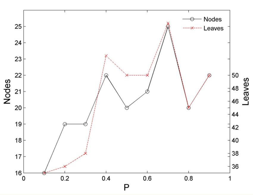
Entropy 2019, 21, 198                                                                                    2 of 17

with improved classification performance [15–17,24]. The uncertainty approximation calculations
focus on the existence of the deviation in an evaluation function estimated by most learning methods
with information theory [18]. These computations further improve the stability of the algorithm by
improving the uncertainty estimation of entropy [25–28]. The deviation in entropy is not only from
itself, but also from the properties of data and samples.
      This study proposed an improved learning algorithm based on constraint gain and depth induction
for a decision tree. To suppress the deviation of entropy itself, we firstly used a peak-shift sine factor that
is embedded in the information entropy to create a constraint gain GCE heuristic in accordance with the
entropy law of peak, which moves to a low probability and intensity enhancement whilst increasing the
number of events possible. The uncertainty is represented moderately so that the estimation deviation
could be avoided. This phenomenon realizes the uncertainty estimation considering the otherness of
the data property while allowing for entropy itself. Moreover, evaluation indicators of branch inductive
convergence and fan-out are used in assisting the heuristic GCE to select a minimal attribute that is affected
by data samples and noises on the basis of the primary attributes. This study obtained an improved
learning algorithm through an uncertainty-optimized estimation for the attributes of a decision tree.
The experimental results validate the effectiveness of our proposed method.
      The rest of this paper is organized as follows. Section 2 introduces some related works on the attribute
selection of heuristic measures in a decision tree. Section 3 discusses the evaluation of uncertainty. Section 4
proposes a learning algorithm based on the constraint gain and optimal depth for a decision tree. Section 5
introduces the experimental setup and results. Section 6 concludes the paper.

2. Related Work
     Decision tree learning aims to reduce the distribution uncertainty of a dataset, which is partitioned
by selected split attributes, and enables a classified model of induction to be simple and reasonable.
Notably, a heuristic model based on the uncertainty of entropy evaluation has become a common
pattern for decision tree learning given its improved uncertainty interpretation.
     The uncertainty evaluation based on information entropy was design by Quinlan in the
ID3 algorithm [22] in which the uncertainty entropy of a class distribution, H(C), is reduced by
the class distribution uncertainty, E(A), of the attribute domain in the dataset, namely H(C)-E(A);
thus, a heuristic method of information gain with an intuitive interpretation is obtained. Given that
H(C) is a constant of the corresponding dataset, the information gain is the minimum calculation
of the Gain uncertainty at the core, E(A). In the attribute domain of E(A), a small distribution of the
classification uncertainty is easily obtained using multi-valued attributes, thereby leading to an evident
multi-valued attribute selection bias and splitting of the attribute selection instability in the Gain
heuristic. The C4.5 algorithm [23] uses an H(A) entropy to normalise Gain in an attempt to suppress the
bias of a split attribute selection; furthermore, this algorithm improves the classification performance
of a decision tree through a pruning operation. Some authors [14] used a class constraint entropy to
calculate the uncertainty of the attribute convergence and achieved an improved attribute selection
bias and performance.
     Nowozin [18] considered information entropy to be biased and proposed the use of discrete
and differential entropy to replace the uncertainty estimation operator of a traditional information
entropy. These authors found that improving the predictive performance originates from enhancing
the information gain.
     Wang et al. [29] introduced the embedding of interest factors in the Gain heuristic, E(A),
in which the process is simplified as a division operation of a product, and the sum of the
category sample accounts for each attribute to form an improved PVF-ID3 algorithm. According to
Nurpratami et al. [30], space entropy denotes that the ratio of the class inner distance to the outer
distance is embedded in information entropy. Then, space entropy is utilised, rather than information
entropy, to constitute the information gain estimation between the target attribute and support
information to achieve hot and non-hot spot heuristic predictions.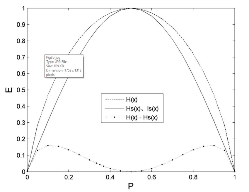
Entropy 2019, 21, 198 3 of 17
Sivakumar et al. [31] proposed to use Renyi entropy to replace the information entropy in the
Gain heuristic. Moreover, the normalisation factor, V(k), was used to improve the Gain instability,
thereby improving the performance of the decision tree. Wang et al. [29] suggested to replace the
entropy of information gain with unified Tsallis entropy and determined the optimal heuristic method
through q parameter selection. Some authors [32] proposed that the deviation of the Shannon entropy
is improved by the sine function-restraining entropy peak, but the impact of the property distribution
and data sampling imbalance should be ignored.
In addition, Qiu C et al. [33] introduced a randomly selected decision tree, which aims to keep the
high classification accuracy while also reducing the total test cost.
3. Measure of Uncertainty
3.1. Analysis of Uncertainty Measure of Entropy
The concept of entropy has been previously utilized to measure the degree of disorder in a
thermodynamic system. Shannon [20] introduced this thermodynamic entropy into information theory
to define the information entropy.
We assume that a random variable, Xj , who has v possible occurrence can be obtained from
things’ space. If we aimed to measure the heterogeneity of things’ status through Xj , then its measured
information entropy is described as follows:
v v
H (Xj ) = ∑ P(Xjk ) I (Xjk ) = ∑ − P(Xjk ) log2 P(Xjk ) (1)
k =1 k =1
where Xj ∈A is a random variable derived from an attribute of things, A is the attribute set, and Xjk is
an arbitrary value of this attribute. P(Xjk ) is the occurrence probability of the event represented by this
attribute value. I(Xjk ) is the self-information of Xjk , and H(Xj ) is a physical quantity that measures the
amount of information provided by the random variable, Xj .
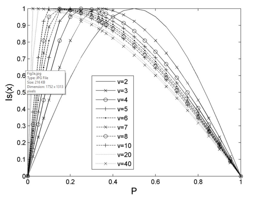
We assume that the number of possible values, v, is defined as 1 – 4 for a random variable, Xj .
Firstly, the occurrence probability of the event is generated by different parameter settings, and then
the distribution of the information entropy is calculated. The results of these calculations are illustrated
in Figures 1 and 2. The distribution of the information entropy of the single-value event is an
asymmetric convex peak, which changes steeply in a small probability region and slowly in a large
probability region. The position of the peak top is at P ≈ 0.36788, and the maximum value is Hmax (Xj )
= 0.53073, as depicted in Figure 1a. The distribution of the information entropy of a double-value
event is a symmetric convex peak with probability of P = 0.5 whose maximum value is Hmax (Xj ) = 1,
as demonstrated in Figure 1b. The distribution shape of the information entropy of a three-value
event. Three-value events are convex peaks with left steep and right slow, as exhibited in Figure 2a,b.
The preceding peak top is at P = 1/3, and its maximum value is Hmax (Xj ) ≈ 1.58496. The rear peak top
is at P = 0.25, and its maximum value is Hmax (Xj ) = 2.
When the number of values for a random variable is greater than 2, the peak of the information
entropy of the random variable not only moves regularly with the change in the values, but also
increases its peak intensity to greater than 1. Therefore, the deviation in the uncertainty estimation is
protruded by the change in the value number of the random variable, whereas the peak shift of the
information entropy presents the uncertainty distribution.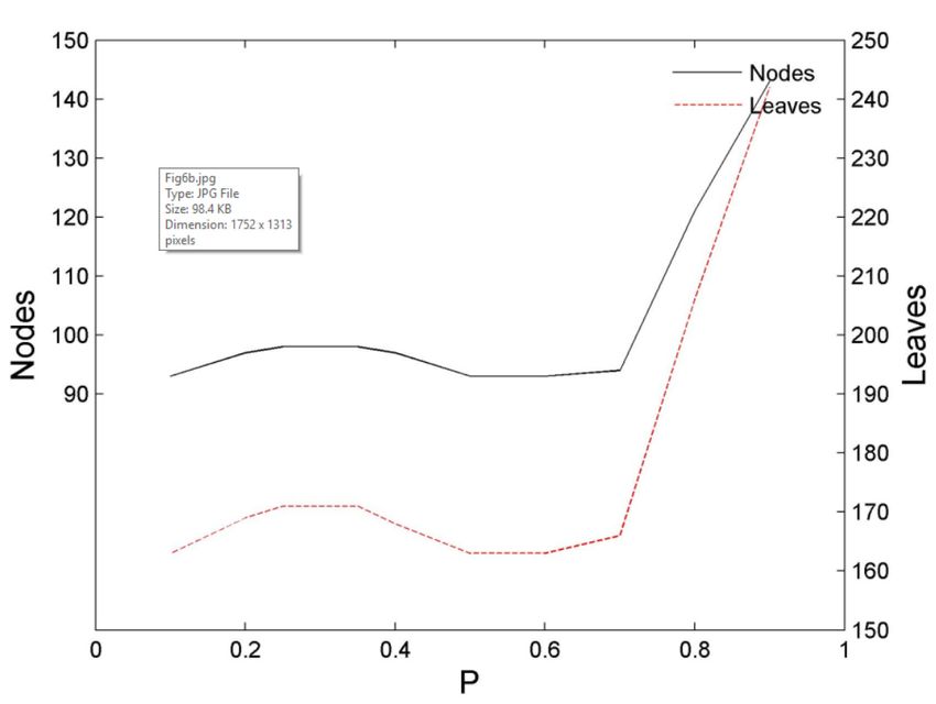
Entropy 2019,21,
Entropy2019, 21,198
x FOR PEER REVIEW 44 of
of 17
18
Entropy 2019, 21, x FOR PEER REVIEW 4 of 18
(a) (b)
(a) (b)
Figure 1. Entropy of single-value event and two-value event. (a) Comparison of I(x) and H(x) for a
Figure 1.1. Entropy
Figure Entropy of
of single-value
single-value event
event and
and two-value
two-value event.
event. (a) Comparison
Comparison of
of I(x)
I(x) and
and H(x)
H(x) for
for aa
single-value event; (b) Entropy, H(x), of two-value event.
single-value event;
single-value event; (b)
(b)Entropy,
Entropy,H(x),
H(x),of
oftwo-value
two-valueevent.
event.
(a) (b)
(a) (b)
Figure
Figure 2. Distribution analysis
2. Distribution analysisofofmulti-value
multi-valueevent evententropy.
entropy.(a)(a) Entropy
Entropy of of three-value
three-value event; event; (b)
Figure 2. Distribution analysis of multi-value event entropy. (a) Entropy of three-value event; (b)
(b) Entropy
Entropy of four-value
of four-value event.
event. Note:Note:
(1) If (1) If three
three possiblepossible probabilities
probabilities of theofeventthe event are P(X arej1),P(XP(Xj1j2),),
Entropy of four-value event. Note: (1) If three possible probabilities of the event are P(Xj1), P(Xj2),
P(X ), and
andj2P(X P(Xj3 ), respectively,
j3), respectively, let parameter k exist tok make
let parameter exist to
P(X j3) = kP(X
make k P(X
P(Xj3j2)), =then, P(X = [1 −P(X
j2 ),j2)then, = [1+−k)
P(Xj2j1))]/(1
and P(Xj3), respectively, let parameter k exist to make P(Xj3) = k P(Xj2), then, P(Xj2) = [1 − P(Xj1)]/(1 + k)
P(X j1 )]/(1 k+>k)0.in(2)
in which which
If fourk >possible
0. (2) If four possible of
probabilities probabilities
the event are of the
P(Xeventj1), P(X j2),P(X
are P(Xj1j3),), P(X ), P(X
andj2P(X ),
j4),j3let
in which k > 0. (2) If four possible probabilities of the event are P(Xj1), P(Xj2), P(Xj3), and P(Xj4), let
and P(Xj4 ), let
parameter k1and k2 exist kto
parameter 1 and
makek2 exist k1 P(XP(X
P(Xj3)to=make k1 P(X
j3 ) =P(X
j2) and P(Xj2P(X
j4) =j2k)2 and j4 ) = k
), then, 2 P(X
P(X = ),[1then,
j2) j2 − P (X P(X j2 ) =+
j1)]/(1
parameter k1and k2 exist to make P(Xj3) = k1 P(Xj2) and P(Xj4) = k2 P(Xj2), then, P(Xj2) = [1 − P (Xj1)]/(1 +
k1 −
[1 + kP2),(Xinj1 )]/(1
which + k1 >+ 0k2and
), in kwhich k1 > 0“1,1”
2 > 0. Sign and ksimilar
2 > 0. Sign “1,1” similar
to Figure (b), thetonumberFigure (b), the front
at the number is kat the
1, and
k1 + k2), in which k1 > 0 and k2 > 0. Sign “1,1” similar to Figure (b), the number at the front is k1, and
front is
the number k 1 , and the number
after it is k2. after it is k 2 .
the number after it is k2.
3.2. Definition of Constraint Entropy Estimation Based on Peak-Shift
When the number of values for a random variable is greater than 2, the peak of the information
When the number of values for a random variable is greater than 2, the peak of the information
entropyFor aofrandom
the random
variable, Xj ∈not
variable {X ,only moves
X2 ,..., Xm }, regularly with the the
which represents change in thetovalues,
attribute but that
the event also
entropy of the random variable not1only moves regularly with the change in the values, but also
increasesin
occurred itsthings’
peak intensity
space, ifto greater thanuncertainty
a reasonable 1. Therefore, the deviation
evaluation of thein X the uncertainty
variable on all estimation
attributes’
increases its peak intensity to greater than 1. Therefore, the deviation in jthe uncertainty estimation
is protruded
set is required, bythen
the change
the effect in of
thethevalue number
possible of theofrandom
number randomvariable,
variables whereas
on the the peak shift
intensity of
of the
is protruded by the change in the value number of the random variable, whereas the peak shift of
the information entropy presents the uncertainty distribution.
information entropy is eliminated. This condition aims to create a normalized measurement of
the information entropy presents the uncertainty distribution.
uncertainty. We define the entropy estimation to measure the uncertainty of this random variable
3.2. Definition of Constraint Entropy Estimation Based on Peak-Shift
as
3.2.follows:
Definition of Constraint Entropy Estimation Based v on Peak-Shift
For a random variable, Xj ∈{X1, Xj 2,..., k∑
For a random variable, Xj ∈{X H ( X ) = P ( X
sc 1, X2,..., Xm}, whichjk ) Isinrepresents
( X jk , v) the attribute to the event that (2)
X
=
m}, which represents the attribute to the event that
1
occurred in things’ space, if a reasonable uncertainty evaluation of the Xj variable on all attributes’
occurred in things’ space, if a reasonable uncertainty evaluation of the Xj variable on all attributes’
where Hsc is the then
set is required, average
the of the uncertainty
effect of the possible of anumber
randomof randomXvariables
variable, j . We aimon forthe
thisintensity
variable of
to the
be
set is required, then the effect of the possible number of random variables on the intensity of the
no more thanentropy
information 0.5 when is iteliminated.
is a single-value variable. aims
This condition The kernel,
to create Isin ,aofnormalized
the entropymeasurement
is the key part of
information entropy is eliminated. This condition aims to create a normalized measurement−of 1
of deviation improvement,
uncertainty. We define the that is, the
entropy sine function
estimation is usedthe
to measure to replace
uncertainty the entropy kernel, log
of this random 2x ,
variable
uncertainty. We define the entropy estimation to measure the uncertainty of this random variable
partly in accordance with this requirement. The peak-shift entropy kernel definition based on the peak
as follows:
as follows:
intensity constraint is expressed as follows: v
Xjj)) == P
v
Hscsc((X P(( X
Xjkjk))IIsin
sin ( Xjk , v )
IH ( Xjk , v)
k =1Sin ( ω ( X jk , v ) P ( X jk ) + Ψ ( X jk , v ))
sin ( X jk , v ) =
k =1
(2)
(2)
(3)
Entropy 2019, 21, 198                                                                                             5 of 17

where ω(Xjk , v) is a periodic parameter, and Ψ (Xjk ,v) is the initial phase parameter.
     If v = 1, and P(Xjk ) ∈ [0,1], then Isin (Xjk , v) is the first half of a single cycle sine function with
the initial phase as 0 in the probability [0,1] domain. Its form is expressed in Formula (4), and the
distribution of Isin (Xjk ,1) is displayed in Figure 3b:

                                         Isin ( X jk , v) = Sin(π · P( X jk )/2)                                      (4)

     If v > 1, then Isin (Xjk ,v) is the entropy kernel of the peak top (summit position, SP) transferred to
P = 1/v; that is, the kernel refers to the connection composition of two cycles and initial phases, namely
it consists of two 1/2 radian period sine function in the probability [0,1] domain.
     When P(Xjk ) ∈ [0, 1/v], Is (Xjk , v) is the monotonically increasing distribution of the first 1/2 radian
period sine. The formula is expressed in Formula (5):

                                        Isin ( X jk , v) = Sin(vπ · P( X jk )/2)                                      (5)

     When P(Xjk ) ∈ (1/v, 1], Isin (Xjk , v) is the monotonically decreasing distribution of the second
1/2 radian period sine. The formula is defined in Formula (6):

                                                             v · P( X jk ) − 1 π π
                                   Isin ( X jk , v) = Sin(                    · + )                                   (6)
                                                                  v−1          2 2

       The above connection position of the two initial parameterised sinusoids, which constituted Isin
(Xjk , v), is also where the entropy kernel amplitude has the maximum value.
       When the number of random variable values, v, increases gradually from 2, the entropy kernel, Isin ,
summit is transferred gradually from the probability of 0.5 to a small probability, which is presented
in Figure 3a. This design aims to enhance the uncertainty expression of the random variable; that is,
a resonance at the probability, 1/v, because its uncertainty is the largest when all possibilities of the
random
Entropy     variable
        2019,          occur
               21, x FOR PEERwith an equal probability.
                             REVIEW                                                               6 of 18

   (a) Comparison of entropy kernels, Isin(x), between                (b) Two-value event entropy, H(x), Hs(x), and
             different multi-value events                                     single-value event, Isin(x)

     Figure
     Figure 3. Comparison
               Comparison of     of Isin
                                     sin(x)
                                         (x)for
                                             fordifferent
                                                differentvalues
                                                          valuesevents,
                                                                 events,analysis
                                                                        analysisof
                                                                                 of H(x)
                                                                                    H(x) and
                                                                                         and H
                                                                                             Hss(x)
                                                                                                 (x) for
                                                                                                      for two-value
                                                                                                          two-value
     event. Note: Is(x) is I    (x) in  the figure.
     event. Note: Is(x) is Isin (x) in the figure.
                            sin

     When vv == 1,
     When          1, the
                      the constraint
                          constraint entropy   kernel, Isin
                                      entropy kernel,    sin, ,forms,
                                                                forms,the
                                                                       the impurity
                                                                            impurity isis directly
                                                                                          directly harvested
                                                                                                    harvested in
                                                                                                               in the
                                                                                                                   the
minimum distribution
minimum     distribution of of extreme
                                extreme probabilities
                                          probabilities and
                                                         and the the maximum
                                                                     maximum of     the PP == 0.5
                                                                                of the        0.5 probability;
                                                                                                   probability; then,
                                                                                                                 then,
Weibull’s log22xx-1−1kernel
Weibull’s              kernelforms,
                               forms,the
                                       theimpurity
                                            impurityisisdepicted
                                                         depictedininthetheprobability
                                                                             probability product
                                                                                           product ofof aa monotone
                                                                                                           monotone
decreasing distribution
decreasing   distributionofofthe   first
                                 the     maximum
                                      first  maximumthenthen
                                                          minimum.      The impurity
                                                                  minimum.              of the constrained
                                                                              The impurity                   entropy
                                                                                                of the constrained
kernel iskernel
entropy   strongly     natural. natural.
                  is strongly
     When v = 2, the distribution form is thinner in constraint entropy, Hsc (Xj), than in conventional
entropy, H(Xj); that is, Hsc (Xj) < H(Xj) on the left of peak (0, 0.5) and right of peak (0.5, 1.0) with a
probability 0.5 symmetry. Their details are plotted in Figure 3(b). The difference, H(Xj) − Hsc(Xj),
between them is evident in the range of the small probability (0, 0.4) and large probability (0.6, 1.0).
However, the difference is small in the peak top range (i.e., 0.4, 0.6). Therefore, the constraint
entropy, Hsc(Xj), is not only the strongest during an equiprobable occurrence of possibilities for the
Entropy 2019, 21, 198 6 of 17
When v = 2, the distribution form is thinner in constraint entropy, Hsc (Xj ), than in conventional
entropy, H(Xj ); that is, Hsc (Xj ) < H(Xj ) on the left of peak (0, 0.5) and right of peak (0.5, 1.0) with
a probability 0.5 symmetry. Their details are plotted in Figure 3b. The difference, H(Xj ) − Hsc (Xj ),
between them is evident in the range of the small probability (0, 0.4) and large probability (0.6, 1.0).
However, the difference is small in the peak top range (i.e., 0.4, 0.6). Therefore, the constraint entropy,
Hsc (Xj ), is not only the strongest during an equiprobable occurrence of possibilities for the event,
but also presents an amplitude whose suppression is realized at both sides where the probability
decreases and then increases, and the influence strength on the uncertainty is reduced.
When v = 3, the random variable has three kinds of possible events to occur whilst a possibility
of them shows a range of probability [0,1], and other possibilities may be distributed reversely or
randomly. If three kinds of possibilities change to an equal proportion from an unequal proportion,
that is, parameter, k = 7, decreases gradually to 1, as depicted in Figure 4a, then the Hsc (Xj ) peak will
move to 1/3 probability from 0.5 probability. The right side of the peak changes from steep to gentle,
whereas the left side is from gentle to steep. Then, the change gradually increases. Finally, the peak
has reached
Entropy itsx maximum
2019, 21, strength.
FOR PEER REVIEW 7 of 18
(a) Three-value event entropy (b) Four-value event entropy
Figure 4.
Figure 4. Comparison
Comparison analysis
analysis of
of multi-value
multi-value event
event H
Hss(x)
(x) entropy.
entropy. Note:
Note: Same
Same as
as Figure
Figure 2.
2.
When v =
When = 4, as possibilities of the event occur from the unequal proportion to equal proportion,
that is,
that is, when
when kk11 and
and kk22 change from large large to to small,
small,thethepeak
peaktop
topofofHHscsc(X
(Xjj) transfers
transfers gradually
gradually from
from
near PP == 0.5 to
near to aa small
small direction
direction until
until itit reaches
reaches PP == 0.25.
0.25. Finally, the
the summit
summit value value also
also increases
increases
until itit reaches
until reaches thethemaximum
maximumHHscsc(0.25) (0.25) == 11 atat PP == 0.25.
0.25. The
The distribution
distribution of ofH Hscsc(Xjj) is demonstrated in
Figure 4b,
Figure 4(b), which
which is similar
is similar to Figure
to Figure 5a. The 5(a).
rightThe
sideright side
of the peakof shows
the peak a slowshows a slow
decrease, decrease,
whereas the
whereas
left the left side
side gradually gradually increases.
increases.
In comparison
In comparisonwith with thethe traditional
traditional information
information entropy,
entropy, the constraint
the constraint entropyentropy estimation,
estimation, Hsc (Xj ),
Hsc(Xj), firstly
retains retainsthefirstly
shape theand
shape and extremal
extremal distribution distribution
of a peakoffor
a peak for an
an equal equal proportion
proportion of the
of the possible
possible occurrence of a two-value or a multi-value event. Moreover,
occurrence of a two-value or a multi-value event. Moreover, the constraint entropy estimation restricts the constraint entropy
estimation
the restricts
peak intensity of athe peak intensity
multi-value event toofnot a multi-value
more than 1, event to notenhancing
meanwhile, more than the 1, meanwhile,
uncertainty of
enhancing
the event inthe theuncertainty
direction ofof anthe event
equal in the direction
proportional possibleof an equal proportional
occurrence and weakening possible occurrence
the uncertainty
and
of theweakening
event in thethe uncertainty
direction of the event
of an unequal in the direction
proportional of an unequal
possible occurrence. proportional
Clearly, although possible
it seems
occurrence.
to discard the Clearly,
intuitive although
expressionit seems to discard then
of information, the intuitive expression
the constrained of information,
entropy then the
estimation could be
constrained
more sensitive entropy estimation
to discovery could be
uncertainty, more sensitive
reasonable, but nottoexaggerated.
discovery uncertainty, reasonable, but
not exaggerated.
4. Decision Tree Learning Algorithm Based on Constraint Gain and Depth Optimal
4.1. Evaluation of the Attribute Selection Based on Constraint Gain and Depth Induction
Considering a node of the decision tree, its corresponding training dataset is S = {Y1, Y2, ..., Yn},
in which the attribute variable set of a dataset is {X1, X2, ..., Xm}, the class tag of each sample is Ti∈C,
and C is the class set of the things. Thus, each sample, Yi, consists of the attributes and a class tag, Ti.
According to the Gain principle [22], we aim to find the attribute of a strong gain in the training
dataset, S, whilst the impact of attribute otherness is reduced. Therefore, we defined the entropy
estimation of gain uncertainty measured on the basis of the peak-shift as follows:
vtraining set, and Ls is the number of leaves of the decision tree that are learnt and obtained in the
training set.
2 Acc ⋅ precision nt − nf nc
F - measure = , Cov = , precision = (13)
Entropy 2019, 21, 198 Acc + precision nt nt − nf 7 of 17
(a) (b)
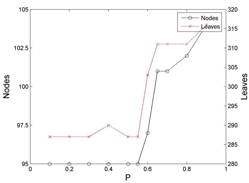
Figure 5. Relationship diagrams of the classification performance
performance of the decision tree of the Balance
dataset and the location of the entropy kernel peak. (a) Relationship between the accuracy rate and
entropy kernel
kernelpeak
peak location;
location; (b) Relationship
(b) Relationship between
between theand
the scale scale and kernel
entropy entropy
peakkernel peak
location.
location.where nf is the number of samples that tested unsuccessfully in the test set, and
4. Decision
precision Tree
is the Learning
degree Algorithm
of accuracy Based
of a test seton Constraint
except Gain
to testing and Depth Optimal
failures.
4.1. Evaluation of the Attribute Selection Based on Constraint Gain and Depth Induction
5.2. Influence of the Entropy Peak Shift to Decision Tree Learning
Considering a node of the decision tree, its corresponding training dataset is S = {Y1 , Y2 , ..., Yn },
In this study, we initially conducted an experiment on the influence of the peak shift of the
in which the attribute variable set of a dataset is {X1 , X2 , ..., Xm }, the class tag of each sample is Ti ∈C,
constraint entropy on decision tree learning. The experiment used the training and test sets of
and C is the class set of the things. Thus, each sample, Yi , consists of the attributes and a class tag, Ti .
Balance, Tic-Tac-Toe, and Dermatology. The experiment result is presented in Figure 5 Figure 6
According to the Gain principle [22], we aim to find the attribute of a strong gain in the training dataset,
Figure 7.
S, whilst the impact of attribute otherness is reduced. Therefore, we defined the entropy estimation of
For the Balance training set, the training of a decision tree is implemented by moving the peak
gain uncertainty measured on the basis of the peak-shift as follows:
of the constraint entropy as the probability ranges from low to high for the heuristic, namely, SP∈
[0.1, 0.9]. The accuracy rate of the classification, Acc,v exhibits a tendency of initially increase and
then decrease. Amongst the GCE ( XAcc
areas, Es (C | X ja) =
j ) =presents ∑ distribution
high | Xsection
P( X ji ) Hsc (Cat ji ) [0.1, 0.7] and a sudden (7)
i =1
low distribution at section [0.8, 0.9] until it reaches the lowest value, in which Acc is relatively
steadyGCE
where at section
is the [0.1,
gain 0.55], but appears
constraint entropy to be protruding
estimation, whichpartially
is measuredat sections [0.35,
by the key 0.45] and
changed [0.575,
part from
0.625].
the GainInformula,
addition,inthe numbers
which of nodes and
the uncertainty measureleavesof of
thethe decision
category tree (Size) in
distribution arethe
relatively
attributelow at
space
section [0.1,
is Hsc , and Hsc0.55] and highby
is optimized atthe
section [0.6, 0.9]
constraint entropyuntilbased
the highest distribution
on the peak-shift. Its is reached.
specific With the
calculation is
exception of the strong
expressed in Formula (8): local expressions at sections [0.35, 0.45] and [0.575, 0.625], the numbers of
nodes and leaves in other regions exhibit the opposite change distribution.
Figure 6 illustrates the training case of|Cthe |
Tic-tac-toe dataset. The general form of the decision
Hsc (C | X ji ) = ∑ P(Ck | X ji ) Isin ( P(Ck | X ji ), v) (8)
tree, Acc, exhibits an initially high and then low distribution; that is, it presents a relatively high
k =1
where P(Ck |Xji ) is the probability of distribution of a class, Ck , in the Xji value domain of an attribute,
Isin (P(Ck |Xji ), v) is an entropy kernel calculated specifically in accordance with either Formula (5) or (6).
Given the attributes set of the training dataset, S, the GCE measure is performed in accordance
with Formula (7). From this condition, we aim to find an attribute variable of the smallest uncertainty
of a class distribution in the attribute space, as defined in Formula (9):
A∗ = arg min{ GCE( X j )| j ∈ [1, | X |]} (9)
Xj ∈X
where A* is a set of candidate attributes that provide a partitioning node, in which the number of
values for each attribute is greater than 1.
Whilst evaluating the selection of attributes on the basis of the gain uncertainty formed by the
constraint entropy, we must consider the inductive convergence of the branches generated by a selected
split attribute to reduce the effects of samples and noise. We assume that the attribute, Xj , is selected as
a splitting attribute of the node for the decision tree induction. Given that the attribute’s, Xj , valueEntropy 2019, 21, 198 8 of 17
distribution is {Xj1 , Xj2 , ..., Xjv }, the dataset, S, is divided into v subsets and downward v branches.
Correspondingly, when an attribute, Xk (Xk 6= Xj ), is selected as a further split attribute in the subset of
the branches, the convergence branching number under the depth generated by the current tree node
attribute, Xj , is measured as follows:
kv
Bconv ( X j ) = ∑ Fl (Xjl ) + ∑ ∑ Fq (Xkq ) (10)
l ∈V i ∈U q = 1
where V is a set of branch sequence numbers that can be converged as the leaf by the attribute, Xj ,
and U is a set of branch sequence numbers that can be divided further into nodes by an attribute,
Xj . By contrast, Xjl and Xkq (q∈[0, kv], kv is the number of Xk values) are the attribute values of
the current tree node and the sub-branch node, correspondingly. Fl is the functions that determine
whether the branches of the attribute value of the current tree node is a leaf, and Fq is the functions that
determine whether the branches of the attribute value of the sub-branch node are a leaf. If P(Cb |Xjl ) = 1,
and P(Cb |Xkq ) = 1, where b∈[1, |C|], then, Fl and Fq are 1; otherwise, 0. Thus, Bconv (Xj ) is the strength
index, which measures the convergence of a branch at two inductive depths generated by the split
attribute, Xj , of the current tree node.
Similarly, when we select an attribute, Xj , as a split attribute of the current node for the decision
tree, we can expect to estimate the divergence of branches produced in-depth by Xj . Therefore, the split
attribute of a branch node generated by the division of attribute Xj is assumed to be Xk (Xk 6=Xj ).
Then, the number of fan-outs under the depth generated by the current tree node attribute, Xj ,
is measured as follows:
v kv
Bdiver ( X j ) = Nj ( X j ) + ∑ ∑ Nk (Xk ) (11)
i =1 q =1
where Nj is the number of branches generated by the current tree node, and Nk is the number of
branches generated by the subordinate node of a branch of the current tree node. Thus, Bdiver (Xj ) is the
aided index that measures the divergence of the branch at the two inductive depths produced by the
splitting attribute, Xj , of the current tree node.
4.2. Learning Algorithm Based on Constraint Gain and Depth Induction for a Decision Tree
According to the Hunt principle and the above-mentioned definition, this study proposed an
inductive system that is the heuristic framework of an optimal measure of a category convergence in
the attribute space. In this attribute space, minimal uncertainty distribution is searched based on the
constraint mechanism of the strength and summit, and constitutes the decision tree learning algorithm
(CGDT) of the constrained gain heuristic. Moreover, whilst GCE is used as the main measurement
index, the branch convergence, Bconv , and branch fan-out, Bdiver , are applied to be auxiliary indices
among the similar attributes of GCE. We aim to select split attributes of a strong deep convergence and
weak divergent, and form the constraint gained and depth inductive improved decision tree learning
algorithm (CGDIDT).
Therefore, the learning algorithm based on the constraint entropy for the decision tree designed is
defined specifically as follows (Algorithms 1 and 2):
In the algorithm presented above, Leaftype(S) is the function of a leaf class judgment,
and Effective(S) is the processing function to obtain a valid attribute set of the dataset, S. The complexity
of the entire CGDT(S, R) is the same as that of the ID3 algorithm. The core of the algorithm is the
attribute selection heuristic algorithm based on GCE.
The pruning of the above algorithms is turned off. The branch convergence and fan-out index
under the depth are introduced to optimize the learning process of the decision tree on the basis of
Algorithm 1.Entropy 2019, 21, 198 9 of 17
Algorithm 1. The learning algorithm of the constraint gained decision tree, CGDT (S, R).
Input: Training dataset, S, which has been filtered and labelled.
Output: Output decision tree classifier.
Pre-processing: For any sample in the dataset, {Y1 , Y2 , ..., Yn }: Yi = {X, Ti }, Ti ∈C to obtain the discrete training set.
Initialization: The training set, S, is used as the initial dataset of the decision tree to establish the root node, R,
which corresponds to the tree.
1. If Leaftype(S) = Ck , where Ck ∈C and k∈[0, |C|], then label the corresponding node, R, of the sample set, S,
as a leaf of the Ck category, and return.
2. Return the valid attribute set of the corresponding dataset, S, of the node: Xe = Effective(S). If Xe is an empty set,
then the maximal frequentness class is taken from the S set, and the node is marked as a leaf and is returned. If Xe
is only a single attribute set, then this attribute is returned directly as the split attribute of the node.
3. For any attribute, Xi (i∈[0, |Xe |]), in the Xe set, perform calculations on GCE. The attribute of the minimum
uncertainty is selected as the split attribute, A*, of the current node, R.
4. The dataset, S, of the current node, R, can be divided into v subsets, {S1 , S2 ..., Sv }, which correspond to the
attribute values, {A1 , A2 , ..., Av } of A*.
5. For i = 1, 2, ..., v
v CGDT(Si , Ri ).
Algorithm 2. Constraint gained and depth inductive decision tree algorithm, CGDIDT (S, R).
Input: Training dataset, S, which has been filtered and labelled.
Output: Output decision tree classifier.
Pre-processing: As Algorithm 1.
Initialization: As Algorithm 1.
1. Judge whether the Leaftype(S) = Ck (Ck and S definition is the same as in Algorithm 1), the corresponding
node, R, of the sample set, S, is labelled as a leaf of the Ck category when it is true, and return.
2. Return the valid attribute set of the corresponding dataset, S, of the node: Xe = Effective(S). If Xe is an empty
set, then the maximum frequency class is taken from the S set. The node is marked as a leaf and is returned.
If Xe is only a single attribute set, then return the attribute directly as the split attribute of the node, R.
3. Establish an empty set, H, for the candidate split attributes; firstly, obtain the attribute with the smallest
constraint gain, f, from the set, S, that is, f = Min{GCE(Xi ), i∈[0, |Xe |]}. Secondly, determine the candidate
attributes in which GCE is the same or similar to the minimum value, such as GCE≤(1 + r)f, where r∈[0, 0.5];
these candidate attributes are placed in the set, H.
4. Face the candidate attributes set, H, of the current node, and calculate the depth branch convergence number,
Bconv , and depth branch fan-out number, Bdiver , of each attribute. If the attribute with the optimal Bconv is not
the same as the GCE minimal attribute in the set, H, then select the attribute of the larger Bconv and smaller
Bdiver as the improved attribute. If the attribute obtained the optimal Bconv , and the GCE minimal attribute is
the same attribute in the set, H, then the split attribute, A*, selection is all with the GCE minimum evaluation as
the preferred attribute selection criteria for the current node and even the subsequent branch node.
5. Divide the dataset, S, of the current node, R, into v subsets, {S1 , S2 ..., Sv }, which correspond to the attribute
values, {A1 , A2 , ..., Av } of A*.
6. For i = 1, 2, ..., v
CGDIDT(Si , Ri ).Entropy 2019, 21, 198 10 of 17
5. Experiment Results
5.1. Experimental Setup
In this section, we use the 11 discretized and complete datasets of the UCI international machine
learning database as the original sample sets to verify the performance of the CGDT and CGDIDT
algorithms. The details of the datasets are provided in Table 1.
Table 1. Experimental datasets from the UCI machine learning repository.
No. Dataset Instances Attributes Num (A.v.) Range Distribution of Attributes (n/v) Num. of Class values Distr. of Class
1 Balance Scale 625 4 5~5 4/5 3{288,49,288}
2 Breast 699 9 9~11 1/9, 7/10, 1/11 2{458,261}
3 Dermatology 366 33 2~4 1/(2,3), 31/4 6{112,61,72,49,52,20}
4 Tic-Tac-Toe 958 9 3~3 9/3 2{626,332}
5 Voting 232 16 2~2 16/2 2{124,108}
6 Mushroom 8124 22 1~12 1/(1,7,10,12), 5/2, 4/4, 2/5, 2/6, 3/9 2{4208,3916}
7 Promoters 106 57 4~4 57/4 2{53,53}
8 Zoo 101 18 2~6 15/2, 1/6 7{41,20,5,13,4,8,10}
9 Monks1 * 124+308 6 2~4 2/2, 3/3, 1/4 2{62,62}
10 Monks2 * 169+263 6 2~4 2/2, 3/3, 1/4 2{105,64}
11 Monks3 * 122+310 6 2~4 2/2, 3/3, 1/4 2{62,60}
Note: Sign “Num(A.v.) range” denotes range of number of attribute values, “{ }” denotes the number of samples
for a class. Sign “n/v” denotes the number n of attributes for same values number v. Sign * denoted datasets are
training datasets of Monk as the original samples set.
Firstly, the representative Balance, Tic-Tac-Toe and Dermatology datasets were selected for the
peak shift experiment to observe the effects of the peak movement of the entropy core on decision
tree learning. For the first two datasets, the numbers of the attribute values are 5 and 3, respectively,
in which their numbers of the attributes values are the same in each dataset. For the subsequent
dataset, the numbers of the attributes values are mostly 4, except for two attributes for which the
numbers of the values are 2 and 3. The category distributions are Balance: {217, 39, 182}, Tic-Tac-Toe:
{439, 232}, and Dermatology: {74, 43, 53, 35, 39, 12}. Regardless of whether from the distribution of
the number of attributes values or the distribution of the sample categories, these three datasets are
highly representative for the peak shift effect experiment of the constraint entropy. The similar details
of other datasets are shown as Table 1.
Then, the CGDT and CGDIDT algorithm experiments were performed separately on the
11 datasets using the experimental system designed in this study. However, the ID3 and C4.5 (J48)
decision tree algorithms were implemented as references by the Weka system. The same training and
test sets were used for the experiment on different algorithms when the same dataset experiments were
performed on two different systems. Before the experiment, the dataset was sampled uniformly and
unrepeatably in accordance with the determined proportion, α, in which the extracted parts constituted
the training set and the remaining parts constituted the test set for learning, training, and validation.
In this study, a sampled proportion of α = 70% was first used for the training set. Even for the Monks
datasets, which provided the training sets, this learning experiment still used only α proportional
extracted datasets from the provided training set as learning training sets to verify the adaptability of
the learning algorithm, whereas all the remaining datasets were used for testing.
The classifier scale (Size) of a decision tree on the training set, the accuracy (Acc) for verifying the
test set, the F-measure, and the test coverage (Cov) were the indicators used to compare and evaluate the
algorithms in the experiment. The description of the specific indicators is given Equations (12) and (13):
nc
Acc = · 100%, Size = Ns + Ls (12)
nt
where nc is the number of samples that have been validated in the test set, nt is the total number of
tested samples, Ns is the number of nodes of the decision tree that are learnt and obtained in theEntropy 2019, 21, 198 11 of 17
training set, and Ls is the number of leaves of the decision tree that are learnt and obtained in the
training set.
2Acc · precision nt − n f nc
F-measure = , Cov = , precision = (13)
Acc + precision nt nt − n f
where nf is the number of samples that tested unsuccessfully in the test set, and precision is the degree
Entropy 2019, 21, x FOR PEER REVIEW 12 of 18
of accuracy of a test set except to testing failures.
Entropy 2019, 21, x FOR PEER REVIEW 12 of 18
distribution
5.2. Influenceatof section [0.1,Peak
the Entropy 0.7],Shift
in which it maintains
to Decision a period of high value at section [0.25, 0.35],
Tree Learning
and then demonstrates a low distribution at section [0.8, 0.9], with a steep decline at section > 0.8.
distribution at section
In thisthe
study, we [0.1, 0.7],conducted
initially in which itan maintains
experimenta period
on the of high value of at section [0.25,of
0.35],
However, numbers of nodes and leaves of the decision treeinfluence
(Size) exhibitthe
a peak
stableshift the
low-value
and then demonstrates
constraint entropy a low
on decision distribution at section [0.8, 0.9], with a steep decline at section > 0.8.
distribution at section [0.1, 0.7],tree learning.
which The an
indicates experiment
improvedused the training
reverse and test
distribution withsets
Acc.of Balance,
However, the
Tic-Tac-Toe, and numbers of nodes
Dermatology. Theand leaves of
experiment the is
result decision
presentedtreein(Size) exhibit
Figures 5–7. a stable low-value
distribution at section [0.1, 0.7], which indicates an improved reverse distribution with Acc.
(a) (b)
(a)
Figure 6. Relationship diagrams of the classification performance of the (b)
decision tree of the Tic-tac-
toe dataset and the location of the entropy kernel peak. (a) Relationship between the accuracy rate
Figure 6. Relationship
Relationship diagrams
diagramsof ofthe
theclassification
classificationperformance
performanceofof the decision
the tree
decision of of
tree thethe
Tic-tac-toe
Tic-tac-
and entropy kernel peak location; (b) Relationship between the scale and entropy kernel peak
dataset
toe andand
dataset the location of the
the location of entropy kernel
the entropy peak.peak.
kernel (a) Relationship between
(a) Relationship the accuracy
between rate and
the accuracy rate
location.
entropy kernel peak location; (b) Relationship between the scale and entropy kernel
and entropy kernel peak location; (b) Relationship between the scale and entropy kernel peak peak location.
location.
(a) Relation between accuracy rate and entropy kernel (b) Relation between scale and entropy kernel peak
peak location location
(a) Relation between accuracy rate and entropy kernel (b) Relation between scale and entropy kernel peak
Figure 7. Relationship diagrams
diagrams ofof the
peak location
Relationship the classification
classification performance
performance of
of the decision
decision tree
location
the tree of
of the
Dermatology dataset and the location of entropy kernel peak.
Figure 7. Relationship diagrams of the classification performance of the decision tree of the
Dermatology dataset and the location of entropy kernel peak.
For the Balance
Similarly, for the training set, the training
Dermatology trainingofset,
a decision tree isform
the general implemented by moving
of the decision tree,the peak
Acc, of
also
the constraint
displays entropy high
an initially as theand
probability
then low ranges from low tothat
distribution; highis,foritthe heuristic,
first achieves namely, SP∈[0.1,high
a relatively 0.9].
Similarly, for the Dermatology training set, the general form of the decision tree, Acc, also
The accuracyatrate
distribution of the
section classification,
[0.1, 0.3], and thenAcc,exhibits
exhibitsa alowtendency of initially
distribution and an increase
apparentandhollow
then decrease.
bucket
displays an initially high and then low distribution; that is, it first achieves a relatively high
Amongst
shape the areas,
at section Acc
[0.4, presents
0.9], in whicha high distribution
section [0.1, 0.3]atissection [0.1, high
the stable 0.7] and a sudden
section of Acc,low distribution
whereas sectionat
distribution at section [0.1, 0.3], and then exhibits a low distribution and an apparent hollow bucket
section
[0.45, [0.8,is0.9]
0.55] theuntil
lowestit reaches
section.the lowest value, in
Simultaneously, thewhich Acc isofrelatively
numbers nodes and steady
leavesat of
section [0.1, 0.55],
a decision tree
shape at section [0.4, 0.9], in which section [0.1, 0.3] is the stable high section of Acc, whereas section
but appears
(Size) display to be protruding partially
a considerably reverseatdistribution
sections [0.35,with0.45] andwhich
Acc, [0.575,is0.625].
low atIn section
addition,[0.1,
the numbers
0.3], but
[0.45, 0.55] is the lowest section. Simultaneously, the numbers of nodes and leaves of a decision tree
of nodes
high and leaves
at section [0.4,of0.9].
the decision
However, tree (Size) are relatively
a stronger volatility low at sectionwhich
is achieved, [0.1, 0.55] and high
is lowest at aatlow
section
SP
(Size) display a considerably reverse distribution with Acc, which is low at section [0.1, 0.3], but
[0.6, 0.9] until the highest distribution
section and highest at a high SP section. is reached. With the exception of the strong local expressions at
high at section [0.4, 0.9]. However, a stronger volatility is achieved, which is lowest at a low SP
The preceding analysis implies that although the Balance and Tic-tac-toe training sets with the
section and highest at a high SP section.
same number of attribute values exhibit a better stability distribution of classification performance
The preceding analysis implies that although the Balance and Tic-tac-toe training sets with the
and size than the Dermatology training set, which has a different number of attribute values, they
same number of attribute values exhibit a better stability distribution of classification performance
all have the same volatility and regularity is evident. That is, the Balance set at section [0.1, 0.3], Tic-
and size than the Dermatology training set, which has a different number of attribute values, they
tac-toe set at section [0.25, 0.35], and Dermatology set at section [0.1, 0.3] demonstrate improved
all have the same volatility and regularity is evident. That is, the Balance set at section [0.1, 0.3], Tic-Entropy 2019, 21, 198 12 of 17
sections [0.35, 0.45] and [0.575, 0.625], the numbers of nodes and leaves in other regions exhibit the
opposite change distribution.
Figure 6 illustrates the training case of the Tic-tac-toe dataset. The general form of the decision
tree, Acc, exhibits an initially high and then low distribution; that is, it presents a relatively high
distribution at section [0.1, 0.7], in which it maintains a period of high value at section [0.25, 0.35],
and then demonstrates a low distribution at section [0.8, 0.9], with a steep decline at section > 0.8.
However, the numbers of nodes and leaves of the decision tree (Size) exhibit a stable low-value
distribution at section [0.1, 0.7], which indicates an improved reverse distribution with Acc.
Similarly, for the Dermatology training set, the general form of the decision tree, Acc, also displays
an initially high and then low distribution; that is, it first achieves a relatively high distribution at section
[0.1, 0.3], and then exhibits a low distribution and an apparent hollow bucket shape at section [0.4, 0.9],
in which section [0.1, 0.3] is the stable high section of Acc, whereas section [0.45, 0.55] is the lowest section.
Simultaneously, the numbers of nodes and leaves of a decision tree (Size) display a considerably reverse
distribution with Acc, which is low at section [0.1, 0.3], but high at section [0.4, 0.9]. However, a stronger
volatility is achieved, which is lowest at a low SP section and highest at a high SP section.
The preceding analysis implies that although the Balance and Tic-tac-toe training sets with the
same number of attribute values exhibit a better stability distribution of classification performance and
size than the Dermatology training set, which has a different number of attribute values, they all have
the same volatility and regularity is evident. That is, the Balance set at section [0.1, 0.3], Tic-tac-toe set
at section [0.25, 0.35], and Dermatology set at section [0.1, 0.3] demonstrate improved agreement in
terms of the accuracy rate with the numbers of nodes and leaves. The details of which are as follows:
(1) For the Tic-tac-toe set with the same number of attribute values and a similar proportion of
sample categories, the accuracy rate and size (numbers of nodes and leaves) exhibit the best expression
for the decision tree when the peak of the entropy core, SP, is constrained at P = 1/3.
(2) For the Balance set with the same number of attribute values and a slightly different proportion
of sample categories, the corresponding numbers of nodes and leaves present the most stable expression
when SP is constrained at P = 1/5, although the accuracy rate of the decision tree does not reach the
maximum value.
(3) For the Dermatology set with different attribute values and a similar difference in the
proportion of samples categories, the corresponding numbers of nodes and leaves are small when SP
is constrained at P ≤ 1/4, whereas the accuracy rate of the decision tree is high.
The experiment on the three representative datasets shows that uncertainty is measured by the
constraint entropy, which consists of the dynamic peak shift of the entropy core in accordance with SP
= 1/v. Enhancing the rationality of split attribute selection is effective for decision tree induction.
5.3. Effects of Decision Tree Learning Based on Constraint Gain
In accordance with the rules obtained from the preceding experiment on the peak shift of
the entropy core, the constraint entropy of improved dynamic peak localization is determined.
Its contribution constitutes the GCE heuristic and it realizes the decision tree algorithm based on
constraint gain heuristic learning, CGDT. In this section, 11 datasets were used to compare the Gain
and Gainratio heuristics (pruning off). The experimental results are presented in Table 2.Entropy 2019, 21, 198 13 of 17
Table 2. The experimental results of decision tree Learning based on constraint gain.
Dataset Method Size Ns Ls Acc
Balance Scale Gain 388 97 291 43.8503
Gainratio 393 98 295 43.8503
GCE (CGDT) 382 95 287 46.5241
Breast Gain 78 13 65 89.0476
Gainratio 107 19 88 86.6667
GCE (CGDT) 87 16 71 87.1429
Dermatology Gain 64 20 44 93.6364
Gainratio 159 51 108 72.7273
GCE (CGDT) 58 20 38 96.3636
Tic-Tac-Toe Gain 255 92 163 81.1847
Gainratio 418 157 261 69.6864
GCE (CGDT) 269 98 171 83.6237
Voting Gain 27 13 14 94.3662
Gainratio 29 14 15 97.1831
GCE (CGDT) 27 13 14 95.7747
Mushroom Gain 29 5 24 100
Gainratio 45 9 36 100
GCE (CGDT) 35 6 29 100
Mushroom ** Gain 30 5 25 99.8031
Gainratio 48 9 39 99.8031
GCE (CGDT) 34 6 28 99.9508
Promoters Gain 30 8 22 71.8750
Gainratio 30 8 22 68.7500
GCE (CGDT) 29 8 21 75.0000
Zoo Gain 23 9 14 93.3333
Gainratio 23 9 14 90.0000
GCE (CGDT) 19 7 12 100
Monks1 * Gain 58 21 37 77.5974
Gainratio 52 19 33 83.1169
GCE (CGDT) 58 21 37 78.2468
Monks2 * Gain 109 43 66 53.6122
Gainratio 116 48 68 55.1331
GCE (CGDT) 108 42 66 55.8935
Monks3 * Gain 27 11 19 90.3226
Gainratio 25 11 21 94.1935
GCE (CGDT) 35 11 19 90.3226
Gain 98.9091 29.9091 69 80.8023
Average Gainratio 127 40 87 78.3007
GCE (CGDT) 100.6364 30.6364 70 82.6265
Note: The sign ‘**’ denotes the sampling proportion α = 50%, and its results are not considered in the average
calculation. The sign ‘*’ is the same of Table 1.
Firstly, the classification results of the decision tree are observed. The classification accuracy rate,
Acc, of the GCE heuristic is better than those of the Gain and Gainratio heuristics in eight and seven
datasets, respectively. The difference range of the former was 0.6494–6.6667%, and the mean value was
2.7464. That of the latter was 0.4762–23.6363%, and the mean value was 8.2477. In other datasets, GCE
has two datasets with the same Acc as that of the Gain heuristic, and another dataset with a weaker
Acc than that of the Gain heuristic, but stronger than that of the Gainratio heuristic. The difference
range is 0%—−1.905%, and the mean is −0.605. Meanwhile, GCE has one dataset with the same Acc
as that of the Gainratio heuristic, whereas the other three datasets are poor. The difference range is
0%–−4.8701%, and the mean is −2.5373. Accordingly, the classification Acc of only four datasets of the
Gainratio heuristic are better than that of the Gain heuristic.
Secondly, the size of the decision tree classifier is observed. The GCE heuristic has five datasets
with a smaller decision tree classifier than that of the Gain heuristic and nine datasets with a smaller
decision tree classifier than that of the Gainratio heuristic. The decision tree classifiers of the otherEntropy 2019, 21, 198 14 of 17
datasets are the same or close to one another. The Gainratio heuristic has two datasets with smaller
decision tree classifiers than those of the Gain heuristic. The other datasets have decision tree classifiers
that are considerably larger than those of the Gain heuristic.
For the larger Mushroom dataset, the learning experiment of reducing the sampling proportion
to 50% was conducted. The classification accuracy, Acc, of the GCE heuristic is better than those of
the Gain and Gainratio heuristics. The size of the decision tree classifier is larger than that of the Gain
heuristics and smaller than that of the Gainratio heuristic.
From the overall average of all the datasets, the numbers of branch nodes (30.6364) and leaves (70)
of the GCE heuristic are extremely close to those of the Gain heuristic (29.9091, 69) and considerably
less than those of the Gainratio heuristic. Meanwhile, the average size of the GCE heuristic’s decision
tree classifier is close to that of the Gain heuristic. The average accuracy of the GCE heuristic (82.6265)
is better than those of the Gain and Gainratio heuristics (80.8023 and 78.3007, respectively).
On average, the GCE heuristic based on the constraint entropy for a decision tree achieves better
classification accuracy than the Gain and Gainratio heuristics.
5.4. Effect of Optimized Learning of Combining Depth Induction
In the preceding section, the classifier for a decision tree is established through the inspired
learning of GCE in the CGDT algorithm. Its size characteristics show that the split attribute of tree
nodes should still be optimized in inductive convergence. CGDIDT is a learning algorithm of deep
induction optimization that is based on the GCE selection for a decision tree. It is compared with
ID3 and J48 of the Weka system. The experimental results are presented in Table 3.
The classification results of the CGDIDT decision tree demonstrate that the accuracy of
10 datasets is greater than that of the ID3 algorithm, with differences ranging from 1.4085 to 14.6104.
Meanwhile, one dataset is flat and the average difference is 4.7312. The size of nine datasets is less
than that of the ID3 algorithm, with a difference of −1–−104. The F-measure has 10 datasets that are
greater than the ID3 algorithm. Its coverage has eight datasets that are greater than the ID3 algorithm.
CGDIDT is also compared with the J48 algorithm. Its accuracy has five datasets that are better
than the average difference (8.3968), one dataset is flat and five datasets are weak (with an average
difference of −5.2556). Their average overall difference is 1.4278. Meanwhile, the size of 10 datasets
is bigger than that of J48. The F-measure has six better datasets, and its coverage has seven smaller
datasets and three flat datasets.
Finally, the J48 algorithm is compared with ID3. The accuracy has seven better datasets, one flat
dataset and five weak datasets. The average difference is 3.2854. Moreover, size has 11 smaller datasets.
The F-measure has seven better datasets, and its coverage has eight smaller datasets.
For the larger Mushroom dataset, the experimental results of reducing the sampling proportion
to 50% are as follows: The classification performance (Acc and F-measure) of the CGDIDT algorithm is
better than that of ID3 and the same as that of J48. Meanwhile, the size of CGDIDT is smaller than
those of ID3 and J48.
In conclusion, the classification accuracy and F-measure of the CGDIDT algorithm are averagely
better than those of the ID3 and J48 algorithms of the Weka system. The average classification
performance is further improved compared with that of CGDT. The average size and coverage of the
classifier is considerably improved compared with those of ID3. However, the classifier scale is weaker
than that of the J48 algorithm, which is the reason why the built-in pruning of J48 plays an evident role
in the Weka system.You can also read