The economic value of potential irrigation in Canterbury - Lincoln University
←
→
Page content transcription
If your browser does not render page correctly, please read the page content below
The economic value of potential irrigation in
Canterbury

Caroline Saunders
John Saunders

                                   September 2012

                               Lincoln University

                        i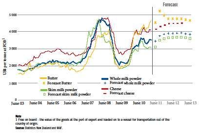
Contents

LIST OF TABLES                                       III
LIST OF FIGURES                                      IV
LIST OF ABBREVIATIONS                                V
EXECUTIVE SUMMARY                                     2
CHAPTER 1 INTRODUCTION                                3
       1.1   Irrigated land                           4
CHAPTER 2 BENEFITS OF IRRIGATION                     10
       2.1   Value of irrigation                     10
       2.2   Irrigation Valuation Model              13
       2.3   Value of different land uses            14
       2.4   Canterbury Economic Development Model   18
       2.5   Scenarios                               19
       2.6   Results by revenue and employment       21
       2.7   Effects on NZ                           24
       2.8   Conclusion                              29
REFERENCES                                           30
APPENDIX CANTERBURY AGRICULTURE                      31

                                            ii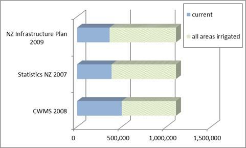
List of Tables
Table 1.1: Irrigable land (ha) by territorial authority and type (1)(2)(3)(4) (Year ended June)     4
Table 1.2: Summary of current irrigation in Canterbury by source                                    5
Table 1.3: Land use class of potentially irrigable land in Canterbury                               9
Table 2.1: Summary of assumed land-use (ha) for potentially irrigable land in Canterbury           11
Table 2.2: Land use on sampled farms                                                               12
Table 2.3: Revenue per hectare of land use                                                         14
Table 2.4: Land irrigated by scenario                                                              19
Table 2.5: Revenue effects for Canterbury by land use and scenario in 2031(NZD million)            21
Table 2.6: Total Revenue effects for Canterbury by land use and scenario in 2031 (NZD million)     21
Table 2.7: Employment effects for Canterbury by land use and scenario in 2031 (FTEs)               21
Table 2.8: Total employment effects for Canterbury by land use and scenario in 2031 (FTEs)         22
Table 2.9: Revenue effects for New Zealand by land use and scenario in 2031 (NZD million)          25
Table 2.10: Total revenue effects for New Zealand by land use and scenario in 2031 (NZD million)   25
Table 2.11: Employment effects for New Zealand by land use and scenario in 2031 (FTEs)             25
Table 2.12: Total employment effects for New Zealand by land use and scenario in 2031 (FTEs)       25
Table 2.13: Value added for Canterbury by land use and scenario in 2031 (million NZD)              27
Table 2.14: Total value added for Canterbury by land use and scenario in 2031 (NZD million)        27

                                                 iii
List of Figures
Figure 1.1: Potential irrigable area of Canterbury 6
Figure 1.2: NZLRI: Land use capability map 7
Figure 1.3: Land use capabilities of potentially irrigable land in Canterbury 8
Figure 1.4: Total irrigation, current and potential (ha) 9
Figure 2.1: LTEM projections of New Zealand producer prices (NZD/t) 15
Figure 2.2: Dairy export prices and MAF price forecast in US dollar terms 16
Figure 2.3: OECD projection of NZ dairy prices (NZD/t) to 2020 16
Figure 2.4: LTEM projection of NZ Dairy prices (USD/t) to 2020 17
Figure 2.5: Butter and cheese price comparison (USD/t) 17
Figure 2.6: Whole and skimmed milk powder price comparison (USD/t) 18
Figure 2.7: Assumed percentage distribution of land use of additional irrigated land in Canterbury 20
Figure 2.8: Total modelled irrigation (ha) by year and Scenario 20
Figure 2.9: Comparison of total revenue effects for Canterbury by land use and scenario in 2031 23
Figure 2.10: Comparison of employment effects for Canterbury by land use and scenario in 2031 23
Figure 2.11: Total additional revenue for Canterbury from each scenario 24
Figure 2.12: Total additional employment for Canterbury from each scenario 24
Figure 2.13: Comparison of total revenue for New Zealand by land use and scenario in 2031 26
Figure 2.14: Comparison of employment effects on New Zealand by land use and scenario in 2031 26
Figure 2.15: Comparison of total value added for Canterbury by land use and scenario in 2031 28
Figure 2.16: Total additional output (million NZD by scenario) in 2031 29
ivList of Abbreviations
CDC- Canterbury Development Corporation
CEDM- Canterbury Economic Development Model
CWMS- Canterbury Water Management Strategy
FAO- Food and Agriculture Organization of the United Nations
FTE- Full Time Equivalent
GIS- Geographic Information System
LRIS- Land Resource Information System
LTEM- Lincoln Trade and Environment Model
LUC- Land Use Capability
MAF- Ministry of Agriculture and Forestry
NZLRI- New Zealand Land Resource Inventory
OECD- Organisation for Economic Co-operation and Development
SMP- Skim Milk Powder
SONZAF- Situational and Outlook for New Zealand Agriculture and Forestry
WMP- Whole Milk Powder
v1
Executive Summary
The purpose of this report is to provide CDC with the ability to estimate the total benefits for
Canterbury and New Zealand from irrigation scenarios under the implementation of the Canterbury
Water Strategy.
This report describes a series of assumptions which under pin a model for valuing irrigation.
The model is built allowing different prices, uptake rates, irrigated area and different land
uses of irrigated land, to be defined.
The prices valuing land use are informed from both international and national data sources
and use the Lincoln Trade and Environment Model (LTEM) to allow the possibility of
different international policy market scenarios to be modelled.
Using these sources the model assigns values to different land uses under irrigation, and
projects price trends until to 2031.
The model gives final outputs in total revenue and employment effects from 2014 to 2031.
This includes the direct, indirect and induced effects by using the Canterbury Economic
Development Model.
The results presented here are based on a five year rate of uptake and predicted land uses
of irrigated area as 58 per cent dairy, 18 per cent irrigated sheep and beef, 20 per cent
arable and 3 per cent high-value arable.
Additionally irrigated land in all scenarios is assumed to have been previously utilised for
dryland sheep and beef farms.
Three modelled scenarios are covered in this report, based on GIS data describing the total potential
irrigable area of Canterbury, and a base current irrigation of 500,000 ha in Canterbury:
1. 607,773 ha additional irrigation, the upper bound of irrigation in Canterbury. All potential
irrigable land being irrigated.
2. 364,664 ha of additional irrigation, a more realistic estimate. 60 per cent of total potentially
irrigable land.
3. 250,000 ha of additional irrigation. An estimate of potential demand for irrigation taken
from the CWMS.
Total Effects by scenario, 2031
Revenue Employment Value Added
(million NZD) (FTEs) (million NZD)
Scenario Cant. NZ Cant. NZ Cant. NZ
Scenario 1 5070.07 7335.12 19106 20406 2710.68 3225.98
Scenario 2 3042.04 4401.07 11464 12244 1626.41 1935.59
Scenario 3 2085.51 3017.21 7859 8393 1115.00 1326.97
The results from the first scenario shows a total potential benefit of irrigation in Canterbury for New
Zealand, in 2031 of $7.3 billion and over 20,000 Full time equivalent (FTEs) jobs. The second, more
realistic scenario, showing a 60 per cent uptake of potential additional irrigable land irrigated netted
$4.4 billion in revenue and over 12,000 FTEs. Lastly the third scenario of projected demand from the
CWMS gave an additional $3 billion in revenue and over 8,000 FTEs.
2Chapter 1
Introduction
The purpose of this report is to provide CDC with estimates of the benefits for Canterbury from
irrigation with the implementation of the Canterbury Water Strategy. The report is based on a series
of assumptions underpinning a model for the valuation of irrigation. Flexibilities in the model allow
key assumptions to be changed and different scenarios to be valued.
Canterbury has abundant land, water and other natural sources in a benign and dry climate. The
region has a wide range of abundant natural resources with good fertile land and supply of high
quality water. Over 60 per cent of Canterbury land is capable of being cultivated, and Canterbury has
by far the highest share of New Zealand’s irrigated land. This abundance of resources enables a wide
range of rural activities including agriculture, viticulture and horticulture (see Appendix). Considering
the water demand and the water availability on an annual basis the Canterbury region has enough
water to meet its foreseeable abstractive needs and provide for in-stream flow requirements, but to
cope with the seasonal water demand the region has to have water storage.
The region is strategically located with good transport infrastructure, to support generic growth in
the agricultural sector, including the airport and the seaports. This is the strength of the region as it
allows importing and exporting both domestically and internationally at an affordable price.
Lyttelton and Timaru Ports are the two container ports of the region and therefore important for
Canterbury and for the South Island, especially for trade through the global transport network.
In terms of the climate the seasons in Canterbury vary dramatically, and the climate is heavily
influenced by the Southern Alps to the west. Long dry spells can occur in summer, causing drought
conditions, and temperatures are highest when hot dry northwesterlies blow over the plains.
Summer temperatures are often cooled by a northeasterly sea breeze, and the typical maximum
daytime summer air temperature ranges from 18°C to 26°C. Snow is common in the mountain
ranges during winter and the typical maximum daytime winter air temperature ranges from 7°C to
14°C.
The Canterbury Plains are dry which makes agricultural use difficult. The Plains are the largest
alluvial plains in New Zealand. They seem flat but they are a series of huge, gently sloping fans built
up by the major rivers (Malloy 1993). The substantial amount of water coming from the mountains
influences the area’s climate and land use. It also makes irrigation possible to achieve a successful
growth of a diversity of crops and pastures.
Productivity in Canterbury’s agricultural sector has grown consistently over the past years. In
particular the growth in the dairy sector has been significant over the past ten years, as shown in the
Appendix.
There have been various studies on the use and potential for the use of water in Canterbury and on
issues associated with this. In particular, in 2002, the Canterbury Strategic Water Study was
prepared by Lincoln Environmental for the Ministry of Agriculture and Forestry, Environment
Canterbury and the Ministry for the Environment (Morgan et al, 2002). The report began by
recognising that seventy per cent of New Zealand’s irrigated land is located in the Canterbury region,
as is 58 per cent of all water allocated for consumptive use in New Zealand. Canterbury is therefore
a very high user of water
31.1 Irrigated land
There is no definitive figure of current irrigated land in Canterbury, instead many estimates have
been put forward by various institutions. The government’s national infrastructure plan for 2011
states that the national level of irrigation is approximately 620,000 ha, with 520,000 being in the
South Island. The infrastructure plan from the previous year, put the estimated irrigated land in
Canterbury as of 2009 at 363,614 ha, up from 347,022 ha in 2000. In contrast, the CWMS put the
figure for irrigated area in Canterbury much higher at 500,000 ha as of 2008, making up for 70 per
cent of the country’s total (an increase from287,000 ha in 2002).
Table 1.3 shows a summary of irrigated land in the districts of the Canterbury Region and New
Zealand. This shows in Canterbury the highest population of land is irrigated by spray systems,
accounting 81.4 per cent, followed by 16.7 per cent which are irrigated by flood systems.
Table 1.1: Irrigable land (ha) by territorial authority and type (1)(2)(3)(4) (Year ended June)
Total area Irrigable area Irrigable Irrigable area Irrigable area
Territorial
equipped for by flood area by by micro with systems not
authority spray
irrigation systems systems specified
systems
Kaikoura 3,653 C 3,296 C C
Hurunui 30,042 9,107 18,991 1,519 1,042
Waimakariri 29,472 2,076 26,043 711 1,026
Christchurch City 7,083 C 6,050 268 234
Selwyn 84,450 5,793 75,617 1,146 3,246
Ashburton 140,163 30,450 108,033 626 3,166
Timaru 45,068 1,351 41,697 482 2,242
Mackenzie 4,952 1,270 8,798 C C
Waimate 29,197 9,626 18,738 111 1,004
Waitaki 36,248 8,957 24,739 1,154 2,525
Canterbury 385,271 64,386 313,710 5,734 13,237
South Island 522,168 108,103 384,773 25,629 23,524
New Zealand 619,293 110,917 456,705 41,657 34,653
Note:
(1) Figures may not add to the totals due to rounding.
(2) Land area could have been irrigated using existing resource consents and equipment on the farm.
(3) Irrigable area may be irrigated by more than one system.
(4) Some figures have been revised since the initial release of data in August 2008.
Symbols: C confidential
4Source: Statistics New Zealand (2007)
Table 1.2: Summary of current irrigation in Canterbury by source
Source Total ha irrigated
CWMS 2008 500,000
NZ Infrastructure Plan 2009 363,614
Statistics NZ 2007 385271e
Symbols: e area equipped for irrigation
Sources: Canterbury Water (2010), Treasury (2009), Stats NZ (2007)
From MAF estimates, of this irrigated area in Canterbury, 34 per cent is on dairy pasture, 36 per cent
other pasture, 27 per cent arable and less than 3 per cent on horticulture and viticulture (LE 2000).
Potentially irrigable land
Given the fact that the estimates of the current irrigated land in Canterbury are uncertain it is not
surprising that the potential irrigable land is also a contentious figure. Part of the difficulty of
answering this question is the definition of irrigable and how to include existing irrigable land which
benefits from more reliable irrigation. In this study as we are assessing the implementation for the
Canterbury Water Strategy. Even so this is still contentious especially relating to what is new
irrigated land.
The CWMS states that of a gross potentially irrigable area of 1.3 million hectares, 500,000 ha is
already irrigated. To further analyse this and the capabilities of the irrigable land this study has
drawn on a number of sources as reported below.
A 2002 study (Morgan et al. 2002) utilizing the Land Resource Information System (or LRIS, from
Landcare Research), a GIS database, and a set of inclusion criteria for land, found the gross potential
irrigable area in Canterbury to be 1,296,371 ha. This number was reduced to 1,002,420 ha after
allowances for land-use for housing, shelter belts and other non-irrigated uses. This is a high
estimate, which included major forested areas and made no exclusions based on soil suitability, and
can be seen therefore as an upper bound figure for irrigation in Canterbury.
Figure 1.2 below is the map of the potentially irrigable areas of Canterbury, from the LRIS. The shows
the total land in Canterbury with a slope of 15 degrees or less, the inclination upon which irrigation
can take place. Of this total area several further exclusion criteria were enforced. All urban and river
areas were taken out. Also areas with unsuitable soil types for irrigation, high rainfall (over 1200
mm/yr), smaller isolated areas and areas above 600m were not included. This area of 1,296,371 was
used as the basis for total irrigation in the possible irrigation valuation model in this study.
5Figure 1.1: Potential irrigable area of Canterbury
The next task is to determine how much of the total area given by the LRIS potentially irrigable map
of Canterbury, is appropriate for different land uses. For this purpose we utilized the land use
capability (LUC) classes from the New Zealand Land Resource Inventory (NZLRI) (Landcare 2012) as
seen in Figure 1.3. The land use capability classifications define land based on its ability to sustain
long-term production. It divides land into eight major classes indicating the land’s general ability to
sustain production, four sub-classes, which define the main limitation upon production within an
area (soil, erosion, wetness and climate), and finally adding a unit to group similar landscapes. The
eight LUC classes give the broadest description of suitability of land from various land uses, with LUC
1 being the most suitable class of land for sustained production, and LUC 8 being the least suitable
class, unsuitable for any arable and pastoral production. Furthermore, of these classes, LUCs 1-4 are
considered suitable for the production of arable crops, and LUCs 1-7 suitable for pastoral usage.
6Figure 1.2: NZLRI: Land use capability map
For this project we overlaid the map of LUCs with map of potentially irrigable areas of Canterbury, to find
which irrigable areas were suited to various land usages. The overlay is shown in Figure 1.4.
7Figure 1.3: Land use capabilities of potentially irrigable land in Canterbury
Table 1.5 shows the distribution of land given from the overlay of the two maps. As this table
illustrates the majority of irrigable land in Canterbury is either LUC class 3 or 4. As the map of
potentially irrigable area already applied certain critera much of the unsuitable land for production
has been previously excluded, thus only a small proportion of land falls into LUC 8 or any of the
other unsuitable land classes.
While under the definitions of LUCs the class LUC 4 is suitable, this is only a rank of low suitability,
with “severe physical limitations to arable use...[that]…substantially reduce the range of crops which
can be grown. (Lynn at el, 2009, p.58)”. As LUC 4 is not ideal land for all arable growth for the
purposes of modelling we have deemed only LUCs 1-3 as potential land for arable use, as to avoid
LUC 4 land un-suited to modelled crops or land which could only be worked infrequently due to
physical limitations. Similarly we have discounted LUC 7 as being unsuited to pastoral use with
irrigation. Whilst this land can potentially be pastoral, it’s limitations would make intensive pastoral
use difficult.
Therefore, in the model LUCs 1-3 are considered appropriate for arable use, and LUCs 1-6
appropriate for pastoral use. This gives a total potential area of 683,622 ha potential for arable, and
1,107,773 ha potential for pastoral, of which 424,150 ha is appropriate only for pastoral useages.
8Table 1.3: Land use class of potentially irrigable land in Canterbury
LUC Area (ha)
1 19864
2 243988
3 419768
4 414820
5 9329
6 144798
7 19349
8 2182
e 274
l 1217
r 16596
t 848
Notes: e,l,r,t: refer to areas of lakes, rivers and urban development
Source: Morgan et al. (2002)
Therefore, for this study we have used the total irrigable area possible in Canterbury at 1.1 million
hectares as the definitive figure. This includes existing area irrigated (0.5 million hectares) as we do
not know where the existing irrigation is taking place and on what classes of land. Figure 1.5 shows
the current area of irrigation as estimated by three sources, as part of the 1.1 million total
potentially irrigable land presented in this study. The figure of 1.1 million does not account for the
viability, either economically or in terms of physical supply, of irrigation in a particular area. Rather,
this figure expresses the potential of the land itself to support irrigation.
Figure 1.4: Total irrigation, current and potential (ha)
Sources: Canterbury Water (2010), Treasury (2009), Stats NZ (2007)
One limitation of the GIS approach to the problem of determining the land available for irrigation in
Canterbury is a lack of spatial data for the currently irrigated areas of Canterbury. Thus the
distribution of LUCs is assumed to be equal across currently irrigated and non-irrigated land, as the
irrigated land cannot be taken out of the mapped area, while accurately portraying the location of
areas with different LUCs.
9Chapter 2
Benefits of Irrigation
2.1 Value of irrigation
There have been numerous studies on the benefits of irrigation. To assess this requires key sources
of information including:-
1. The uptake rates over time for irrigation
2. The increased returns and value added from the change in land use
3. The changes in agricultural land use by type
4. The impact of this on the wider community
1. The uptake rates over time for irrigation
Of course the rate of uptake of any new irrigations scheme will affect the economic benefits from
the scheme. This will vary depending upon a variety of factors including land potential; the age of
the farmer; size of farm; investment required to develop the infrastructure for the irrigation and
alternative uses; market condition and alternative land uses among other factors. There have been
relatively few studies of uptake rates ex-post apart from the Opuha dam, (Harris et al 2006). There
have been a variety of surveys of farmers re their intentions when irrigation becomes available but
these are generally not in the public domain. The other source of information is the secondary data
sources of land use in Canterbury as shown in the Appendix. Whilst this cannot be related directly to
irrigation it does provide some context for uptake and land use.
In this study we have modelled two scenarios involving a 100 per cent and a 60 per cent uptake
targets. These have been assumed to be converted at 20 per cent per year thus taking five years to
achieve the assumed uptake rates.
2. The increased returns and value added from the change in land use
To estimate the benefits from irrigation it is important to assess the value of the irrigated activity
both in terms of total revenue and also value added. Again there have been a number of studies
which have estimated this. In most of these studies the values used have been derived from the
MAF Farm Monitoring Reports and the MAF (2004) report on the value of irrigation. These provide
information on the key value of outputs and inputs by sectors. This study therefore uses the latest
data available from the Farm Monitoring Reports but supplements these data with data from the
LTEM (Lincoln Trade and Environment Model), the OECD and other sources as mentioned. This
enables the impact of trade policy and changing world demand and supply conditions on prices to be
estimated.
3. The changes in agricultural land use type
The actual land uses to which farmers convert will depend on a variety of factors including
investment required, relative returns and their security, among others. Obviously the major land
use type over the last decade that farmers have converted to is dairy. To estimate value of irrigation,
therefore we need to estimate what farmers will convert their land use too.
10Morgan et al (2002) did estimate these, as shown in Table 2.1. This shows the potentially irrigated
areas categorized in six land use groups based on their water requirements. The total gross area of
potentially irrigable land in the Canterbury Region is estimated to be 1,296,361ha. It records that the
highest potential rate of the regions irrigated land is for intensive livestock/dairy support (46 per
cent) and for dairying (33 per cent).
Table 2.1: Summary of assumed land-use (ha) for potentially irrigable land in Canterbury
Land use category
Water Intensive Horticul- Forestry Total by
Resource livestock ture & Viti- & other resource
Area Dairying & dairy Arable Lifestyle processed culture non- area
support crops irrigated
Clarence 1,653 1,653 0%
100%
Coastal 8,297 5,981 14,278 1%
Kaikoura 58% 42%
Waiau 10,867 43,339 54,206 4%
20% 80%
Hurunui 21,601 26,616 9,085 6,414 63,716 5%
34% 42% 14% 10%
Ashley/ 52,306 18,447 16,977 87,730 7%
Waipara 60% 21% 19%
Waimakariri 18,975 34,186 2,196 26,647 6,501 11,352 99,857 8%
19% 34% 2% 27% 7% 11%
Selwyn 84,977 64,520 39,748 26,434 215,679 17%
39% 30% 19% 12%
Banks 5,993 6,678 12,671 1%
Peninsula 47% 53%
Rakaia 6,896 5,462 5,089 17,447 1%
40% 31% 29%
Ashburton 145,479 84,530 51,212 281,221 22%
52% 30% 18%
Rangitata 9,619 8,131 17,750 1%
54% 46%
Opihi-Orari 74,260 42,074 8,703 6,968 132,005 10%
56% 32% 7% 5%
Coastal Sth. 27,719 49,650 4,392 3,801 85,562 7%
Canterbury 32% 58% 5% 5%
Waitaki 22,904 176,574 13,118 212,596 16%
11% 6%
Total by 431,594 595,022 111,34 77,521 10,769 45,681 24,444 1,296,371 100%
land use 0
33% 46% 9% 6% 1% 3% 2% 100%
type
Source: Morgan et al. (2002)
11Another source of data on the potential land use changes was the study of the impacts the Opuha
Dam had on the surrounding economy and community showed the differences in land-use, between
comparable irrigated and dryland farms within the command area of the Opuha scheme. Seen in
Table 2.2, only farms with irrigation had land used for dairying, showing a changing land use away
from sheep and to a lesser extent beef towards dairy in the case of livestock farms. Farms with
irrigation also showed higher stocking rates. As for cropping, the total percentage of effective area
devoted to cropping was 10 per cent higher on farms with irrigation. While a smaller percentage of
this effective area was used for cereal grain, small seed and other crops, more was used on feed
crops and process vegetables relatively. The table shows smaller proportions of cropping area for
both cereal grain and other crops in irrigated farms, however interestingly due to the larger effective
area used for cropping, the total average hectares for cereal grain and other crops is higher than in
the dryland sample.
In this study the farms surveyed as ‘irrigated’ had a total of 5,129 Ha irrigated out of a total 10,410
Ha effective area, leaving slightly under half of the total effective land un-irrigated. Thus whilst Table
2.2 shows considerable changes in land-use, there would be expected a larger shift towards dairy,
vegetables and crops, and away from sheep and beef as seen, if the total effective area was
irrigated. The relatively low proportion of potential land actually irrigated may reflect the fact the
study was completed only a short time after the scheme was finished.
Table 2.2: Land use on sampled farms
Dryland Irrigated
Proportion of Pastoral Stock units %
Sheep 75% 44%
Beef 18% 12%
Dairy 0% 35%
Deer 8% 9%
Stocking Rate on Effective Area (su / ha) 9.0 9.9
Stocking Rate on Livestock Area (su / ha) 11.4 13.7
Proportion of Cropping Area
Feed crops grown for sale 2% 9%
Cereal grain area 53% 38%
Process Vegetable area 3% 23%
Small seed area 28% 23%
Other crop area 15% 7%
Crop as a % Effective Area 15% 25%
Horticulture, Viticulture and Other 15%
Source: Harris et al. (2006)
4. The impact of this on the wider community
The benefits of irrigation are of course not just on farm but encompass the wider community. Again
there have been a number of studies which have estimated this. The CWMS estimated that irrigated
land in Canterbury is estimated to contribute $800 million net at farm gate to the national GDP and
1.1. billion of exports in 2007/08 (CWMS, 2009).
In a study looking into the impacts of the Opuha Dam on the provincial economy and community,
the total revenue was found to be 2.4 times as high (at $2,073/ha) for irrigated farms than dry land
farms (at $862/ha) (Aoraki Development Trust, 2006). Additionally, irrigated farms were found to
generate 2.0 times as many jobs, 2.3 times as much value added and three times as much household
income per hectare compared to dryland farms (Aoraki Development Trust, 2006). At a community
12level, it was found that for every thousand hectares of irrigation there was $7.7 million in output, 30
FTE in employment, $2.5 million in value added and $1.2 million in household income (Aoraki
Development Trust, 2006).
These studies generally use input output tables to estimate these wider benefits. This approach will
also be taken by this study using the input output tables in the Canterbury Economic Development
Model as outlined in next section.
2.2 Irrigation Valuation Model
For the purposes of this project a model was developed in order to estimate the potential direct,
indirect, induced and total monetary and employment effects a change in land-use associated with a
further irrigation of Canterbury would yield. The model projects these impacts out to 2031, with the
use of projected prices from the Lincoln Trade and Environment Model (LTEM), based on current
commodity prices informed from MAF Farm monitoring reports among other sources as identified
where used. The model is also calibrated to allow various levels of irrigation and different
proportions of types of land-use to be specified, allowing various farmer uptakes and land-use
scenarios to be modelled.
The area of irrigable land is a variable in the model which can be adjusted to various scenarios. For
this project the figure obtained through cross referencing the LRIS and NZLRI GIS land maps, was
1,107,773 hectares. As this area is further divided to express the suitability of land for arable and
pastoral use, a constraint was added to the model to restrict the total areas within the total irrigable
land that could be used for arable.
.
132.3 Value of different land uses
There is a large range of agricultural land-uses that would benefit under irrigation, so rather than to
exhaustively explore all possible options for irrigated land, four farm types were chosen, based on
the practically of implementation in Canterbury and the availability of data. These farm types are
dairy, sheep and beef, arable (grain) and high value arable (representing high value arable and
horticulture). In the model, the potential irrigable land in Canterbury is assigned across these farm
types depending on the scenario. It is also assumed that potentially irrigable land is converted from
dryland sheep and beef farming.
The value for each potential land-use under irrigation was determined by multiplying average
production figures with average commodity prices. Production figures were sourced from the
Canterbury model farm in MAF’s Farm Monitoring Reports in the case of dairy, sheep and beef
farming. As the required production data for arable crops is not available from the Farm Monitoring
report, arable production is taken instead from average national yields sourced from the OECD
agricultural stat database.
Current price data was obtained similarly from MAF’s Farm Monitoring Reports for all pastoral
commodities, and from the OECD for arable statistics. Prices for dairy, for example, were taken from
the Canterbury model farm in MAF’s Dairy monitoring reports to most accurately describe
Canterbury dairy. The price of 718 (c per milksolid) in 2010 was used, giving an average return per
hectare of Dairy of 8550 in the same year.
Table 2.4 shows the valuation of each land use as given by the model for the base year 2010.
Table 2.3: Revenue per hectare of land use
Revenue Value Added
Dryland Land Use Source(s)
(NZD/ha) (NZD/ha)
Sheep & Beef 634 290 Price adjusted MAF estimates
Irrigated Land Use
Dairy 8550 4157 MAF Dairy Monitoring report
Sheep & Beef 1527 889 Price adjusted MAF estimates
Arable OECD Ag. Outlook & MAF arable
3029 1499
monitoring reports
High Value Arable 8000 3451 …
Price projections for all commodities were modelled in the LTEM up to the year 2020. The LTEM is a
partial equilibrium trade model focusing on the agricultural sector. The framework of the LTEM has
20 agricultural commodities and 21 countries, giving a comprehensive map of global agricultural
trade. The LTEM simulates global trade, consumption and production of agricultural commodities
out to the year 2020. As part of this simulation the LTEM derives national commodity prices for all
modelled goods. These projected commodity prices from the LTEM were used in this project to
provide an informed future value for farmed commodities in New Zealand. Figure 2.1 illustrates
these price projections from the LTEM for a few relevant commodities.
14Figure 2.1: LTEM projections of New Zealand producer prices (NZD/t)
3000
2500
2000
Wheat
1500 Beef
Sheep
1000
Milk
500
0
As the LTEM only projects prices to the year 2020, further external projections to the year 2031 were
made, based on the trends shown from the LTEM. These secondary projections from 2021 to 2031
were made by mapping the trend in prices from the base year (2008) to the final projected year
(2020) from the LTEM, and extrapolating the prices to 2031 based on the observed trend. The final
year of 2031 was selected to coincide with models based on census data.
While the price projections informing the model are taken from the LTEM, the yield and production
data in the irrigation valuation model are static from the base year (2010). The prices in the model
follow modelled trends, however, the potential changes in levels of production from land do not.
Thus the model does not account for any changes in stocking rates, yields or increased production
from changing technology, farm methods or systems which may occur within the timeframe of the
model.
The below three Figures: 2.2-4, show price projections for NZ dairy products from three different
sources: MAF’s SONZAF report, the OECD-FAO Agricultural outlook (OECD/FAO 2010) and the LTEM
respectively. All figures show the spike in dairy prices from 2008. The secondary spike in price
beginning in 2010 shown in the MAF and the OECD’s data is not seen in the LTEMs projection due to
its earlier base year of 2008, where the MAF and OECD projections are simulated from 2010. In the
long term however, all models forecast dairy prices dropping from this 2010 high. The MAF forecast
is relatively short term only projecting to 2013; while the OECD shows a slight recovery for dairy
prices in the long-term after a sharp decline from 2012 to 2014. The LTEMs projections show a
downward trend of NZ dairy prices, matching the long term projections from MAF and the OECD,
even with the earlier base year as described previously.
15Figure 2.2: Dairy export prices and MAF price forecast in US dollar terms
Source: MAF (2011)
Figure 2.3: OECD projection of NZ dairy prices (NZD/t) to 2020
7000
6000
5000 Butter (product weight)
4000 Cheese (product weight)
3000
Skim milk powder (product
2000 weight)
Wholemilk powder (product
1000 weight)
0
2003
2004
2005
2006
2007
2008
2009
2010
2011
2012
2013
2014
2015
2016
2017
2018
2019
2020
Source: OECD-FAO (2010)
16Figure 2.4: LTEM projection of NZ Dairy prices (USD/t) to 2020
4500
4000
3500
3000
Butter
2500
Cheese
2000
WMP
1500
1000 SMP
500
0
2001
2019
2000
2002
2003
2004
2005
2006
2007
2008
2009
2010
2011
2012
2013
2014
2015
2016
2017
2018
2020
To further compare the different models, Figures 2.5 and 2.6 show projections from the LTEM and
the OECD alongside each other. While the LTEM shows a simplified trend in comparison to the
OECDs Agricultural Outlook the long term trends are comparable, the LTEM’s projections for dairy in
2020 being no more than 20 per cent different from the OECDs. For Dairy, with the exception of
butter, the LTEM’s prices are higher than the OECDs, due to the high dairy price in the LTEMs base
year: 2008. The LTEM’s valuations for dairy can then be seen as optimistic in comparison to the
OECD’s projections. The advantage of linking to the LTEM is the ability to model future changes.
Figure 2.5: Butter and cheese price comparison (USD/t)
4500
4000
Butter LTEM
3500
Cheese LTEM
3000
2500 Butter OECD
2000 Cheese OECD
1500
2015
2003
2004
2005
2006
2007
2008
2009
2010
2011
2012
2013
2014
2016
2017
2018
2019
2020
Source: MAF (2011)
17Figure 2.6: Whole and skimmed milk powder price comparison (USD/t)
4500
4000
WMP LTEM
3500
SMP LTEM
3000
WMP OECD
2500
SMP OECD
2000
1500
2003
2004
2005
2006
2007
2008
2009
2010
2011
2012
2013
2014
2015
2016
2017
2018
2019
2020
Source: MAF (2011)
2.4 Canterbury Economic Development Model
The model uses the methods previously discussed to project the value of land under various land-
use changes in Canterbury. It gives these figures for both revenue and employment. These are
further divided into three categories, direct, indirect and induced, detailing the upstream effects a
change in land-use would produce.
The upstream effects illustrate the effects of one sector on another by measuring the
interdependences between a sector and the remaining economy. To measure these effects, the
model uses value–added and employment multipliers supplied by the CEDM. The Input/Output table
shows the input and output flows for a given sector and the remaining sectors in the economy. Thus,
a given sector may require inputs from several other sectors. Therefore, in measuring a change in
one sector, the interrelatedness between the sectors’ dictates that a proportional change must
occur in the related sectors. Through this concept, multipliers provide the relative effect of one
sector on another. The multipliers incorporate the direct, indirect and induced inputs on the
Canterbury economy. These inputs relate to total returns, value-added and employment.
The upstream effects are divided into three categories: direct, indirect and induced. Each of these
categories is described below.
The direct effects describe the total change in output and employment, experienced by the farms
due to the addition of irrigation and the change of land-use. In the case of revenue this is calculated
as the total annual value of produce on the land under the new irrigated land-use, with the annual
value of the baseline sheep and beef pastoral farming subtracted to show the increased value gained
with irrigation rather than the total value of farms under irrigation. The change in employment
shows the increased farm related employment associated with the increased revenue.
Indirect effects show the revenue and employment benefits experienced by secondary firms and
sectors which supply the primary farms implementing irrigation. The increased revenue produced by
the direct effects, creates a larger demand for secondary sources which facilitate and supply the
farms, sources such as transport, farm management consultancy and the like. It is the changes in
revenue and employment in the suppliers of these input goods and services that are quantified in
the indirect effects.
18Lastly, induced effects are the wider impacts on revenue and employment in the local area, created
with the increase in household income and expenditure from the direct and indirect effects. These
encapsulate changes in spending resulting from the direct and indirect effects, for example with
increased revenue on farm, a farmer will then spend more at his local store perhaps. The changes in
direct and indirect effects flow on to affect the wider community due to changed spending.
Thus the model produces the total direct, indirect and induced changes in revenue and employment
as a result of irrigation and land-use changes. The analysis does exclude downstream benefits such
as an increase in processing. These could be estimated on an ad hoc basis but there is no consistent
methodology to assess their total amount.
2.5 Scenarios
Three scenarios were specifically modelled for this report. The first assumed the total potentially
irrigable area of 1,107,773 ha irrigated, demonstrating the maximum potential impacts of irrigation
in Canterbury, based on the estimate of 500,000 ha of currently irrigated land in Canterbury, this
first scenario then models an additional 607,773 ha of irrigation. The second scenario gives a more
conservative estimate, of a 60 per cent uptake (364,664 ha additional) giving a total of 864,664 ha
irrigated. The third and last scenario is based on a Canterbury Water Management Strategy
projection of an additional 250,000 ha of potential irrigation in Canterbury (Canterbury Water 2012),
this scenario then gives 750,000 total hectares irrigated in Canterbury. Each scenario is presented
below in Table 2.5.
Table 2.4: Land irrigated by scenario
Additional irrigation
Scenario Total irrigation (ha) Description
(ha)
Base level N/A 500,000 Current Irrigation
100% of potential
Scenario 1 607,773 1,107,773
additional irrigation
60% of potential
Scenario 2 364,664 864,664
additional irrigation
CWMS projected
Scenario 3 250,000 750,000
potential irrigation
For all scenarios it was assumed that land use changes would primarily turn to dairy and dairy
support as evidenced in the Ophua dam study and the CWMS’s assumed land-use for Canterbury,
with some pastoral non-dairy remaining. We have thus split the irrigated area into 58 per cent dairy,
18 per cent irrigated sheep and beef, 20 per cent arable and 3 per cent high-value arable.
19Figure 2.7: Assumed percentage distribution of land use of additional irrigated land in Canterbury
3
20 Dairy
Sheep & Beef
Arable
18 58
High Value Arable
The implementation and uptake of new irrigation schemes can vary greatly depending on the
circumstances of new irrigation schemes. As this study deals with the total irrigable land in
Canterbury, rather than relating to any particular proposed irrigation scheme a five year uptake rate
was assumed. Irrigation is implemented then gradually over this five year period as shown in Figure
2.8.
Figure 2.8: Total modelled irrigation (ha) by year and Scenario
1200000
1100000
Scenario 1
1000000 Scenario 2
Scenario 3
900000
800000
700000
600000
500000
2028
2014
2015
2016
2017
2018
2019
2020
2021
2022
2023
2024
2025
2026
2027
2029
2030
2031
Base
202.6 Results by revenue and employment
The results showing the effects on revenue are presented in Tables 2.6 and 2.7. As expected, with
the majority of additional irrigated lands assigned to dairy support and production, dairying provides
the highest economic value through direct and indirect induced effects across all scenarios. The total
effects from dairy for the 100 per cent scenario are $4,178 million, for the 60 per cent scenario
$2,507 million and $1,718 million for the CWMS 250,000 hectare scenario. The next most valuable
land use is arable (assumed to account for 20 per cent of newly irrigated land) with total effects
reaching $456 million in the 100 per cent irrigated scenario, $274 million for the 60 per cent
scenario, and $188 million in the CWMS scenario.
Table 2.5: Revenue effects for Canterbury by land use and scenario in 2031(NZD million)
Direct effects Indirect & induced Effects
Scen. 1 Scen. 2 Scen. 3 Scen. 1 Scen. 2 Scen. 3
Dairy 2519.52 1511.71 1036.37 1658.17 994.90 682.07
Sheep & Beef 88.20 52.92 36.28 66.44 39.86 27.33
High Value Arable 151.49 90.90 62.31 130.02 78.01 53.48
Arable 241.32 144.79 99.26 214.91 128.94 88.40
Total 3000.54 1800.32 1234.23 2069.53 1241.72 851.28
Table 2.6: Total Revenue effects for Canterbury by land use and scenario in 2031 (NZD million)
Total Effects
Scenario 1 Scenario 2 Scenario 3
Dairy 4177.69 2506.61 1718.44
Sheep & Beef 154.64 92.78 63.61
High Value Arable 281.51 168.91 115.80
Arable 456.23 273.74 187.66
Total 5070.07 3042.04 2085.51
Interestingly, the value of direct effects and the indirect induced effects are very similar across all
industries and both scenarios. In all scenarios the direct effects account for 60 per cent of the value
for dairy, 57 per cent for sheep & beef, 53 per cent for high value arable and 52 per cent for arable.
Overall, the total direct, indirect and induced effects on revenue from all land changes for scenario 1
are $5,070 million, $3,042 million for the second scenario, and $2,086 million for the third scenario.
Table 2.7: Employment effects for Canterbury by land use and scenario in 2031 (FTEs)
Direct effects Indirect & induced Effects
Scen. 1 Scen. 2 Scen. 3 Scen. 1 Scen. 2 Scen. 3
Dairy 6899 4139 2838 8298 4979 3413
Sheep & Beef 239 144 98 329 198 135
High Value Arable 1273 764 524 686 411 282
Arable 349 210 144 1032 619 425
Total 8761 5256 3604 10345 6207 4255
21Table 2.8: Total employment effects for Canterbury by land use and scenario in 2031 (FTEs)
Total Effects
Scenario 1 Scenario 2 Scenario 3
Dairy 15197 9118 6251
Sheep & Beef 569 341 234
High Value Arable 1959 1175 806
Arable 1382 829 568
Total 19106 11464 7859
In respect to employment, as shown in Tables 2.8 and 2.9, given modelled assumptions the dairy
industry is again the largest provider of full time equivalent jobs with 6,899 direct full-time
equivalent employments, and 8,298 indirect and induced for the 100 per cent irrigation scenario,
4,139 direct FTEs and 4,979 indirect and induced FTEs for the 60 per cent scenario, and 2,838 direct
FTEs and 3,413 indirect and induced FTEs in the CWMS scenario. The next most valuable industry in
regards to employment is high value arable going by the total effects, but looking at the direct
effects and indirect and induced effects separately, a different story is shown. High value arable
provides the second highest, ‘direct’ FTEs for both scenarios but the arable industry provides the
second highest ‘indirect’ number of jobs across both scenarios. High value arable total effects are
1,959 FTEs for the 100 per cent scenario, 1,175 for the 60 per cent scenario, and 806 in the CWMS
scenario. Arable total effects are 1,382 FTEs for the 100 per cent scenario, 829 for the 60 per cent
scenario, and finally 568 for the CWMS scenario.
In contrast to revenue, the portion of jobs provided directly and indirectly across the industries for
both scenarios is mixed. Notably, for employment coming from the arable industry in the 100 per
cent scenario, only 25 per cent is direct effects. High value arable is at the other end of the scale
with 65 per cent provided from direct effects.
Given the assumed land uses, the modelling shows that sheep and beef provide the lowest direct
and indirect and induced effects across both revenue and employment in both scenarios.
The 100 per cent scenario produces total revenue effects across all land use changes in 2031 of $5
billion, almost 16,000 FTE jobs with full irrigation, while the more practical 60 per cent irrigation
scenario has a more modest $3 billion total revenue impact and creates over 9,500 FTE jobs. The
final CWMS 250,000 hectare scenario offers total revenue effects of over $2 billion and over 6,500
FTE jobs.
The comparisons in Figures 2.9 and 2.10 show the relative revenue and employment effects within
each land use between each scenario. These figures illustrate the differences in magnitude between
the scenarios, and the predominance of the effects from dairy in comparison to other land uses.
22Figure 2.9: Comparison of total revenue effects for Canterbury by land use and scenario in 2031
Indirect & induced Scen. 3
Arable Direct Scen. 3
Indirect & induced Scen. 2
Direct Scen. 2
High Value Arable
Indirect & induced Scen 1.
Direct Scen. 1
Sheep & Beef
Dairy
0 500 1000 1500 2000 2500 3000
NZD mil
Figure 2.10: Comparison of employment effects for Canterbury by land use and scenario in 2031
Indirect & induced Scen. 3
Arable Direct Scen. 3
Indirect & induced Scen. 2
Direct Scen. 2
High Value Arable
Indirect & induced Scen 1.
Direct Scen. 1
Sheep & Beef
Dairy
0 1000 2000 3000 4000 5000 6000 7000 8000 9000
FTEs
Figures 2.11 and 2.12 show the additional revenue and employment each scenario generates on top
of the revenue given by the current irrigated land in Canterbury.
23Figure 2.11: Total additional revenue for Canterbury from each scenario
Scenario 1
10000
Scenario 2
9000
Scenario 3
8000
Current irrigated
7000
NZD mil
6000
5000
4000
3000
2000
1000
0
Figure 2.12: Total additional employment for Canterbury from each scenario
Scenario 1
40000
Scenario 2
35000 Scenario 3
30000 Current irrigated
FTEs
25000
20000
15000
10000
5000
0
2.7 Effects on NZ
Tables 2.10 through 2.13 present the effects of the various scenarios on New Zealand as a whole.
The results show trends similar to the impacts on Canterbury. The total effects for the 100 per cent
24irrigation scenario are $7,335 million for New Zealand and over 20,000 FTEs. The 60 per cent
irrigation scenario has lesser effects with an increase of $4,401 million and about 12,000 FTEs. Lastly
the CWMS scenario yields effects for New Zealand of a total increase in revenue of $3,017 million
and over 8,000 FTEs. Of these effects dairy provides the largest benefit, accounting for about 80 per
cent of the total additional revenue and additional employment.
Table 2.9: Revenue effects for New Zealand by land use and scenario in 2031 (NZD million)
Direct effects Indirect & induced Effects
Scen. 1 Scen. 2 Scen. 3 Scen. 1 Scen. 2 Scen. 3
Dairy 2519.52 1511.71 1036.37 3571.45 2142.87 1469.07
Sheep & Beef 88.20 52.92 36.28 125.03 75.02 51.43
High Value Arable 151.49 90.90 62.31 226.72 136.03 93.26
Arable 241.32 144.79 99.26 411.39 246.83 169.22
Total 3000.54 1800.32 1234.23 4334.59 2600.75 1782.98
Table 2.10: Total revenue effects for New Zealand by land use and scenario in 2031 (NZD million)
Total Effects
Scenario 1 Scenario 2 Scenario 3
Dairy 6090.97 3654.58 2505.45
Sheep & Beef 213.23 127.94 87.71
High Value Arable 378.22 226.93 155.57
Arable 652.71 391.63 268.48
Total 7335.12 4401.07 3017.21
Table 2.11: Employment effects for New Zealand by land use and scenario in 2031 (FTEs)
Direct effects Indirect & induced Effects
Scen. 1 Scen. 2 Scen. 3 Scen. 1 Scen. 2 Scen. 3
Dairy 6899 4139 2838 9381 5629 3859
Sheep & Beef 239 144 98 450 270 185
High Value Arable 1273 764 524 1251 751 515
Arable 349 210 144 563 338 232
Total 8761 5256 3604 11645 6987 4790
Table 2.12: Total employment effects for New Zealand by land use and scenario in 2031 (FTEs)
Total Effects
Scenario 1 Scenario 2 Scenario 3
Dairy 16280 9768 6697
Sheep & Beef 689 414 284
High Value Arable 2524 1514 1038
Arable 913 548 375
Total 20406 12244 8394
25Figures 2.15 and 2.16 illustrate the comparative effects of Scenarios 1 and 2 on New Zealand. As can
be seen, with the assumed land uses entered into the model, dairy has the largest effect for New
Zealand. Interestingly, arable and high value arable have larger indirect and induced effects than
direct effects on employment.
Figure 2.13: Comparison of total revenue for New Zealand by land use and scenario in 2031
Indirect & induced Scen.
3
Arable Direct Scen. 3
Indirect & induced Scen.
2
High Value Arable Direct Scen. 2
Indirect & induced Scen 1.
Sheep & Beef
Dairy
0 500 1000 1500 2000 2500 3000 3500 4000
NZD mil
Figure 2.14: Comparison of employment effects on New Zealand by land use and scenario in 2031
Indirect & induced Scen. 3
Arable Direct Scen. 3
Indirect & induced Scen. 2
Direct Scen. 2
High Value Arable
Indirect & induced Scen 1.
Direct Scen. 1
Sheep & Beef
Dairy
0 2000 4000 6000 8000 10000
FTEs
26Results by value add
The benefits from irrigation were also calculated to assess their value added. Value added is the
difference between the total value of production and the cost of production. This was calculated
using the sources identified earlier in particular the MAF Farm Monitoring Reports and the MAF
(2004) study. The CEDM was then used to determine the upstream impacts. These results are
presented below.
As shown in Tables 2.14 and 2.15, dairy has the largest value added of all land uses, accounting for
almost 85 per cent of total effects in both scenarios. The total value added is $2.7 billion under the
100 per cent irrigated scenario and about $1.6 billion with only 60 per cent irrigation. The CWMS
scenario gives over $1.1 billion in value added.
Table 2.13: Value added for Canterbury by land use and scenario in 2031 (million NZD)
Direct effects Indirect & induced Effects
Scen. 1 Scen. 2 Scen. 3 Scen. 1 Scen. 2 Scen. 3
Dairy 1584.79 950.87 651.88 715.95 429.57 294.50
Sheep & Beef 28.51 17.10 11.73 28.61 17.16 11.77
High Value Arable 83.13 49.88 34.19 57.10 34.26 23.49
Arable 117.11 70.26 48.17 95.48 57.29 39.27
Total 1813.54 1088.12 745.98 897.14 538.29 369.03
Table 2.14: Total value added for Canterbury by land use and scenario in 2031 (NZD million)
Total Effects
Scenario 1 Scenario 2 Scenario 3
Dairy 2300.74 1380.44 946.38
Sheep & Beef 57.12 34.27 23.49
High Value Arable 140.24 84.14 57.68
Arable 212.59 127.55 87.45
Total 2710.68 1626.41 1115.00
Figure 2.17 illustrates the added value across the scenarios, with dairy having the largest impacts,
both direct, indirect and induced, by a large margin. The greatest value added being direct for dairy
in all scenarios
27Figure 2.15: Comparison of total value added for Canterbury by land use and scenario in 2031
Indirect & induced Scen. 3
Arable Direct Scen. 3
Indirect & induced Scen. 2
Direct Scen. 2
High Value Arable
Indirect & induced Scen 1.
Direct Scen. 1
Sheep & Beef
Dairy
0 500 1000 1500 2000
NZD mil
282.8 Conclusion
Total benefits of irrigation
This study estimates that the additional direct, indirect and induced effects across all land use
changes for the 100 per cent irrigated land scenario in 2031 are $5 billion in revenue, adding over
19,000 FTE jobs and $2.7 billion in value added with full irrigation, while the more practical 60 per
cent irrigation scenario gives a more modest $3 billion total revenue, over 11,000 FTE jobs and $1.6
billion in value added. The 250,000 scenario from the CWMS would give $2 billion, almost 8,000 FTEs
and $1.1 billion in value added. These figures represent the additional value of irrigating all areas of
Canterbury with land suitable to production under irrigation (in addition to the 500,000 hectares of
total existing irrigated land in Canterbury in the CWMS)
Figure 2.16: Total additional output (million NZD by scenario) in 2031
29References
Canterbury Water (2010). Canterbury Water Management Strategy. July.
Canterbury Water (2012). Potential Storage and Demand by Zone. May
Dark, A. (2008) Canterbury Strategic Water Study Stage 4: Meeting Potential Demand With Minimum
Storage Proceedings of the Irrigation New Zealand Conference, 13-15 October 2008. Christchurch,
New Zealand: Irrigation New Zealand Association.
Harris, S., G. Butcher and W. Smith (2006). The Opuha Dam: An ex post study of its impacts on the
provincial economy and community. August
Landcare Research. New Zealand Land Resource Inventory (NZLRI) Portal. Downloaded 26 June 2012
from http://lris.scinfo.org.nz/
Lincoln Environmental (2000). Information on Water Allocation in New Zealand Report for the
Ministry for the Environment. Report No. 4375/1. April.
Livestock Improvement Corporation (LIC) NZ Dairy Statistics 2007/ 2008 downloaded 3 March 2009
from http://viewer.zmags.com/publication/d159833c#/d159833c/1
Lynn, I.H., A.K. Manderson, M.J. Page, G.R. Harmsworth, G.O. Eyles, G.B. Douglas, A.D. Mackay and
P.J.F. Newsome (2009). Land Use Capability Survey Handbook- a New Zealand handbook for the
classification of land 3rd ed. Hamilton, Ag Research; Lincoln, Landcare Research; Lower Hutt, GNS
Science. 163p.
Ministry of Agriculture and Forestry (2011). Situation and Outlook for New Zealand Agriculture and
Forestry. June.
Molloy, L. (1993). Soils in the New Zealand Landscape. The Living Mantle (2nd ed.). Mallinson Rendel
Publishers Ltd., Wellington, in association with the New Zealand Society of Soil Science.
Morgan, M., V. Bidwell, J. Bright, I. McIndoe and C. Robb (2002) Canterbury Strategic Water Study.
Report for the Ministry of Agriculture and Forestry, Environment Canterbury and the Ministry for the
Environment, Report No 4557/1, Lincoln Environmental, Lincoln International.
New Zealand Government, Treasury (2009). Infrastructure: Facts and Issues: Towards the First
National Infrastructure Plan. September.
OECD/FAO (2010), OECD-FAO Agricultural Outlook: Highlights 2010, OECD Agriculture
Statistics (database), 10.1787/data-00500-en
Statistics New Zealand, Agricultural Production Census 2007, http://www.stats.govt.nz/tables/2007-
ag-prod/default.htm.
30Appendix
Canterbury Agriculture
A.1 Agriculture in Canterbury and its contribution to the NZ economy.
This section outlines agriculture and land use statistics of the Canterbury Region. Where
appropriate, it compares regional data with New Zealand data.
Comparisons of Canterbury’s farming patterns and land use can be made using Agricultural
Production Census (Statistics New Zealand 2002, 2007) and Agricultural Production Statistics data
(Statistics New Zealand, 2009). A high proportion of the land of the Canterbury region is devoted to
agricultural activities as shown in Table 1. Approximately 41 per cent of Canterbury is grassland and
another 41 per cent is tussock, with arable 6 per cent. This highlights the importance of the pastoral
sector to Canterbury, especially when compared to the rest of New Zealand.
Table 1: Land use in Canterbury and New Zealand, 2002 and 2007
(area in hectares at 30 June)
2002 2007
New
Canterbury New Zealand Canterbury Zealand
Tussock and danthonia used for grazing (whether
oversown or not) 1,372,793 3,322,224 1,324,288 2,900,463
Grassland 1,212,694 8,242,695 1,364,779 8,086,160
Grain, seed and fodder crop land, and land
prepared for these crops 205,724 424,466 205,636 367,404
Horticultural land and land prepared for
horticulture 12,267 109,397 16,770 132,892
Plantations of exotic trees intended for harvest 108,388 1,827,596 98,569 1,708,282
Mature native bush 58,200 483,465 65,251 448,247
Native scrub and regenerating native bush 103,444 789,735 98,674 625,981
Other land 77,381 390,306 109,789 431,467
Total Land 3,150,891 15,589,885 3,303,965 14,700,897
Source: Statistics New Zealand, 2007 Agricultural Production Census
The 2007 Agricultural Census shows land use in Canterbury divided by farm type. As Table 2 shows,
the large majority of farmed land in Christchurch (97 per cent) is used for livestock. Of this, 83 per
cent is used for sheep and/or beef farming, being the largest combined type of farming in
Canterbury by area, sheep farms accounting for the largest share of land use. Dairy farming accounts
for 7 per cent of total farming land-use in 2007, forestry only 1.45 per cent. Fruit, arable, viticulture
and all other farm types combined used one per cent of the total land use in Canterbury.
31You can also read