New Zealand Environmental Data Stack (NZEnvDS): A standardised collection of spatial layers for environmental modelling and site characterisation
←
→
Page content transcription
If your browser does not render page correctly, please read the page content below
McCarthy
New Zealand
         et al.:
             Journal
                 Environmental
                      of Ecology
                               spatial
                                 (2021)layers
                                         45(2):for3440
                                                   NZ © 2021 New Zealand Ecological Society.                                        1

                  RESEARCH

New Zealand Environmental Data Stack (NZEnvDS): A standardised collection of
spatial layers for environmental modelling and site characterisation

James K. McCarthy1* , John R. Leathwick2, Pierre Roudier3,4 , James R. F. Barringer1 , Thomas R. Etherington1                 ,
Fraser J. Morgan4,5 , Nathan P. Odgers1 , Robbie H. Price6 , Susan K. Wiser1 and Sarah J. Richardson1
1
  Manaaki Whenua – Landcare Research, Lincoln 7640, New Zealand
2
  john.leathwick@gmail.com
3
  Manaaki Whenua – Landcare Research, Palmerston North 4442, New Zealand
4
  Te Pūnaha Matatini, A New Zealand Centre of Research Excellence, Auckland 1142, New Zealand
5
  Manaaki Whenua – Landcare Research, Auckland 1072, New Zealand
6
  Manaaki Whenua – Landcare Research, Hamilton 3216, New Zealand
*Author for correspondence (Email: mccarthyj@landcareresearch.co.nz)

Published online: 18 June 2021

          Abstract: Environmental variation is a crucial driver of ecological pattern, and spatial layers representing
          this variation are key to understanding and predicting important ecosystem distributions and processes. A
          national, standardised collection of different environmental gradients has the potential to support a variety of
          large-scale research questions, but to date these data sets have been limited and difficult to obtain. Here we
          describe the New Zealand Environmental Data Stack (NZEnvDS), a comprehensive set of 72 environmental
          layers quantifying spatial patterns of climate, soil, topography and terrain, as well as geographical distance
          at 100 m resolution, covering New Zealand’s three main islands and surrounding inshore islands. NZEnvDS
          includes layers from the Land Environments of New Zealand (LENZ), additional layers generated for LENZ
          but never publicly released, and several additional layers generated more recently. We also include an analysis
          of correlation between variables. All final NZEnvDS layers, their original source layers, and the R-code used
          to generate them are available publicly for download at https://doi.org/10.7931/m6rm-vz40.
          Keywords: climate surfaces, environmental variables, geographical distance, landform, macroecology, open
          access data, terrain, topography, soil

Introduction                                                          potential forest distributions (Leathwick 2001), species refugia
                                                                      (Buckley et al. 2010, McCarthy et al. 2021), ecosystem services
The term macroecology was first used to describe the study            (Ausseil et al. 2013), production forest productivity (Palmer
of relationships between organisms and their environment at           et al. 2009), and forest carbon uptake (Whitehead et al. 2001).
large spatial scales by Brown and Maurer (1989). Since then,          One common feature across these studies, however, is their
the use of quantitative spatial data to explore and explain           reliance on high-quality, collated, and curated spatial data
ecological patterns has proliferated. Concurrent advances in          characterising the abiotic environment.
our ability to collect (e.g. iNaturalist; https://inaturalist.nz/),        Spatial layers used for environmental analyses typically
store (e.g. National Vegetation Survey Databank, https://nvs.         include some combination of variables describing climate,
landcareresearch.co.nz/; Wiser et al. 2001), and share (e.g.          soil, topography, and disturbance. These are commonly used
Global Biodiversity Information Facility; https://www.gbif.           for broad-scale predictions, or, in the absence of site-level
org/) biodiversity data; to describe the abiotic environment at       measurements, they can be used to derive values describing
fine scales (Viscarra Rossel & Bui 2016); and to interrogate          the abiotic conditions. Climate layers estimated using spatial
data sets of increasing size and complexity (Weigand et al.           interpolation methods, weather station data, and elevation
2020) have allowed ecologists to tackle analyses of ever-             data (Hutchinson 1995; Xu & Hutchinson 2010) are most
increasing complexity and geographical scope. While species           commonly used for this purpose (e.g. Richardson et al. 2004;
distribution models (SDMs) are probably the most common               Pawson et al. 2008) and can provide a more realistic value than
application of spatial analysis and prediction in ecology, other      one measured at the nearest weather station if this is located
spatial patterns are also analysed and explored along a similar       some distance away (Tait et al. 2012). Soil and disturbance
theme. Examples from New Zealand include investigations               variables can be more challenging to measure and project
of species richness patterns (Lehmann et al. 2002), forest            across large areas, but advances are being made, ranging
loss (Ewers et al. 2006; Walker et al. 2006; Perry et al. 2012),      from national contributions (McNeill et al. 2014; Viscarra
DOI: https://dx.doi.org/10.20422/nzjecol.45.31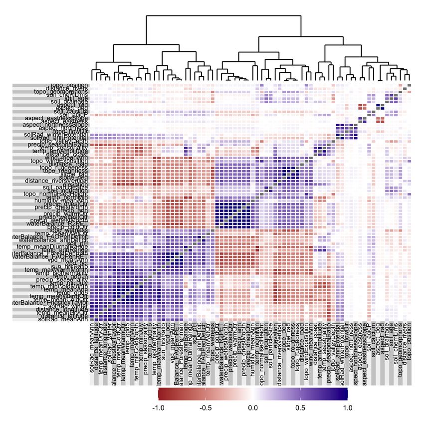
2                                                                              New Zealand Journal of Ecology, Vol. 45, No. 2, 2021

Rossel et al. 2015) to global initiatives (the Global Soil Map      New Zealand National Digital Elevation Model (NZDEM;
project; Arrouays et al. 2017). In recent decades, climate and      Barringer et al. 2002), which is also supplied (Appendix
soil variables have been supplemented with remotely sensed          S1). Additional variables have been derived from a range
variables from satellites, aeroplanes and drones, which capture     of New Zealand spatial data layers. The layers are ready to
spectral and structural attributes in ever-increasing resolution    use as input data in a range of environmental models and are
and extent (Verrelst et al. 2015). Variables can be continuous      available for download from the Manaaki Whenua – Landcare
(e.g. rainfall, temperature) or discrete (e.g. soil type); cover    Research DataStore at https://doi.org/10.7931/m6rm-vz40.
current, future or past time periods; and capture means,
extremes, seasonality, and variability at a range of resolutions
and extents. Individual variables can be highly correlated, but a   Methods
particular variable may be considered more proximally relevant
to a species’ ecology than a more commonly used, correlated         Source layers
alternative (Austin 2002). For example, when analysing the          The environmental layers provided here were largely derived
environmental variables driving the distribution of an alpine
                                                                    from previously unreleased layers generated as part of the
herb, mean minimum temperature of the coldest month may
                                                                    LENZ project (Leathwick et al. 2002a; Leathwick et al. 2002b).
be more appropriate than mean annual temperature, even
                                                                    Three of the geographical distance layers (horizontal distance
though these two predictors are highly correlated (Pearson’s
                                                                    to nearest river, distance to nearest road, vertical distance to
correlation = 0.89; Appendix S2 in Supplementary Materials).
                                                                    river) were derived using the LENZ spatial grids and shape
     Environmental spatial layers are most easily used when
                                                                    files downloaded from the Land Information New Zealand
they employ a consistent grid (of given resolution and extent)
                                                                    (LINZ) Data Service (Land Information New Zealand 2020b,
and projection system, allowing for easy extraction of point data
                                                                    2020c). The LENZ data included climate variables capturing
for model parameterisation and interpretation, and subsequent
                                                                    humidity, water balance, precipitation, solar radiation, sun hour
prediction. Although such layers are available at a global
                                                                    ratios, temperature, vapour pressure deficit, and wind speed;
scale (e.g. WorldClim, CHELSA), these initiatives are, by
                                                                    soil variables capturing phosphorous levels, calcium levels,
necessity of their coverage, constrained to a 1 km resolution
                                                                    age, drainage, induration (hardness), and particle size; and
(Hijmans et al. 2005; Karger et al. 2017). Over large parts
                                                                    slope. Many of the climate variables were originally presented
of New Zealand, complex topography and mountain ranges
                                                                    as annual values, but were, in fact, also generated monthly
produce steep gradients of climate and soil fertility that are
scarcely captured at a 1 km scale. A single 1 km grid square        (Leathwick et al. 2002b).
in the Southern Alps can span lowland rainforest to alpine               The LENZ climate layers were derived using ANUSPLIN
grassland (500–1200 m elevation), underscoring the need             software, which uses climate station and elevation data,
for finer-scale environmental spatial layers for ecological         and thin plate smoothing splines (Hutchinson & Gessler
modelling in New Zealand.                                           1994) to predict across an entire surface, in this case, all of
     In 2002 the Land Environments of New Zealand (LENZ)            New Zealand’s three main islands and surrounding inshore
was published, which included seven climate layers, seven soil      islands (Leathwick et al. 2002a). All climate data available
layers (ordinal categories), and a measure of slope (Leathwick      from the New Zealand Meteorological Service at the time were
et al. 2002a; Leathwick et al. 2003). These 15 layers were          included, primarily from the period 1950–1980. The LENZ soil
generated at 100 m resolution, downscaled to 25 m resolution,       layers were derived from the New Zealand Fundamental Soil
and used to classify New Zealand’s land environments. Several       Layers (FSL) (https://soils.landcareresearch.co.nz/soil-data/
additional climate layers were also generated as part of the        fundamental-soil-layers/; Newsome et al. 2008), which were
LENZ project, but did not inform the classification exercise.       themselves generated by expert interpretation of two major
The LENZ classifications and 15 environmental variables are         soil data sources: the New Zealand Land Resource Inventory
available online (at 25 m resolution; e.g. Land Information         (NZLRI), and the National Soils Database (NSD). While these
New Zealand 2020a), but the additional climate layers were          data sources suffer from inconsistencies and bias towards
never publicly released. While these layers have been used          lowland agricultural areas (see pp. 18–24 of Leathwick et al.
in spatial analyses (e.g. Watt et al. 2010; Perry et al. 2012),     2002a for a discussion of the LENZ soil layer reliability),
the number of climate variables available is much reduced           they remain the only spatially complete, quantitative layers
compared to modern standards (e.g. WorldClim; Hijmans               describing a range of soil properties for New Zealand. A recently
et al. 2005), and topographic variables (Amatulli et al. 2018)      released, quantitative layer describing soil pH between 0 and
are lacking.                                                        10 cm is also included (Roudier et al. 2020). The LENZ slope
     Here we describe Version 1.0 of the New Zealand                gradient layer was derived using 5 × 5 cell averaging filters
Environmental Data Stack (NZEnvDS), a package of 72                 from a 25 m digital elevation model (DEM), and resampled
environmental layers comprising 41 climate variables, eight         to 100 m (Leathwick et al. 2002a).
soil variables, 18 topographic/terrain variables, and six
geographical distance variables. Currently we do not include        Post processing
layers depicting land use and land cover, or remotely sensed        All data management and analyses were completed using R
variables depicting vegetation properties, but these could be       4.0.2 (R Core Team 2020) and the raster R package (Hijmans
included in future versions because they are known to be            2020), GRASS GIS version 7.8 (Neteler et al. 2012), and
good predictors of biodiversity patterns (Müller et al. 2015;       SAGA GIS version 7.3.0 (Conrad et al. 2015). Appendix S1
Dymond et al. 2019). Layers are provided at 100 m resolution        lists and describes the environmental layers, with details of
and comprise all the existing layers from LENZ, and additional      their derivation, and includes unmodified versions of the LENZ
layers calculated from the source climate variables, including      data layers. The full suite of 19 BIOCLIM variables were
equivalents to all 19 WorldClim variables. Topographic              calculated using monthly precipitation, minimum temperature,
variables have been derived from a 100 m version of the             and maximum temperature layers from LENZ, using the
McCarthy et al.: Environmental spatial layers for NZ 3
biovars function in the dismo R package (Hijmans et al. 2017); using the terrain function from dismo. A range of other terrain
however, two of the layers (mean annual temperature, bio1; total derivatives were generated in SAGA GIS from the NZDEM;
annual precipitation, bio12) were already included in LENZ, namely, the topographic wetness index (SAGA wetness index),
so we provide those original versions. Mean annual humidity, valley depth (a measure of vertical height below a summit),
mean annual daily sunshine ratio, annual water deficit, mean normalised height (a measure of position along a slope), and
annual vapour pressure deficit, and mean annual windspeed wind exposition. Other layers were derived from the NZDEM in
were calculated as the mean of their respective monthly GRASS GIS: annual and winter potential solar radiation using
LENZ layers. Normalised minimum winter temperature was the NZDEM and the r.sun.daily add-on (Petras et al. 2015),
calculated following Leathwick (2001) as the degree to which geomorphons using the r.geomorphon module (Jasiewicz et al.
winter temperatures vary from that expected based on their 2013; Jasiewicz & Stepinski 2013), and latitude and longitude
mean annual temperature. This layer provides a measure using the r.latlong module. Distance to coast, roads, and rivers
of continentality, with high values in oceanic (coastal and was generated using the distance function from raster. Vertical
mountainous) areas and low values in continental (lowland distance to river was calculated using the NZDEM and the
and interior) settings (Appendix S1). This layer has a very SAGA Channels module in SAGA GIS. Additional information
low correlation with many other commonly used temperature is provided in Appendix S1.
layers, such as mean annual temperature (Fig. 1; Appendix All layers were processed at the original LENZ grid
S2), allowing them to be used together in a model without resolution (100 m), and projection (New Zealand Map Grid;
confounding their relative effects (Leathwick 1995). Annual NZMG). Layers were also reprojected to New Zealand
temperature amplitude, another measure of continentality with Transverse Mercator (NZTM; see ‘Data accessibility’, below).
low values at the coast and high values in the interior (Appendix The original layers, source layers, and all code (R and Bash
S1), was calculated as the maximum monthly mean temperature scripts) used to generate the NZEnvDS layers are provided
minus the minimum monthly mean temperature. Two growing for reproducibility and to allow the community to generate
degree days layers (5°C and 16°C base) were calculated using additional layers from the source data. Since the NZEnvDS
the monthly minimum and maximum temperature layers layers have been generated and supplied with consistent
following the methods in Coops et al. (2001). We also include resolution and extent (Fig. 1), they are ready for use for these
a range of layers describing water balance (Appendix S1). types of analyses without the need for further processing.
A range of topographic/terrain indices and geographical Additional variables can, however, be created as required by
distances were generated using the NZDEM resampled at ecologists using the source layers, which are also supplied.
100 m resolution (Barringer et al. 2002; Land Information
New Zealand 2020d, 2020e). Measures of slope, aspect, Data accessibility
northness, and eastness (and also northness and eastness All source layers, the derived/final NZEnvDS layers, and the
incorporating slope gradient) were generated using the terrain scripts used to generate them are available for download from
function in the raster R package (Hijmans 2020), and following the Manaaki Whenua – Landcare Research DataStore (as TIFF
advice from Amatulli et al. (2018). Indices of topographic files in NZMG and NZTM projections), where they have been
position, roughness, and ruggedness, and the flow direction archived with a DOI: https://doi.org/10.7931/m6rm-vz40.
of water (see Appendix S1 for details) were also generated
(a) Mean annual (b) Soil (c) Topographic (d) Distance to
temperature (°C) particle size wetness index river (m)
15 14 50,000
V. large
Large 12
10 Moderate
Small 10 5,000
V. small 8
5
6
500
0
4
Figure 1. Example layers from the four broad environmental categories. (a) mean annual temperature (climate), (b) soil particle size
(soil), (c) topographic wetness index (terrain), and (d) distance to river (geographical distance). Note that distance to river (d) is presented
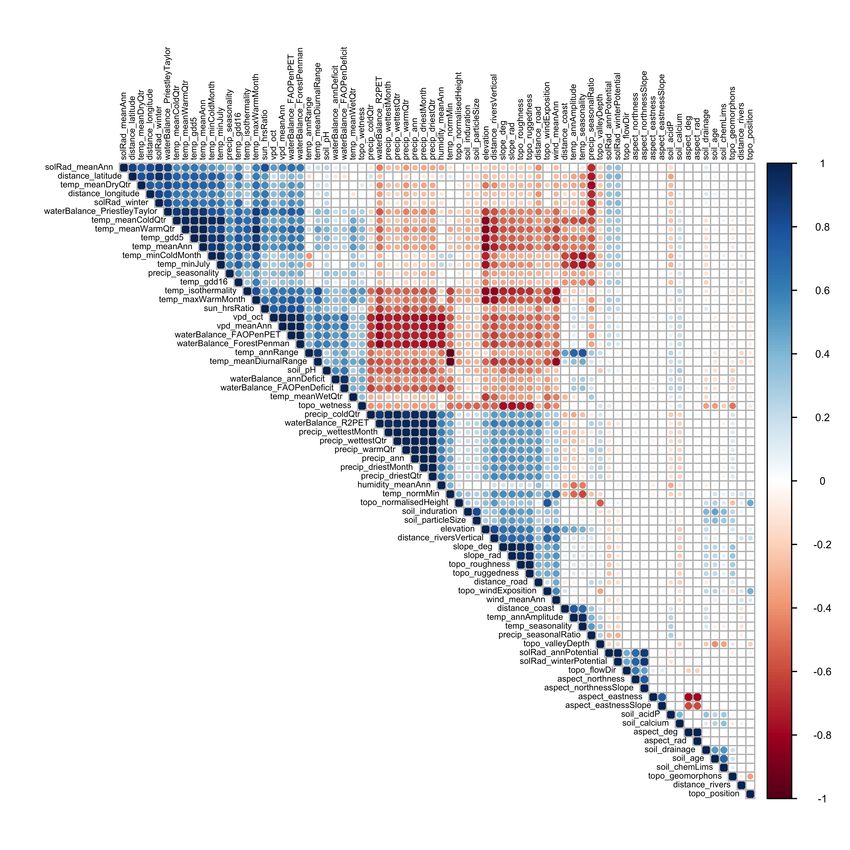
on a log10 scale to aid interpretation. Maps for all variables are included in Appendix S1.4 New Zealand Journal of Ecology, Vol. 45, No. 2, 2021 Figure 1. Pearson’s correlation coefficients between all 72 environmental variables. Correlation coefficients were estimated using values extracted from 50,000 random locations, and variables are grouped into related variables using Euclidean hierarchical clustering, based on their correlations using the superheat function from the superheat R package (Barter & Yu 2020). Full descriptions of all variables are included as Appendix S1, and correlation coefficient values are presented in Appendix S2.
McCarthy et al.: Environmental spatial layers for NZ                                                                                  5

Attribution                                                          explain the complicated disturbance and geological history
Please cite the original LENZ dataset (Leathwick et al. 2002a)       of the New Zealand landscape (glaciation, earthquake,
in addition to this article, to acknowledge the generation of        volcanic history, etc.) are lacking. These factors are known
many of the underlying data layers. When using the soil pH           to be important drivers of ecological processes and species
layer, please also cite Roudier et al. (2020).                       distributions, from fine spatial scales and decadal time scales,
                                                                     through to nationwide patterns over geological time scales
                                                                     (Wyse et al. 2018). For example, many tree species regenerate
Discussion                                                           on disturbed soils (e.g. mānuka Leptospermum scoparium;
                                                                     Stephens et al. 2005) or recent landslides (e.g. southern rātā
Collinearity and scale                                               Metrosideros umbellata; Stewart & Veblen 1982), yet spatial
                                                                     layers capturing these fine-scale disturbance events are
In any modelling framework using environmental variables             currently lacking, which has hampered efforts to predict the
such as those included on NZEnvDS, their selection and use           distributions of affected species (McCarthy et al. 2021). At
should be carefully considered (Williams et al. 2012). Many          larger temporal and spatial scales, New Zealand’s turbulent
of the variables included in NZEnvDS exhibit various levels          history of glaciation has left a strong imprint on the current
of Pearson’s pairwise correlation, ranging from 0.01 (e.g.           distributions of many plant and animal species. One example
mean monthly temperature range and degrees of latitude) to           is the discontinuous distribution of species present on the
0.99 (e.g. precipitation of the wettest month and total annual
                                                                     upper North and South Islands, but absent in between due
precipitation) (Fig. 2; Appendix S2). The inclusion of two or
                                                                     to the ancient separation of the two by a Pliocene sea strait
more collinear variables in a statistical model can result in
                                                                     (e.g. Quintinia serrata; McGlone 1985). Similar patterns are
unstable models and poor estimates of regression parameters
                                                                     observed in the South Island’s central Westland “beech gap”,
because it inflates their variance (Dormann et al. 2013). This
can lead to the inclusion of irrelevant predictors in a model,       a stretch of podocarp–broadleaf forest on the West Coast
which can be particularly problematic when extrapolating             flanked by beech forest to the north and south, likely to have
(Meloun et al. 2002). Colinear variables tend to be clustered        been driven by glaciation during the Last Glacial Maximum
into thematic groups such as precipitation, temperature, and         (and low levels of disturbance since; McGlone et al. 1996).
soil (Fig. 2), but variables within the same broad category can      The widely distributed rove beetle Brachynopus scutellaris
also be very weakly correlated. For example, mean temperature        is also largely absent from this gap (Leschen et al. 2008), and
of the coldest quarter and annual temperature variation share        also see Leathwick (1998) for an exploration of the effect
a Pearson’s correlation of only –0.10 (Appendix S2). A               of climate (using the layers provided here) on New Zealand
common threshold is to select variables with a correlation           beech gaps. Sourcing or generating layers describing these
6 New Zealand Journal of Ecology, Vol. 45, No. 2, 2021
climate data collected from 1950 to 1980 (Leathwick References
et al. 2002a). Layers characterising more recent climate
measurements (1981–2010) have been generated for Amatulli G, Domisch S, Tuanmu M-N, Parmentier B, Ranipeta
New Zealand, but these must be purchased, and were generated A, Malczyk J, Jetz W 2018. A suite of global, cross-scale
at a coarser 500 m resolution (NIWA 2021). While the LENZ- topographic variables for environmental and biodiversity
sourced layers were generated from older climate data, the modeling. Scientific Data 5: 180040.
relative magnitude of climate trends across the country and Arrouays D, Leenaars JGB, Richer-de-Forges AC, Adhikari K,
between locations remains relevant. They may also more Ballabio C, Greve M, Grundy M, Guerrero E, Hempel J,
closely match existing data records/observations, which often Hengl T, Heuvelink G, Batjes N, Carvalho E, Hartemink
represent historical collections of long-lived organisms (e.g. A, Hewitt A, Hong S-Y, Krasilnikov P, Lagacherie P,
multiple decades at least for shrubs and many herbaceous Lelyk G, Libohova Z, Lilly A, McBratney A, McKenzie
plants, centuries for trees). For example, plant observational N, Vasquez GM, Mulder VL, Minasny B, Montanarella L,
records from the New Zealand National Vegetation Survey Odeh I, Padarian J, Poggio L, Roudier P, Saby N, Savin
Databank (https://nvs.landcareresearch.co.nz/; Level 1 data) I, Searle R, Solbovoy V, Thompson J, Smith S, Sulaeman
and the New Zealand Virtual Herbarium Network have an Y, Vintila R, Rossel RV, Wilson P, Zhang G-L, Swerts M,
average collection year of 1976 (SD = 14.7 years) and 1967 Oorts K, Karklins A, Feng L, Ibelles Navarro AR, Levin
(SD = 33.7 years), respectively (analysis not shown), which A, Laktionova T, Dell’Acqua M, Suvannang N, Ruam W,
more closely match the LENZ climate layers than the more Prasad J, Patil N, Husnjak S, Pásztor L, Okx J, Hallett S,
recent layers. Updated layers covering time periods more Keay C, Farewell T, Lilja H, Juilleret J, Marx S, Takata
recent than those captured by LENZ would, however, be useful Y, Kazuyuki Y, Mansuy N, Panagos P, Van Liedekerke M,
for analyses of biotic invasions, shorter-lived species, and a Skalsky R, Sobocka J, Kobza J, Eftekhari K, Alavipanah
mechanistic understanding of species responses to climate SK, Moussadek R, Badraoui M, Da Silva M, Paterson
instability. As such, wider availability of more-recent climate G, Gonçalves MdC, Theocharopoulos S, Yemefack M,
surfaces should remain a priority. Tedou S, Vrscaj B, Grob U, Kozák J, Boruvka L, Dobos
Finally, technological advances mean that indices derived E, Taboada M, Moretti L, Rodriguez D 2017. Soil legacy
from remotely sensed data, primarily depicting vegetation cover data rescue via GlobalSoilMap and other international and
and growth (e.g. normalised difference vegetation index; NZVI) national initiatives. GeoResJ 14: 1–19.
but also forest structure and texture, are becoming increasingly Ausseil AGE, Dymond JR, Kirschbaum MUF, Andrew RM,
available. Satellite-based systems such as Landsat, Sentinel-2, Parfitt RL 2013. Assessment of multiple ecosystem services
GEDI and MODIS are readily available across various in New Zealand at the catchment scale. Environmental
temporal and spatial scales, and resolutions, and airborne Modelling & Software 43: 37–48.
LiDAR coverage is continually expanding. Furthermore, the Austin MP 2002. Spatial prediction of species distribution:
development and investigation of relationships between indices an interface between ecological theory and statistical
and biological processes is rapidly advancing (Xue & Su modelling. Ecological Modelling 157: 101–118.
2017). As these variables become even more commonly used Barringer JRF, Pairman D, McNeill SJ 2002. Development of
for environmental modelling, it will warrant further inclusion a high-resolution digital elevation model for New Zealand.
of such variables in future layer packages for New Zealand. Landcare Research Contract Report: LC0102/170.
Lincoln, New Zealand, Manaaki Whenua – Landcare
Research. 33 p.
Acknowledgements Barter R, Yu B 2020. superheat: A graphical tool for exploring
complex datasets using heatmaps. R package version 1.0.0.
Recent efforts to compile layers and write this manuscript Brown JH, Maurer BA 1989. Macroecology: The division
were supported by the Ministry of Business, Innovation of food and space among species on continents. Science
and Employment (MBIE; contract C09X1709) and MBIE’s 243: 1145–1150.
Strategic Science Investment Fund. We thank Matt McGlone Buckley TR, Marske K, Attanayake D 2010. Phylogeography
for suggesting inclusion of the annual temperature amplitude and ecological niche modelling of the New Zealand stick
layer, Rachelle Binny for help generating the growing insect Clitarchus hookeri (White) support survival in
degree day layers, and Ray Prebble for technical editing. The multiple coastal refugia. Journal of Biogeography 37:
manuscript was greatly improved following comments from 682–695.
two anonymous reviewers. Burnham KP, Anderson DR 2002. Model selection and
multimodel inference. New York, Springer. 488 p.
Bütikofer L, Anderson K, Bebber DP, Bennie JJ, Early RI,
Maclean IMD 2020. The problem of scale in predicting
Author Contributions biological responses to climate. Global Change Biology
26: 6657–6666.
JKM compiled the dataset, generated several layers, and wrote
Conrad O, Bechtel B, Bock M, Dietrich H, Fischer E, Gerlitz
the first draft of the manuscript; JRL and FJM generated the
L, Wehberg J, Wichmann V, Böhner J 2015. System
original LENZ layers, and contributed to revisions of the
for automated geoscientific analyses (SAGA) v. 2.1.4.
manuscript; PR generated several layers and contributed to
Geoscientific Model Development 8: 1991–2007.
revisions of the manuscript; JRFB, TRE, NPO, RHP, SKW,
Coops N, Loughhead A, Ryan P, Hutton R 2001. Development
and SJR all contributed to the conceptualisation of the data
of daily spatial heat unit mapping from monthly climatic
package, and revisions of the manuscript.
surfaces for the Australian continent. International Journal
of Geographical Information Science 15: 345–361.
Dormann CF, Elith J, Bacher S, Buchmann C, Carl G, CarréMcCarthy et al.: Environmental spatial layers for NZ 7
G, Marquéz JRG, Gruber B, Lafourcade B, Leitão PJ, New Zealand forest tree species. Journal of Vegetation
Münkemüller T, McClean C, Osborne PE, Reineking B, Science 6: 237–248.
Schröder B, Skidmore AK, Zurell D, Lautenbach S 2013. Leathwick JR 1998. Are New Zealand’s Nothofagus species in
Collinearity: a review of methods to deal with it and a equilibrium with their environment? Journal of Vegetation
simulation study evaluating their performance. Ecography Science 9: 719–732.
36: 27–46. Leathwick JR 2001. New Zealand’s potential forest pattern as
Dymond RJ, Zörner J, Shepherd DJ, Wiser KS, Pairman D, predicted from current species‐environment relationships.
Sabetizade M 2019. Mapping physiognomic types of New Zealand Journal of Botany 39: 447–464.
indigenous forest using space-borne SAR, optical imagery Leathwick J, Morgan F, Wilson G, Rutledge D, McLeod M,
and air-borne LiDAR. Remote Sensing 11: 1911. Johnson K 2002a. Land environments of New Zealand: A
Ewers RM, Kliskey AD, Walker S, Rutledge D, Harding JS, technical guide. Wellington, Ministry for the Environment.
Didham RK 2006. Past and future trajectories of forest loss 237 p.
in New Zealand. Biological Conservation 133: 312–325. Leathwick JR, Wilson G, Stephens RTT 2002b. Climate surfaces
Gelman A, Hill J 2007. Data analysis using regression and for New Zealand. Landcare Research Contract Report:
multi-level/hierarchical models. New York, Cambridge LC9798/126. Hamilton, New Zealand, Manaaki Whenua –
University Press. 625 p. Landcare Research. 26 p.
Guisan A, Graham CH, Elith J, Huettmann F, the NCEAS Leathwick JR, Overton JM, McLeod M 2003. An environmental
Species Distribution Modelling Group 2007. Sensitivity of domain classification of New Zealand and its use as a tool
predictive species distribution models to change in grain for biodiversity management. Conservation Biology 17:
size. Diversity and Distributions 13: 332–340. 1612–1623.
Hijmans RJ 2020. raster: Geographic Data Analysis and Lehmann A, Leathwick JR, Overton JM 2002. Assessing
Modeling. R package version 3.3-7. https://CRAN.R- New Zealand fern diversity from spatial predictions of species
project.org/package=raster. assemblages. Biodiversity & Conservation 11: 2217–2238.
Hijmans RJ, Cameron SE, Parra JL, Jones PG, Jarvis A 2005. Leschen RAB, Buckley TR, Harman HM, Shulmeister J 2008.
Very high resolution interpolated climate surfaces for Determining the origin and age of the Westland beech
global land areas. International Journal of Climatology (Nothofagus) gap, New Zealand, using fungus beetle genetics.
25: 1965–1978. Molecular Ecology 17: 1256–1276.
Hijmans RJ, Phillips SJ, Leathwick JR, Elith J 2017. dismo: Lilburne L, Hewitt A, Webb TW, Carrick S 2004 S-map – a new
Species Distribution Modelling. R package version 1.1-4. soil database for New Zealand. In: Singh B ed. Proceedings
https://CRAN.R-project.org/package=dismo. of SuperSoil 2004: 3rd Australian New Zealand Soils
Hutchinson MF 1995. Interpolating mean rainfall using Conference. Sydney, Australia, 5–9 December 2004.
thin plate smoothing splines. International Journal of Lilburne LR, Hewitt AE, Webb TW 2012. Soil and informatics
Geographical Information Systems 9: 385–403. science combine to develop S-map: A new generation soil
Hutchinson MF, Gessler PE 1994. Splines — more than just information system for New Zealand. Geoderma 170:
a smooth interpolator. Geoderma 62: 45–67. 232–238.
Jasiewicz J, Stepinski TF 2013. Geomorphons — a pattern McCarthy JK, Wiser SK, Bellingham PJ, Beresford RM, Campbell
recognition approach to classification and mapping of RE, Turner R, Richardson SJ 2021. Using spatial models
landforms. Geomorphology 182: 147–156. to identify refugia and guide restoration in response to an
Jasiewicz J, Stepinski T, GRASS Development Team 2013. invasive plant pathogen. Journal of Applied Ecology 58:
Addon r.geomorphon. Geographic Resources Analysis 192–201.
Support System (GRASS) software, version 7.8. http:// McGlone MS 1985. Plant biogeography and the late Cenozoic
webgama.fsv.cvut.cz/grass/grass-cms/grass74/manuals/ history of New Zealand. New Zealand Journal of Botany
addons/r.sun.daily.html (accessed 23 September 2020). 23: 723–749.
Karger DN, Conrad O, Böhner J, Kawohl T, Kreft H, Soria- McGlone MS, Mildenhall DC, Pole MS 1996. The history and
Auza RW, Zimmermann NE, Linder HP, Kessler M 2017. paleoecology of New Zealand Nothofagus forests. In: Veblen
Climatologies at high resolution for the earth’s land surface TT, Hill RS, Read J eds. Nothofagus: ecology and evolution.
areas. Scientific Data 4: 170122. New Haven, Yale University Press. Pp. 83–130.
Land Information New Zealand 2020a. LENZ - Mean annual McNeill SJE, Golubiewski N, Barringer J 2014. Development and
temperature. https://lris.scinfo.org.nz/layer/48094-lenz- calibration of a soil carbon inventory model for New Zealand.
mean-annual-temperature/ (accessed 24 September 2020). Soil Research 52: 789–804.
Land Information New Zealand 2020b. NZ River Centrelines Meloun M, Militký J, Hill M, Brereton RG 2002. Crucial problems
(Topo, 1:500k). https://data.linz.govt.nz/layer/50223-nz- in regression modelling and their solutions. Analyst 127:
river-centrelines-topo-1500k/ (accessed 9 January 2020). 433–450.
Land Information New Zealand 2020c. NZ Road Centrelines Müller M, Shepherd J, Dymond J 2015. Support vector machine
(Topo, 1:250k). https://data.linz.govt.nz/layer/50184-nz- classification of woody patches in New Zealand from
road-centrelines-topo-1250k/ (accessed 19 November synthetic aperture radar and optical data, with LiDAR training.
2020). Journal of Applied Remote Sensing 9: 095984.
Land Information New Zealand 2020d. NZDEM North Island Neteler M, Bowman MH, Landa M, Metz M 2012. GRASS GIS:
25 metre. https://lris.scinfo.org.nz/layer/48131-nzdem- Amulti-purpose open source GIS. Environmental Modelling
north-island-25-metre/ (accessed 23 September 2020). & Software 31: 124–130.
Land Information New Zealand 2020e. NZDEM South Island Newsome PFJ, Wilde RH, Willoughby EJ 2008. Land resource
25 metre. https://lris.scinfo.org.nz/layer/48127-nzdem- information system spatial data layers: Data dictionary.
south-island-25-metre/ (accessed 23 September 2020). Palmerston North, Manaaki Whenua – Landcare Research.
Leathwick JR 1995. Climatic relationships of some 75 p.8 New Zealand Journal of Ecology, Vol. 45, No. 2, 2021
NIWA 2021. National and regional climate maps. https://niwa. Lowe DJ 2010. Development of models to predict Pinus
co.nz/climate/research-projects/national-and-regional- radiata productivity throughout New Zealand. Canadian
climate-maps (accessed 31 March 2021). Journal of Forest Research 40: 488–499.
Palmer DJ, Höck BK, Kimberley MO, Watt MS, Lowe DJ, Payn Weigand A, Abrahamczyk S, Aubin I, Bita-Nicolae C,
TW 2009. Comparison of spatial prediction techniques Bruelheide H, I. Carvajal-Hernández C, Cicuzza D,
for developing Pinus radiata productivity surfaces across Nascimento da Costa LE, Csiky J, Dengler J, Gasper
New Zealand. Forest Ecology and Management 258: ALd, Guerin GR, Haider S, Hernández-Rojas A, Jandt U,
2046–2055. Reyes-Chávez J, Karger DN, Khine PK, Kluge J, Krömer
Pawson SM, Brockerhoff EG, Meenken ED, Didham RK T, Lehnert M, Lenoir J, Moulatlet GM, Aros-Mualin D,
2008. Non-native plantation forests as alternative habitat Noben S, Olivares I, G. Quintanilla L, Reich PB, Salazar
for native forest beetles in a heavily modified landscape. L, Silva-Mijangos L, Tuomisto H, Weigelt P, Zuquim
Biodiversity and Conservation 17: 1127–1148. G, Kreft H, Kessler M 2020. Global fern and lycophyte
Perry GLW, Wilmshurst JM, McGlone MS, Napier A 2012. richness explained: How regional and local factors shape
Reconstructing spatial vulnerability to forest loss by plot richness. Journal of Biogeography 47: 59–71.
fire in pre-historic New Zealand. Global Ecology and Whitehead D, Leathwick JR, Walcroft AS 2001. Modeling
Biogeography 21: 1029–1041. annual carbon uptake for the indigenous forests of
Petras V, Petrasova A, GRASS Development Team 2015. New Zealand. Forest Science 47: 9–20.
Addon r.sun.daily. Geographic Resources Analysis Williams KJ, Belbin L, Austin MP, Stein JL, Ferrier S 2012.
Support System (GRASS) software, version 7.8. http:// Which environmental variables should I use in my
webgama.fsv.cvut.cz/grass/grass-cms/grass74/manuals/ biodiversity model? International Journal of Geographical
addons/r.sun.daily.html (accessed 23 September 2020). Information Science 26: 2009–2047.
Potter KA, Arthur Woods H, Pincebourde S 2013. Microclimatic Wiser SK, Bellingham PJ, Burrows LE 2001. Managing
challenges in global change biology. Global Change biodiversity information: development of New Zealand’s
Biology 19: 2932–2939. National Vegetation Survey databank. New Zealand
R Core Team 2020. R: A Language and Environment for Journal of Ecology 25: 1–17.
Statistical Computing. Vienna, R Foundation for Statistical Wyse SV, Wilmshurst JM, Burns BR, Perry GLW 2018.
Computing. http://www.R-project.org/. New Zealand forest dynamics: a review of past and present
Richardson SJ, Peltzer DA, Allen RB, McGlone MS, Parfitt vegetation responses to disturbance, and development
RL 2004. Rapid development of phosphorus limitation of conceptual forest models. New Zealand Journal of
in temperate rainforest along the Franz Josef soil Ecology 42: 87–106.
chronosequence. Oecologia 139: 267–276. Xu T, Hutchinson M 2010. ANUCLIM Version 6.1 User
Roudier P, Burge OR, Richardson SJ, McCarthy JK, Grealish Guide. Fenner School of Environment and Society, The
GJ, Ausseil A-G 2020. National scale 3D mapping of soil Australian National University, Canberra.
pH using a data augmentation approach. Remote Sensing Xue J, Su B 2017. Significant remote sensing vegetation indices:
12: 2872. A review of developments and applications. Journal of
Stephens JMC, Molan PC, Clarkson BD 2005. A review of Sensors 2017: 1353691.
Leptospermum scoparium (Myrtaceae) in New Zealand.
New Zealand Journal of Botany 43: 431–449. Received: 12 January 2021; accepted: 19 April 2021
Stewart GH, Veblen TT 1982. Regeneration patterns in southern Editorial board member: George Perry
rata (Metrosideros umbellata) – kamahi (Weinmannia
racemosa) forest in central Westland, New Zealand.
New Zealand Journal of Botany 20: 55–72.
Tait A, Sturman J, Clark M 2012. An assessment of the accuracy Supplementary Material
of interpolated daily rainfall for New Zealand. Journal of
Hydrology (NZ) 51: 25–44. Additional supporting information may be found in the online
Tarolli P 2014. High-resolution topography for understanding version of this article:
Earth surface processes: Opportunities and challenges.
Geomorphology 216: 295–312. Appendix S1. Spatial layers included in NZEnvDS.
Verrelst J, Camps-Valls G, Muñoz-Marí J, Rivera JP, Appendix S2. Correlation between variables.
Veroustraete F, Clevers JGPW, Moreno J 2015. Optical
remote sensing and the retrieval of terrestrial vegetation The New Zealand Journal of Ecology provides online
bio-geophysical properties – A review. ISPRS Journal supporting information supplied by the authors where this
of Photogrammetry and Remote Sensing 108: 273–290. may assist readers. Such materials are peer-reviewed and
Viscarra Rossel RA, Bui EN 2016. A new detailed map of copy-edited but any issues relating to this information (other
total phosphorus stocks in Australian soil. Science of The than missing files) should be addressed to the authors.
Total Environment 542: 1040–1049.
Viscarra Rossel RA, Chen C, Grundy MJ, Searle R, Clifford
D, Campbell PH 2015. The Australian three-dimensional
soil grid: Australia’s contribution to the GlobalSoilMap
project. Soil Research 53: 845–864.
Walker S, Price R, Rutledge D, Stephens RTT, Lee WG
2006. Recent loss of indigenous cover in New Zealand.
New Zealand Journal of Ecology 30: 169–177.
Watt MS, Palmer DJ, Kimberley MO, Höck BK, Payn TW,You can also read