Recognizing Materials from Virtual Examples
←
→
Page content transcription
If your browser does not render page correctly, please read the page content below
Recognizing Materials from Virtual Examples

                              Wenbin Li, Mario Fritz

           Max Planck Institute for Informatics, Saarbrucken, Germany
                     {wenbinli,mfritz}@mpi-inf.mpg.de

      Abstract. Due to the strong impact of machine learning methods on
      visual recognition, performance on many perception task is driven by the
      availability of sufficient training data. A promising direction which has
      gained new relevance in recent years is the generation of virtual training
      examples by means of computer graphics methods in order to provide
      richer training sets for recognition and detection on real data. Success
      stories of this paradigm have been mostly reported for the synthesis of
      shape features and 3D depth maps. Therefore we investigate in this paper
      if and how appearance descriptors can be transferred from the virtual
      world to real examples. We study two popular appearance descriptors
      on the task of material categorization as it is a pure appearance-driven
      task. Beyond this initial study, we also investigate different approach
      of combining and adapting virtual and real data in order to bridge the
      gap between rendered and real-data. Our study is carried out using a
      new database of virtual materials VIPS that complements the existing
      KTH-TIPS material database.

1    Introduction

The recognition of materials is a key visual competence which humans perform
with ease. It enables us to make predictions about the world and chose our
actions with care. Will I slip when I walk on this slope? Will I get stuck in this
ground? How do I acquire a stable grasp of an object? Can I lift the object? Will
I break or scratch the object? All these questions relate to materials around us as
well as their associated properties. Naturally, we want to equip robotic systems
with the same capabilities so that they can act appropriately and successfully
generalize to new scenarios.
    Recognition of materials by the appearance has received significant attention
in the vision community. Most importantly, generalization across instances has
been studied which is a key factor in the scenarios described above. However,
this setting requires several example instances at training time recorded under
different conditions in order to present the intra-class variation to the learning
algorithm. Current studies are limited to a maximum of about 10 material classes
which seems largely insufficient to address real-world scenarios. One of the main
problems we see in the rather tedious acquisition of such datasets for learning.
    This problem is common to many areas of visual recognition and has stimu-
lated research in how to tap into more resourceful ways to acquire training data.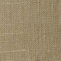
2       Wenbin Li, Mario Fritz

While grabbing large databases from the internet has been a promising direc-
tion pursued in recent years, it often comes with a bias and is less appropriate
for domains for which there is an underlying parametric structure that should
be learnt. Therefore we have seen increased interest in approaches that render
training data from 3D models. Probably one of the biggest success stories in this
field is the body pose estimation model from the Kinect that strongly leveraged
rendered depth maps for generating millions of training examples [1].
    However we realize that most successful applications of this data acquisi-
tion paradigm rely on 2D and/or 3D shape information and applications to
appearance-based descriptions has been limited. One possible explanation is that
despite rendering engines have become more and more powerful and appealing
to the human eye, the generated statistics are still different to real-world images.
The focus on features and application domains that rely on shape information
mask the problem that there is an underlying unsolved problem.
    Therefore we study in this paper the problem of appearance transfer from
rendered materials to real ones. In contrast to object or scene recognition we
have to entirely rely on appearance descriptors. We investigate different method
of combining real and virtual examples and formulating the mismatch of the two
data sources as an alignment or domain adaptation problem. Our approach pro-
poses a roadmap to scalable acquisition of rich models of material appearances,
as a large library of material shaders are available from companies that supply
the computer graphics domain or even for free from hobbyist and enthusiast.

Contributions: We present the first study on leveraging rendered materials for
the recognition of real materials. We show recognition from virtual data only
as well as improved performance by combining virtual and real data. We ana-
lyze how well different appearance descriptors can cope with this domain shift.
Beyond this, we also investigate the applicability of recent metric learning and
domain adaptation method to this problem which is the first principled approach
to deal with the discrepancies between rendered and real data examples. Our
study is based on a new database of virtual materials called MPI-VIPS which
complements the existing material database KTH-TIPS. The new database is
available at http://www.d2.mpi-inf.mpg.de/mpi-vips

2   Related Work

There is a long tradition of analyzing the visual appearance of texture and de-
riving good representations for this task [2, 3]. While earlier studies often looked
at single material instances as facilitated by the Curet database [4] the focus
shifted more towards recognizing whole material classes [5, 6], e.g. based on the
KTH-TIPS database. In order to even further increase intra class variance, a
web-based material recognition challenges has recently proposed [7, 8]. While
previous investigation have looked at a pure appearance based recognition chal-
lenge, this new database images whole objects and therefore investigates the
question how material recognition can be performed in context.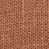
Recognizing Materials from Virtual Examples        3

    Recently, the generation of virtual training data has gained a lot of attention.
We distinguish two main threads: recombination and rendering. Recombination
methods leverage real examples and recombine aspects of them by certain model
assumption in order to form new ones. Examples include invariant support vec-
tor machines [9] that expand the support vector set by applying transformations
to them which are know to maintain class membership, generative pedestrian
models that can re-mix shape, appearance and backgrounds [10, 11].Also syn-
thesizing new views from real material samples has been investigated to expand
the training set [12]. On the other hand, rendering method generate genuinely
new examples from a model-based description. Probably the most prominent
approach is the recently presented approach to robust pose estimation from 3D
data that strongly leveraged rendered depth maps to attain the desired perfor-
mance [1]. A similar approach has been taken for object recognition in range
data by leveraging 3D model from google warehouse [13, 14]. Other applications
include 3D car models for learning edge-based shape representations of cars [15]
and scene matching from 3D city models [16] .
    As alluded to before, leveraging virtual training data tends to introduce some
discrepancy between the statistics of the real and the synthesized data. Distri-
bution mismatch between training and test time is a problem that relates to the
concept of domain shift. One of the first investigation in object recognition has
only been conducted quite recently [17, 18]. They employ metric learning [19] in
order to adapt data from the web to be more suitable for in situ recognition task.
Another example is the adaptation of rendered data to real examples [13] where
the domain adaptation approaches were used to adapt synthesized depth maps
from 3D google warehouse data for recognition in LIDAR scans. In contrast, this
paper conducts the first study on purely appearance-based descriptors for the
task of material recognition utilizing virtual examples.

3     Method

First, we describe our main recognition architecture and review the employed
feature descriptors. Then we explain the acquisition of virtual material exam-
ples and present the new database (MPI-VIPS) on which our study is based on.
Lastly, we describe the approaches we investigate in order to mitigate the discrep-
ancies between virtual data and real data. We propose an alignment procedures
tailored to the material recognition task. In addition we recap the “Frustratingly
Easy Domain Adaptation” approach [20] as well as a metric learning approach
[19] which we consider as generic machine learning approaches to this problem.

3.1   Material Recognition

Our main material recognition pipeline is based on a kernel classifier combined
with appearance features LBP and SIFT. Our choice of classifier and feature is
motivated by [5, 6, 8]. We continue with a brief review of the employed features
descriptors as well as the recognition architecture and choice of kernel.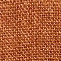
4      Wenbin Li, Mario Fritz

Multi-scale LBP The LBP descriptor [21] has shown to be a powerful description
of image texture. They key idea is to compute for each pixel a set of differences
to pixels in a local neighborhood. Depending on the sign of those differences, the
pixel is assigned a distinct pattern id. The final descriptor is a histogram of the
occurrences of such pattern id on an image patch of interest.
    The most prominent limitation of the LBP operator has been its small spa-
tial support area. Features calculated in a small local neighborhood cannot cap-
ture large-scale structures that may be the dominant features of some textures.
Several extensions have been introduced to overcome its limitations. We use
rotationally invariant, uniform LBP descriptor at 4 scales. Studies on the KTH-
TIPS2 database [5, 6] have shown strong performance for this descriptor on the
task of material classification.

Color Color is an important attribute of surfaces and can be a cue for mate-
rial recognition. Although color alone sometimes may be misleading, significant
boost have been reported (e.g. [8]) when combined with other descriptors. In
our experiment, we follow their scheme and extract color features from 5x5 pixel
patches.

Dense SIFT SIFT features have been widely used in scene and object recognition
to characterize the spatial and orientational distribution of local gradients and
it also has been shown to work well for material recognition task [8, 22]. In our
experiment, we again follow the setup of [8] and use dense SIFT.

Classification We use a Support-Vector-Machine (SVM) classifier. As previous
studies [6] and our own investigations have shown the described histogram-based
descriptors tend to show superior performance when used in combination with
an exponential-χ2 kernel [23]:

                           K(x, y) = exp{−αχ2 (x, y)}
                                       X |xi − yi |2
                           χ2 (x, y) =
                                       i
                                          |xi + yi |

Histograms were normalized to unit length and the kernel parameter α was found
by cross-validation on the training set.

3.2   Rendering
Bidirectional Reflection Functions (BRDF) give a full account on how light in-
teracts with a surface. Therefore they are a rich source to truthfully recreate the
appearance of material that carries discriminative information for classification
[24, 25]. This would make them the ideal source for synthesizing a virtual data
set.
    However their acquisition is tedious and time consuming – even more than the
generation of image datasets that we aim to circumvent. But the widespread use
of computer graphics rendering engines among professionals and hobbyists has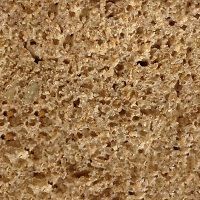
Recognizing Materials from Virtual Examples        5

lead to large libraries of material shaders that seek to capture the appearance of
materials in sufficient quality to yield photorealistic synthesis as well as provide
a computational efficient form to ensure fast rendering. 1000s of such material
shaders are available form commercial (e.g. DOSCH design) and free e.g. http:
//www.vray-materials.de) online sources. Being able to tab into those vast
resources would boost scalability of material recognition by up to two orders of
magnitude.
    Consequently, we propose to use approximative models as they are widely
used in the material shaders in most of the available rendering packages. In
particular we consider such material shaders that provide us with the following
3 informations:

Phong-type Shading Model We recollect that the basic Phong shading equations
is a combination of a ambient, a diffuse and a specular term. Therefore the light
intensity Lr (v̂r ; λ) observed in view direction v̂r at wavelength λ is given by:
                    Lr (v̂r ; λ) = ka (λ)La (λ) +
                                          X
                                   kd (λ)    Li (λ) < v̂i , n̂ >+ +
                                          i
                                          X
                                 ks (λ)       Li (λ)(< v̂r , ŝi >)ke
                                          i

where ka , kd , ks are the reflection distribution of the ambient, diffuse and spec-
ular part respectively (color of the object), La is the wavelength distribution of
the ambient illumination and Li is the wavelength distribution of the i-th light
source. The diffuse part is further governed by the angle between the surface
normal n̂ and the lighting direction v̂i of light source i and the specular part by
the angle between viewing direction and the specular reflection direction si . A
parameter ke controls the peakedness of the specular reflection.

Bump Map As 3D texture induced by the local micro structure of the material is
one very important effect which complicates robust classification [2], we require
our material shaders to provide a bump map. The method stores local variations
in geometry as a height map which is in turn used to compute a local normal.
This normal map is then used to modulates the original surface normal in order
to recreate shading effects of local 3D structure of the material.

Texture Map All our materials also come with a texture map that basically
encode the local and diffuse color of the material kd and also any other residual
effects. It is worth noting that for many material shaders available commercially
or online a visual appealing appearance is the prime modeling target and not
necessarily physical realism.

3.3   MPI-VIPS Database of rendered materials
We use the shader model described above to generate a new database of rendered
materials which we call MPI-VIPS (Virtual texture under varying Illumination,
6 Wenbin Li, Mario Fritz
Pose and Scales). One of our motivation is the availability of material shaders
from commercial suppliers to the computer graphics community as well as in-
ternet resources. We therefore collect a set of shaders that match the material
classes from the KTH-TIPS2 database in order to facilitate a systematic study.
To obtain the virtual data, we use Autodesk 3ds Max to do the rendering and
follow the scene setting in the KTH-TIPS2 database. In details, we vary the
distance from the rendered patch to camera to simulate the changes in scales
and apply directional light and ambient light to simulate the lighting condition
in the original database. Note all operations to change the scene settings can be
done precisely and easily with MAXScript in contrast to manually collection of
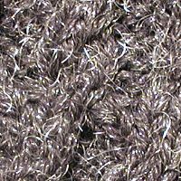
real world data. Fig 3 shows the rendered patches for the 11 material classes.
Next to them we also display the texture and bump maps included in the shader
information. While some of them show strong visual similarity to the true ma-
terials (e.g. bread (2nd row), cork (4th row), there are also significant variations
in style, color and detail. Several of the cloth samples show different color and
design patterns on them which make them very distinct from the examples in
the KTH-TIPS database. The same holds true for the level of realism. While
the above mentioned materials look quite realistic, examples with more com-
plex light interactions (e.g. aluminum foil (1st row), lettuce leaf (7th row)) look
artificial. We consider these properties to be an inherent characteristic of this
setting and consider this mix between good and bad matches as quite typical
and therefore well suited for our study.
3.4 Manifold Alignment
One concern when using rendered data is a mismatch in appearance when com-
pared to real examples. From a statistics point of view, we have one manifold
which is formed by the real examples and one which is formed by the rendered
ones. We would like to bring them to a coarse alignment by appropriate choice of
such rendering parameters. As we know the normal of the patch we are rendering
and we also use a rotation invariant descriptor, view point and rotation are less
concerning. However, we don’t get any notion of absolute scale from the shader
models. Therefore propose an alignment strategy that matches the scale of our
rendered examples to the real ones.
In details, there are 9 scales equally spaced logarithmically over two octaves,
3 different poses and 4 illumination conditions for each instance in the origi-
nal KTH-TIPS dataset. We choose a set of samples for each category with the
same pose, illumination conditions and placed at the 9 logarithmically equally
spaced scales{y1 , ..., y9 }, generate a series of N scales equally spaced logarith-
mically {x1 , x2 , ..., xN } as a pool of samples, and treat each consecutive 9 scales
starting from xi as one candidate alignment{xi , xi + 1, ..., xi + 8}. We com-
pute descriptor d on both samples and the candidates as {d(y1 ), ..., d(y9 )} and
{d(xi ), P
...d(xi + 8)}, then measure the accumulated difference between the two
n
sets as j=1 ∆(d(xi − 1 + j), d(yj )), where ∆ denotes for the difference between
the descriptors computed from Pn the two sets, can be either L1 and L2 distance.
We then choose i = argmin j=1 ∆(d(xi − 1 + j), d(yj )).
i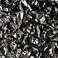
Recognizing Materials from Virtual Examples                                                                        7

                                                                    1.4
                                                                                                                                  aluminium foil
                                                                                                                                  brown bread
                                                                                                                                  corduroy
                                                                    1.2
                                                                                                                                  cork
                                                                                                                                  cotton
                                                                                                                                  cracker
                                                                     1                                                            lettuce leaf

                                             Accumulated Distance
                                                                                                                                  linen
                                                                                                                                  white bread
                                                                    0.8                                                           wood
                                                                                                                                  wool

                                                                    0.6

                                                                    0.4

                                                                    0.2

                                                                     0
                                                                          1   2   3   4    5     6   7     8   9   10   11   12
                                                                                          Starting Scale

Fig. 1. (Left) Illustration of our aligment approach. Nodes denote descriptors in differ-
ent scales, and lines with different colors denote different alignment of scales between
the baseline real samples and the candidate alignments. (Right) Coarse alignment with
scales. x-axis denotes different candidate scales and y-axis denotes accumulated differ-
ences between candidates and baseline samples.

    Figure 3.4 shows the resulting scores for different choices of alignment scales.
We see that most of the materials have a distinct minimum which – on visual
inspection – also corresponded to the correct scale. Two materials could not be
aligned with this procedure due to lack of a minimum. For those we had to pick
the scale manually. As we will show in our results, such an alignment step is
crucial for successfully utilizing rendered data.

3.5   Learning Approaches

While the previous section proposed a method of providing a first coarse align-
ment of the appearance manifolds, there are more subtle changes that differen-
tiate rendered and real examples. The challenge we face here is that we don’t
have a good handle how to parameterize those changes or even pin point the
exact discrepancies. Therefore we investigate metric learning and domain adap-
tation approaches that follow an exemplar-based paradigm. As we do have cor-
responding material patches in rough alignment, we can use them in such a
machine learning approach to learn a transformed space that is more robust to
the changes introduced by the two domains.

Metric Learning: Information theoretic metric learning (ITML) ITML [19] op-
timizes the Mahalanobis distance between each point pair xi , xj ∈ Rd

                         da (xi , xj ) = (xi − xj )T A(xi − xj )

It reduces to simple euclidean distance when A = I. To learn the metric matrix
A, the algorithm apply iterative procedures to minimizes the logdet divergence
between the current metric A and the initial matrix A0 with respect to pairwise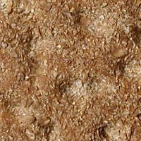
8       Wenbin Li, Mario Fritz

similarity constraints:
                      minimize       Dld (A, A0 )
                          A
                      subject to dA (xi , xj ) ≤ bu , (i, j) ∈ S
                                     dA (xi , xj ) ≥ bl , (i, j) ∈ D
where bu and bl are upper and lower bound of similarity and dissimilarity con-
straints. S and D are sets of similarity and dissimilarity constraints based on
the labeled data, namely pairs in the same categories are set with similarity
constraints, otherwise with dissimilarity constraints. The optimization is done
by repeated Bregman projections of a single constraint per iteration. It is also
convenient to extend the framework to a kernelized version that can also learn
non-linear deformations of the original space. In our experiment, we use the
kernel matrix instead of raw data and subsample 1 /4 of the full constraints to
reduce computational cost.

Frustratingly Easy Domain Adaptation Daume III [20] has introduced the “frus-
tratingly easy domain adaptation” by feature augmentation. In our experiment,
since we use exp −χ2 kernel for classification, we use a kernelized version of it.
For which, we define mapping
                              Φs = < Φ(x), Φ(x), 0 >                          (1)
                                 t
                              Φ = < Φ(x), 0, Φ(x) >                           (2)
where 0 =< 0, ..., 0 > is the zero vector, Φ(x) denotes the feature mapping in
the original space. This leads to the new kernel function:
                            2K(x, x0 ) if x,x0 are in the same domain

           K 0 (x, x0 ) =
                            K(x, x0 )  if x,x0 are in different domains

4     Experiments
In the experimental section we investigate how rendered materials can be utilized
to recognize real ones. Our investigation also evaluates methods that support the
transfer of appearance-based descriptors from the virtual to the real domain. We
report average accuracies over 4 trials by randomly splitting training and testing
data, while we always insure that we use different material instances in training
and test.

4.1   Datasets
We use two publicly available datasets in our experiments: the Flickr Material
Database and KTH-TIPS2 database. In addition we use our new database of
virtual materials MPI-VIPS (Virtual texture under varying Illumination, Pose
and Scale) which is intended to complement the KTH-TIPS (Texture under
varying Illumination, Pose and Scale) [5] database. Therefore it provides a test
bed for studying the transfer of appearance from rendered to real materials.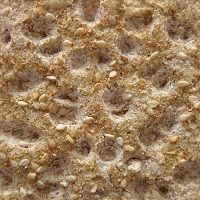
Recognizing Materials from Virtual Examples           9

                Method Feature          Classification Rate (%)
                aLDA Best Feature Comb.           44.6
                       SIFT                       35.2
                 Ours MLBP + Color                48.1
                       MLBP                       37.4

Table 1. Results. The classification rate with different sets of features for the Flickr
database.

The Flickr Material Database. The database is collected using Flickr photos
[7]. This includes 1000 images in 10 common material categories, ranging from
fabric, paper, and plastic, to wood, stone, and metal. State-of-the-art results
were obtained by exploring a large set of heterogeneous features and a Latent
Dirichlet Allocation (LDA) model [8]. We use this database in order to establish
reference for our recognition architecture to other recent approaches on material
recognition. Table 1 shows our results on the Flickr dataset and their combi-
nations. In our experiments on Flickr, we use kernelized SVM instead of aLDA
model but use the same experimental setting in order to stay comparable, and
we do four trials and report the average accuracies. The mlbp descriptor does
slightly better than any of the single features tested there (35%). By combing
color and mlbp, our test accuracy is 48.1% – higher than the reported one in
[8] (45%) and on par with most recent findings in [26] (48.2%). The competitive
performance shows the validity of our recognition approach for this task.
    We chose to not further study material recognition on this dataset as it con-
volutes the problem with object level biases. While we agree that this might be
intended in many applications, we want to restrict our study on pure appearance
aspects in the material recognition setting. Therefore the remaining part focuses
on the KTH TIPS database and its rendered counterpart MPI-VIPS.

KTH-TIPS2 Database The KTH-TIPS2 database [5] was designed to study
material recognition with a special focus on generalization to novel instances of
material. It includes 4608 images from 11 material categories, and each category
has 4 different instances. All the instances are imaged from varying viewing
angles (frontal, rotated 22.5◦ left and 22.5◦ ), lighting conditions (from the front,
from the side at 45◦ , from the top at 45◦ , and ambient light) and scales (9
scales equally spaced logarithmically over two octaves), which gives a total of
3 × 4 × 9 = 108 images per instance. We show examples of all the materials with
all their instances in Fig 3. Note the challenge posed by the intra-class variation
of the materials.
    The first block in Table 2 shows results of our recognition pipeline in the
standard setting. Each line represents a different of the 4 available material
instances into training and test. Our performance is on par with results shown
previously in this setup [5]. Best performance of 73.1% is obtained for 3 training
instances and Color+MLBP feature.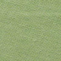
10      Wenbin Li, Mario Fritz

4.2   Can we recognize real materials from rendered examples?
The second and third block in Table 2 present our results training only on
rendered examples from the VIPS database and evaluating on the real examples
of the KTH TIPS database. The difference between the two is that the third
block is using the described manifold alignment procedure. We can see that the
alignment procedure increases the performance up to 11%. Overall, we observe
that the MLBP features seems to cope better with this domain shift than the
dense SIFT feature, leading to a performance of 43.7%. We hypothesize that the
binary feature are more reliable to extract than the gradient values in the SIFT
that might be easily effected by unrealistic reproduction of the materials. Adding
color information degrades performance in this setting which calls for another
alignment procedure to minimize those discrepancies between the domains which
we leave for future work.
    According the results, the conclusion must be that it is possible to recognize
real materials from rendered ones. However, we realize that there is still a signif-
icant performance gap between the information we get from a real instance and
a virtual one. The alignment step has proven critical to improve performance.

4.3   Mixing real and rendered examples
In the rest of the experimental section we ask the questions if there are ways to
combine real and rendered data in order to boost the performance. The 4th and
5th block of Table 2 show the results for a mixed training set of real and rendered
examples – again with and without the alignment procedure. While the results
without alignment either stay the same compared to training without rendered
data or even decrease, we observe up to 7% improvement after alignment. The
best performance of 80.2% is obtained for training on 1 rendered example and
3 real ones using the Color+MLBP.

4.4   Metric Learning
We also apply metric learning in an attempt to further bridge the gap between
the virtual and real materials. Therefore we build on top aligned data. Similarity
constraints are generated between the virtual and real materials of the same class
and also dissimilarity constraints between different materials. The results are
presented in the 6th block of Table 2. Again, the dense SIFT descriptor performs
consistently worse and the metric learning doesn’t provide improvements. On
the other descriptors, we do see a small improvement when only one or two real
materials are observed at training time.

4.5   Domain Adaptation
Lastly, we apply the “frustratingly easy” domain adaptation technique to this
problem. The last block in Table 2 shows the results. The previous result is kind
of reversed. While this method shows marginally increased performance for the
dense SIFT descriptor when only one or two examples are available, no effect
can be observed for the other two features.
Recognizing Materials from Virtual Examples 11
4.6 Discussion
Concerning the detailed changes brought by the virtual data and different de-
scriptor, there were some interesting observations: when introducing color fea-
tures, we experienced a slight performance decrease for corduroy - which can
be explained by the different coloration in the virtual materials; there was good
improvement with rendered material in general, but on some particular more
complex materials(e.g. aluminum foil) the performance degraded.
5 Conclusions
We have presented a new database MPI-VIPS of rendered materials that allows
to study the challenges when learning the appearance of real materials from
or supported by rendered materials. We have shown the feasibility and present
results indicating that LBP based features are more suited to this task as SIFT
based representations. We further evaluate different approaches to deal with the
appearance mismatch ranging from mixed training sets, data alignment, metric
learning and domain adaptation. Our results suggest that an alignment of the
two data sources is crucial and in combination with a kernel classifier trained on
mixed real and rendered data we obtain a significant performance improvement
of 7%.
Acknowledgments. Wenbin Li was supported by the scholarship from the
Saarbrücken Graduate School of Computer Science, Saarland University.
References
1. Shotton, J., Fitzgibbon, A., Cook, M., Sharp, T., Finocchio, M., Moore, R., Kip-
manand, A., Blake, A.: Real-time human pose recognition in parts from a single
depth image. In: CVPR. (2011)
2. Leung, T., Malik, J.: Representing and recognizing the visual appearance of ma-
terials using three-dimensional textons. IJCV (2001)
3. Varma, M., Zisserman, A.: A statistical approach to texture classification from
single images. IJCV (2005)
4. Dana, K., van Ginneken, B.: Reflectance and texture of real-world surfaces. In:
CVPR. (1997)
5. Hayman, E., Caputo, B., Fritz, M., Eklundh, J.O.: On the significance of real-world
conditions for material classification. In: ECCV. (2004)
6. Caputo, B., Hayman, E., Mallikarjuna, P.: Class-specific material categorisation.
In: ICCV. (2005)
7. Sharan, L., Rosenholtz, R., Adelson, E.H.: Material perception: What can you see
in a brief glance? Journal of Vision (2009)
8. Liu, C., Sharan, L., Adelson, E.H., Rosenholtz, R.: Exploring features in a bayesian
framework for material recognition. In: CVPR. (2010)
9. Decoste, D., Schölkopf, B.: Training invariant support vector machines. Mach.
Learn. 46 (2002) 161–19012 Wenbin Li, Mario Fritz
10. Enzweiler, M., Gavrila, D.M.: A mixed generative-discriminative framework for
pedestrian classification. In: CVPR. (2008)
11. Pishchulin, L., Jain, A., Wojek, C., Andriluka, M., Thormaehlen, T., Schiele, B.:
Learning people detection models from few training samples. In: CVPR. (2011)
12. Targhi, A.T., Geusebroek, J.M., Zisserman, A.: Texture classification with minimal
training images. In: IEEE International Conference on Pattern Recognition. (2008)
13. Lai, K., Fox, D.: 3D laser scan classification using web data and domain adaptation.
In: Proceedings of Robotics: Science and Systems. (2009)
14. Wohlkinger, W., Vincze, M.: 3d object classification for mobile robots in home-
environments using web-data. In: International Conference on Cognitive Systems
(CogSys). (2010)
15. Stark, M., Goesele, M., Schiele, B.: Back to the future: Learning shape models
from 3d cad data. In: BMVC. (2010)
16. Kaneva, B., Torralba, A., Freeman, W.: Evaluation of image features using a
photorealistic virtual world. In: ICCV. (2011)
17. Saenko, K., Kulis, B., Fritz, M., Darrell, T.: Adapting visual category models to
new domains. In: ECCV. (2010)
18. Kulis, B., Saenko, K., Darrell, T.: What you saw is not what you get: Domain
adaptation using asymmetric kernel transforms. In: CVPR. (2011)
19. Davis, J., Kulis, B., Jain, P., Sra, S., Dhillon, I.: Information-theoretic metric
learning. In: ICML. (2007)
20. Daumé III, H.: Frustratingly easy domain adaptation. In: Conference of the
Association for Computational Linguistics (ACL). (2007)
21. Ojala, T., Pietikäinen, M., Harwood, D.: A comparative study of texture measures
with classification based on featured distributions. Pattern Recognition (1996)
22. Zhang, J., Marszalek, M., Lazebnik, S., Schmid, C.: Local features and kernels for
classification of texture and object categories: a comprehensive study. IJCV (2007)
23. Chapelle, O., Haffner, P., Vapnik, V.: Svms for histogram-based image classifica-
tion. In: IEEE Transactions on Neural Networks. (1999)
24. Nillius, P., Eklundh, J.O.: Classifying materials from their reflectance properties.
In: ECCV. (2004)
25. Wang, O., Gunawardane, P., Scher, S., Davis, J.: Material classification using brdf
slices. In: CVPR. (2009)
26. Liu, L., Fieguth, P., Kuang, G., Zha, H.: Sorted random projections for robust
texture classification. In: ICCV. (2011)Recognizing Materials from Virtual Examples 13
train on real – test on real
Setting Dense SIFT MLBP Color+MLBP
1 real train + 3 real test 45.5(±3.6) 59.1(±3.7) 61.4(±2.8)
2 real train + 2 real test 52.3(±2.3) 65.8(±1.4) 70.4(±0.7)
3 real train + 1 real test 56.4(±2.6) 70.7(±3.2) 73.1(±4.6)
train on unaligned virtual – test on real
Setting Dense SIFT MLBP Color+MLBP
1 virtuall train + 3 real test 26.7(±1.2) 31.9(±1.6) 31.3(±2.5)
train on aligned virtual – test on real
Setting Dense SIFT MLBP Color+MLBP
1 virtual train + 3 real test 33.1(±1.2) 43.7(±2.1) 40.3(±2.7)
train on mix of unaligned virtual and real – test on real (kernel-SVM)
Setting Dense SIFT MLBP Color+MLBP
1 virtual train + 1 real train + 3 real test 42.4(±1.8) 59.3(±4.0) 59.9(±1.8)
1 virtual train + 2 real train + 2 real test 53.6(±1.3) 67.1(±2.5) 66.8(±3.4)
1 virtual train + 3 real train + 1 real test 52.4(±1.1) 70.0(±1.4) 73.2(±4.7)
train on mix of aligned virtual and real – test on real (kernel-SVM)
Setting Dense SIFT MLBP Color+MLBP
1 virtual train + 1 real train + 3 real test 45.1(±2.3) 62.2(±2.7) 63.8(±1.4)
1 virtual train + 2 real train + 2 real test 51.8(±2.5) 69.2(±1.2) 68.2(±1.8)
1 virtual train + 3 real train + 1 real test 54.4(±2.9) 72.5(±4.1) 80.2(±4.5)
train on mix of aligned virtual and real – test on real (metric learning)
Setting DenseSift MLBP Color+MLBP
1 virtual train + 1 real train + 3 real test 43.2(±2.3) 62.4(±4.0) 64.1(±2.0)
1 virtual train + 2 real train + 2 real test 46.7(±2.5) 65.7(±1.3) 68.7(±2.6)
1 virtual train + 3 real train + 1 real test 50.9(±2.9) 71.8(±1.5) 74.7(±2.4)
train on mix of aligned virtual and real – test on real (FE domain adaption)
Setting Dense SIFT MLBP Color+MLBP
1 virtual train + 1 real train + 3 real test 47.8(±2.5) 59.3(±3.7) 59.8(±1.3)
1 virtual train + 2 real train + 2 real test 52.8(±2.4) 66.1(±1.9) 65.3(±1.0)
1 virtual train + 3 real train + 1 real test 55.2(±2.4) 70.9(±3.2) 72.8(±2.5)
Table 2. Results on KTH TIPS and the new VIPS database14 Wenbin Li, Mario Fritz
New VIPS database of virtual materials KTH-TIPS material database
texture bump map rendered sample real samples
Table 3. Example images of the new material database (VIPS) of rendered examples
from material shaders on the left and corresponding examples from the KTH TIPS
database on the right. Please note that these are only the canonical view points and
both databases incorporate variations in scale, viewpoint and lighting.You can also read