WASP: Scalable Bayes via barycenters of subset posteriors
←
→
Page content transcription
If your browser does not render page correctly, please read the page content below
WASP: Scalable Bayes via barycenters of subset posteriors

Sanvesh Srivastava1,2          Volkan Cevher3              Quoc Tran-Dinh3           David B. Dunson1
ss602@stat.duke.edu         volkan.cevher@epfl.ch       quoc.trandinh@epfl.ch          dunson@duke.edu
             Department of Statistical Science, Duke University, Durham, North Carolina, USA1
     Statistical and Applied Mathematical Sciences Institute (SAMSI), Durham, North Carolina, USA2
 Laboratory for Information and Inference Systems, École Polytechnique Fédérale de Lausanne, Switzerland3

                      Abstract                                subset-specific optimization problems. One widely
                                                              used and well understood framework is ADMM [4; 6].
                                                              In Bayesian statistics, one is faced with the more chal-
    The promise of Bayesian methods for big
                                                              lenging problem of approximating a posterior measure
    data sets has not fully been realized due
                                                              for the unknown parameters instead of just obtaining
    to the lack of scalable computational algo-
                                                              a single point estimate of these parameters. Poste-
    rithms. For massive data, it is necessary to
                                                              rior measures have the major advantage of providing
    store and process subsets on different ma-
                                                              a characterization of uncertainty in parameter learn-
    chines in a distributed manner. We propose
                                                              ing and predictions; such uncertainty quantification
    a simple, general, and highly efficient ap-
                                                              is lacking for many optimization approaches. How-
    proach, which first runs a posterior sampling
                                                              ever, a fundamental disadvantage is the lack of scalable
    algorithm in parallel on different machines for
                                                              computational algorithms for accurately approximat-
    subsets of a large data set. To combine these
                                                              ing posterior measures in general Bayesian models.
    subset posteriors, we calculate the Wasser-
    stein barycenter via a highly efficient lin-              The main workhorse of Bayesian posterior computa-
    ear program. The resulting estimate for the               tion is Markov chain Monte Carlo (MCMC) sampling,
    Wasserstein posterior (WASP) has an atomic                with variants such as sequential Monte Carlo (SMC)
    form, facilitating straightforward estimation             and adaptive Monte Carlo being also popular. Such
    of posterior summaries of functionals of in-              Monte Carlo algorithms obtain samples from the pos-
    terest. The WASP approach allows posterior                terior measure, which are used to estimate summaries
    sampling algorithms for smaller data sets to              of the posterior and predictive distributions of interest.
    be trivially scaled to huge data. We provide              These algorithms for posterior sampling are applicable
    theoretical justification in terms of posterior           to essentially any Bayesian model, but face computa-
    consistency and algorithm efficiency. Exam-               tional bottlenecks in scaling up to large data sets. Such
    ples are provided in complex settings includ-             bottlenecks can potentially be addressed by using data
    ing Gaussian process regression and nonpara-              subsets to define subset posterior measures, which pro-
    metric Bayes mixture models.                              vide a noisy approximation to the posterior measure
                                                              based on the full data. After applying Monte Carlo al-
                                                              gorithms to obtain samples from each subset posterior
1    Introduction                                             in parallel, the goal is then to efficiently combine these
                                                              samples to obtain samples from an approximation to
Efficient computation for massive data commonly re-           the posterior measure for the full data.
lies on using small subsets of the data in parallel, com-     This article focuses on fundamentally improving the
bining results of local computations to obtain global         combining step, bypassing the need to introduce a
results. The usual focus is on obtaining parame-              kernel or tuning parameters, while massively speed-
ter estimates, which minimize a loss function based           ing up computations. In particular, the proposed ap-
on the complete data, by dividing computation into            proach combines samples from subset posterior mea-
                                                              sures by calculating the barycenter with respect to a
Appearing in Proceedings of the 18th International Con-       Wasserstein distance between measures. The resulting
ference on Artificial Intelligence and Statistics (AISTATS)   Wasserstein posterior (WASP) can be estimated effi-
2015, San Diego, CA, USA. JMLR: W&CP volume 38.
Copyright 2015 by the authors.                                ciently via a linear program, and has an atomic form,
WASP: Scalable Bayes via barycenters of subset posteriors
making calculation of posterior and predictive sum- a kernel and corresponding bandwidth. The resulting
maries trivial. The WASP framework is tuned for dis- median posterior provides a robust alternative to the
tributed computations. Posterior samples from local true posterior. Inspired by this idea, we focus on ap-
computations are combined in the final step to yield a proximating the true posterior instead of robustifying
posterior distribution that is close to the true posterior it. This removes the need for the RKHS embedding
distribution with respect to a Wasserstein distance. and vastly speeds up the computation time. Extend-
ing the Sinkhorn algorithm of Cuturi [8], Cuturi and
Current scalable Bayes methods belong to three ma-
Doucet [9] estimate the WB of empirical measures us-
jor groups. The first group estimates an approximate
ing entropy-smoothed subgradient methods. We in-
posterior distribution that is closest to the true poste-
stead estimate the WASP by solving a LP and effi-
rior while restricting the search to a parametric family.
ciently obtain its solution by exploiting the sparsity of
While these methods have restrictive distributional as-
LP constraints.
sumptions, they can be made computationally efficient
[24; 3; 5; 15; 14; 19]. The second group exploits the
analytic form of posterior and uses computer architec- 2 Preliminaries
ture to improve the sampling time and convergence
[20; 22; 1]. This approach is ideal for large-scale ap- We first describe the Wasserstein space of probabil-
plications that use simple parametric models. The ity distributions, with the Wasserstein distance as
third group obtains subset posteriors using some sam- a natural metric. We then recall the relation be-
pling algorithm and combines them by using kernel tween Wasserstein distance and the objective of op-
density estimation [18], Weierstrass transform [23], or timal transportation problems. Based on these ideas,
minimizing a loss defined on the reproducing kernel we highlight the role of the WB as a summary of a col-
Hilbert space (RKHS) embedding of the subset poste- lection of posterior distributions for scalable Bayesian
riors [16]. These methods are flexible in that they are inference.
not restricted to a parametric class of models; how-
ever, the results can vary significantly depending on 2.1 Notations
the choice of kernels without a principled approach for
kernel choice. The ordered pair (Θ, d) represents a metric space
Θ with metric d. In this work, we are only con-
The WASP framework relies on two general assump- cerned with complete separable metric space (Pol-
tions that are frequently satisfied in Bayesian applica- ish space). The space of Borel probability measures
tions. These assumptions relate the parameter space on Θ is represented by P(Θ). The symbol δθ0 de-
and the associated space of probability measures: notes the Dirac measure concentrated at θ 0 ∈ Θ, i.e.,
δθ0 (A) = 1{θ 0 ∈ A} for any Borel measurable set A.
(a) The parameter space is a metric space.
If ψ is a Borel map Θ → Θ and ν is a measure on Θ,
(b) The atomic approximations of the subset poste- then the push-forward
R of ν through ψR is the measure
riors (empirical measures) can be obtained effi- ψ#ν defined as Θ f (y)d(ψ#ν)(y) = Θ f (ψ(x))dν(x)
ciently using a posterior sampler. for every continuous bounded function f on Θ. The N -
dimensional simplex is ∆N = {a ∈ RN |∀n ≤ N, 0 ≤
PN
Assumption (a) is frequently satisfied in practice us- an ≤ 1, n=1 an = 1} and Θ(n) represents the n-
ing the Euclidean distance. Assumption (b) can be dimensional Cartesian product Θ × . . . × Θ. We repre-
typically satisfied if the subset size and the number of sent the Frobenius inner product between two matrices
unknown parameters are not too large. Due to the ge- A and B as hA, Bi = tr(AT B) and k · k2 denotes the
ometric properties of the Wasserstein metric [21], the standard Euclidean distance.
Wasserstein barycenter (WB) of the subset posteri-
ors has highly appealing statistical and computational 2.2 Wasserstein space and distance
properties. We formulate a linear program (LP) to es-
timate the (atomic) WB of atomic approximations of The Wasserstein space of order p ∈ [1, ∞) of proba-
subset posteriors. Exploiting the sparsity of the LP, bility measures on (Θ, d) for an arbitrary θ 0 ∈ Θ is
we efficiently estimate the WB using standard soft- defined as
ware, such as Gurobi [13]. Z
p
The WASP framework is inspired from recent develop- P p (Θ) := µ ∈ P(Θ) : d(θ 0 , θ) dµ(θ) < ∞ ,
Θ
ments in optimal transport problems [8; 9] and scalable (1)
Bayes methods [16]. Minsker et al. [16] proposed to
use the geometric median of subset posteriors, calcu- and P p (Θ) is independent of the choice of θ 0 . The
lated using a RKHS embedding that required choice of Wasserstein distance of order p between µ, ν ∈ P(Θ)Srivastava, Cevher, Tran-Dinh, and Dunson
is defined as where the last equality is implied by the definition of
Z 1/p W2 (2); see [8] for details. The worst case complexity
Wp (µ, ν) := inf d(θ 1 , θ 2 )p dτ (θ 1 , θ 2 ) , of solving (5) scales as O((N1 N2 )3 log(N1 N2 )). Moti-
τ ∈T (µ,ν) Θ(2) vated by this limitation, Cuturi [8] smoothed the ob-
(2) jective in (5) using entropy and derived an efficient al-
gorithm for calculating optimal T based on Sinkhorn
where T (µ, ν) is the set of all probability measures on algorithm. This approach, however, has limited appli-
Θ(2) with marginals µ and ν, respectively. Wp is at- cations since the parameter that controls the amount
tractive in that it metrizes the weak convergence on Θ of entropy-smoothing needs to be specified apriori, and
and preserves the geometry of the space. An impor- the results can be sensitive to its choice.
tant topological property of P p (Θ) that will used later
in proving posterior consistency is as follows.
2.4 Wasserstein barycenter
Theorem 2.1 ([21]) If (Θ, d) is a Polish space and
p ∈ [1, ∞), then (P p (Θ), Wp ) is a Polish space. More
specifically,
(a) Given > 0, an arbitrary θ 0 in a dense subset
of Θ, and µ ∈ P 2 (Θ), there exists a compact set
Θ ⊂ Θ such that Θ \ Θ d(θ 0 , θ)p dµ(θ) < p .
R
(b) ∃M < ∞ such that k θ k < M ∀ θ ∈ Θ .
We focus on Θ ⊂ RD , d = k · k2 , and metric space
(P 2 (Θ), W2 ).
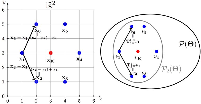
Figure 1: Barycenter in R2 and P 2 (Θ). The Euclidean
2.3 Wasserstein distance as a solution of an and Wasserstein barycenters are represented as xK
optimal transport problem and ν K (in red) when K = 6 and λk = 1/6 in (6) and
(7). The arrows represent constant speed geodesics in
If µ and ν are discrete probability measures, then R2 and P 2 (Θ), respectively. The geodesic in R2 is the
W2 (µ, ν) (2) is the minimum objective function value straight line joining two points, where as the geodesic
of a discrete optimal transport problem [8]. Let µ in P 2 (Θ) corresponds to the measure preserving map
N1 ×D T1j such that νj = T1j #ν1 for j = 2, 6.
PN1 on Θ1 ∈ R
and ν be atomic measures supported
N2 ×D
and Θ2 ∈ R so that µ = n=1 an δθT1 and that
n
ν =
PN2
, where a ∈ ∆N1 , b ∈ ∆N2 , and WB generalizes the Euclidean barycenter (EB) to
n=1 bn δθ T
2 n P 2 (Θ). If x1 , . . . , xK ≡ x1:K ∈ RD , then their EB
θ Tin is the n-th row of Θi . The discrete optimal trans- PK
xK,λ = k=1 λk xk for λ ∈ ∆K is such that
port problem is formulated in terms of (a) the matrix
1 ×N2
M12 ∈ RN + of pairwise squared distances between K K
the collection of atoms in Θ1 and Θ2 ; and (b) the op-
X X
λk k xk −xK,λ k22 = inf λk k xk − y k22 ; (6)
timal transport polytope that is the set of all feasible y∈RD
k=1 k=1
solutions called transport plans. The (i, j)-th entry of
M12 is see Figure 1. Generalizing (6) to P 2 (Θ), Agueh and
Carlier [2] showed that if ν1 , . . . , νK ≡ ν1:K ∈ P 2 (Θ),
[M12 ]ij = k θ 1i − θ 2j k22 . (3) then their WB ν K,λ for λ ∈ ∆K is such that
The optimal transport polytope is defined as K K
X X
1 ×N2 λk W22 (νk , ν K,λ ) = inf λk W22 (νk , ν); (7)
T (a, b) = {T ∈ RN
+ : T 1N2 = a, TT 1N1 = b}; ν∈P 2 (Θ)
k=1 k=1
(4)
see Figure 1. Agueh and Carlier [2] also showed that
therefore, transport plan T ∈ T (a, b) is a N1 × N2
ν K,λ in (7) can be obtained as a solution to a LP prob-
doubly stochastic matrix such that its row sums equal
lem posed as a multimarginal optimal transportation
a and its column sums equal b. Based on (3) and (4),
problem [11]. We only present their main result that
the objective of discrete optimal transport problem is
relates ν K,λ and ν1:K . Recall that if σ is a Borel map
dM12 (a, b) := min hT, M12 i = W22 (µ, ν), (5) RD → RD , then the push-forward of µ through σ is
T∈T (a,b) the measure σ#µ; see Section 2.1. If T1k representsWASP: Scalable Bayes via barycenters of subset posteriors
(n)
the measure preserving map from ν1 to νk such that Pθ0 = Pθ∞0 (X (n) )−1 for all n and θ 0 ∈ Θ is unknown.
νk = T1k #ν1 for k = 1, . . . , K, then Given a Bayesian model, we obtain the (random) pos-
! terior distribution Πn (·|X (n) ). A version of Bayes the-
K
X
1 orem implies that for all Borel measurable U ⊂ Θ
ν K,λ := λk Tk #ν1 (8)
R Qn
k=1 p(Xi | θ)d Πn (θ)
Πn (U |X ) = RU Qi=1
(n)
n . (9)
generalizes the EB (6) to WB (7) in P 2 (Θ) [2]. We Θ i=1 p(Xi | θ)d Πn (θ)
use this result later in proving Theorem 3.3; see The-
orem 4.1 and Proposition 4.2 of [2] for greater details. The following is a useful notion of consistency that
We also note that there are many formulations of (7) characterizes the behavior of random posterior distri-
in literature but have been solved using different tools bution Πn (U |X (n) ) as n → ∞.
or appear under different names [9]. Extending the
Definition 3.1 (Strong Consistency) A posterior dis-
Sinkhorn algorithm [8], Cuturi and Doucet [9] propose
tribution Πn (·|X (n) ) is said to be strongly consistent at
two fast algorithms for calculating entropy-smoothed
θ 0 if Πn (·|X (n) ) →w δθ0 as n → ∞ a.s. [Pθ∞0 ].
versions of ν K,λ using gradient based methods. The
WASP framework reformulates (7) as a sparse LP This is a stronger notion of consistency in that strong
problem that is computationally efficient without re- consistency of Πn (·|X (n) ) implies that there exists a
quiring any entropy-smoothing. consistent estimator of θ 0 . It is well-known that under
fairly general conditions Πn (·|X (n) ) is strongly consis-
3 Contributions and main results tent at θ 0 [12]. A necessary condition for posterior
consistency to hold states that the prior must assign
This section proposes to combine a collection of sub- positive probabilities to every Kullback-Leibler (KL)
set posteriors using their WB called WASP. We prove neighborhood of θ 0 .
that WASP is strongly consistent at the true value
θ 0 ∈ Θ. Specifically, WASP converges weakly to δθ0 Definition 3.2 (KL property) Let θ ∼ Π. Then Π
in (P 2 (Θ), W2 ). We also modify the subset posteriors has KL property at θ 0 ∈ Θ, if Π(K (θ 0 )) > 0 ∀ > 0,
appropriately so that the uncertainty quantification of where K (θ 0 ) = {θ : KL(pθ0 ||qθ ) < }, for densities
the WASP is well-calibrated. Finally, we reformulate pθ0 and qθ with
R respect to the reference measure ν, and
(7) as a sparse LP for fast estimation of WASP. KL(f ||g) = f log fg dν. This property is represented
as θ 0 ∈ KL(Π).
3.1 Wasserstein Barycenter for scalable
Intuitively, the KL property requires the prior to as-
Bayesian inference
sign positive probability to any small neighborhood of
We first highlight important topological properties of θ 0 . If this property is not satisfied, then it is well-
the metric space (Θ, k·k2 ) that will be used for proving known that the posterior Πn (·|X (n) ) might fail to con-
theoretical properties of the WASP. Let {Pθ : θ ∈ Θ} centrate around θ 0 even when n → ∞.
be a family of probability distributions parameterized Posterior sampling for massive data is frequently in-
by Θ ⊂ RD . The norm topology of (RD , k · k2 ) when tractable in Bayesian applications. A typical divide-
restricted to Θ implies that (Θ, k · k2 ) is also a Polish and-conquer strategy randomly partitions X (n) into K
space. Using Theorem 2.1, W2 metrizes the topology subsets X[k] and obtains subset posteriors Πkn (·|X[k] )
of weak convergence in P 2 (Θ). For all θ ∈ Θ, Pθ is for k = 1, . . . , K. Without loss of generality, we as-
assumed to be absolutely continuous with respect to sume that each subset is of size m so that n = Km.
the Lebesgue measure dx on RD so that dP (·| θ) = The following lemma is used to prove strong consis-
p(·| θ)dx. All statements regarding the convergence of tency of subset posteriors. It is similar in spirit to
measures in the context of WASP are in the metric Theorem 2.1 of Ghosal et al. [12]. All proofs are in-
space (P 2 (Θ), W2 ). cluded in the supplementary materials.
We now recall some basic concepts from nonparametric
Bayes theory. Most of these concepts and definitions Lemma 3.1 Let Θ be a compact subset of RD , let
are based on fundamental results of [12]. Let C be P 2 (Θ) be the Wasserstein space of probability mea-
the Borel σ-field on Θ and Πn be a (prior) probability sures parametrized by θ ∈ Θ, and let the true measure
measure on (Θ, C). Suppose that we observe random δθ0 ∈ P 2 (Θ). Given > 0, Θ is a compact subset of
variables (X1 , . . . , Xn ) ≡ X (n) that are independent Θ that satisfies (a) in Theorem 2.1, M is a large num-
and identically distributed as Pθ0 for some unknown ber that satisfies (b) in Theorem 2.1, and Πn satisfies
θ 0 ∈ Θ. Assume that random variables X (n) are de- the KL property ∀n such that liminf Πn (K (θ 0 )) > 0
n→∞
fined on the fixed measurable space (Ω, A) and that ∀ > 0. Then, Πn (·|X (n) ) is strongly consistent at θ 0 .Srivastava, Cevher, Tran-Dinh, and Dunson
Intuitively, Lemma 3.1 states that the posterior mea- preserving map T1k for k = 1, . . . , K. The following
sure Πn (·|X (n) ) assigns probability 1 to any neigh- theorem states the main results of this subsection that
borhood of θ 0 as n → ∞ if conditions (a) and (b) Πn (11) is strongly consistent at θ 0
of Theorem 2.1 and the KL property hold. Fur-
thermore, if m → ∞, then the following proposition Theorem 3.3 If all the conditions of Lemma 3.1
proves that Πkn (·|X[k] ) are strongly consistent at θ 0 hold, then Πn (11) is strongly consistent at θ 0 .
for k = 1, . . . , K as a straightforward application of
Intuitively, this theorem states that the mean of noisy
Lemma 3.1.
approximations of the true posterior in P 2 (Θ) is also
Proposition 3.1 Under the conditions of Lemma a good approximation of the true posterior.
3.1, if m → ∞, then subset posteriors Πkn (·|X[k] ) for Theorem 3.3 can be improved substantially to yield
k = 1, . . . , K are strongly consistent at θ 0 . rate of contraction using the construction of sieves in-
1
troduced by [12]. Given a decreasing sequence (n )n∈N ,
It is clear that the subset posteriors use only K frac- prior sequence (Πn )n∈N ∈ P 2 (Θ), and universal con-
tion of the whole data, so the credible intervals ob- stants B, b > 0, there exists sequence of increasing
tained from Πkn s will be wider than the credible in- compact parameter spaces Θn ⊂ Θ and polynomially
terval obtained from a posterior distribution that uses increasing sequence (Mn )n∈N such that
the whole data; that is, subset posteriors over-estimate
the uncertainty in the unknown parameters. Minsker (A1) Πn (Θcn ) ≤ B exp(−bn) (“tight prior ”);
et al. [16] addressed this issue by using a “stochastic
approximation (SA) trick.” This idea compensates for (A2) Mn2 exp(−nb) → 0 as n → ∞ (“polynomially in-
the data lost due to partitioning by adding (K − 1) creasing Mn s” );
extra copies of X[k] in each subset for k = 1, . . . , K.
(A3) Θn = {θ ∈ Θ : k θ k2 ≤ Mn } (“polynomially
The resulting subset posteriors are noisy estimates of
bounded parameter space”);
the full data posterior, and do not vary systematically
from the overall posterior in mean, variance, or shape. (A4) the packing number satisfies log N (n , Θn , k.k2 ) ≤
WASP also uses the SA trick for each of the subset n2n .
posteriors, obtaining subset posteriors that are dis-
tributed randomly around the overall posterior. The Then, the following theorem states that under assump-
subset posteriors using SA trick are defined as tions (A1) - (A4), Πn (·|X1:n ) is strongly consistent at
R Qm K θ 0 if the prior satisfies the KL property.
p(X[k]i | θ) d Πn (θ)
ΠSA
kn (U | X[k] , . . . , X[k] ) = R U i=1
.
| {z }
Qm
p(X[k]i | θ)
K
d Πn (θ) Theorem 3.4 Let Θ be compact subset of RD , let
Θ i=1
K
P 2 (Θ) be the Wasserstein space of probability measures
(10)
parametrized by θ ∈ Θ, and let the true measure δθ0 ∈
for k = 1, . . . , K and Borel measurable U ⊂ Θ. The P 2 (Θ). Assume that the sequences (Θn )n∈N ⊂ Θ and
next proposition states that SA-corrected subset pos- (Mn )n∈N satisfy Assumptions (A1) – (A3) for univer-
teriors are also strongly consistent at θ 0 . sal constants B, b and sequences (n )n∈N , (Πn )n∈N ∈
P 2 (Θ) and that Πn satisfies the KL property ∀n such
Proposition 3.2 Under the conditions of Lemma that liminf Πn (K (θ 0 )) > 0 ∀ > 0. Then, Πn (·|X1:n )
n→∞
3.1, the subset posteriors with stochastic approxima- is strongly consistent at θ 0 .
tion ΠSA
kn (·|X[k] ) for k = 1, . . . , K are strongly consis-
tent at θ 0 . Further, it follows from Theoremq3.4 of [16] and [12,
Section 5] that if we choose n ' K log
n
n
and we take
This lemma is follows from Lemma 3.1 by noticing that
K = O(log n) in Theorem 3.4, then we differ from the
m → ∞ =⇒ Km → ∞.
optimal rate of n−1/2 by a factor of only log n.
SA
The WASP Πn is the WB ΠK,λ for a given λ ∈ ∆K
and SA-corrected subset posteriors ΠSA1n :Kn (7). Fol- 3.2 Wasserstein barycenter of empirical
lowing (8), Πn has the following analytic form probability measures based on LP
K
! The analytic form of Πn (11) is tractable but for most
SA X
Πn (·|X (n)
) := ΠK,λ = λk T1k # ΠSA
1n , (11) practical problems the maps T1k s are analytically in-
k=1 tractable. One solution is to estimate Πn from pos-
terior samples of ΠSA
kn s. Several simulation-based ap-
1
where ΠSA SA
kn = Tk # Π1n is the push-forward of SA- proaches, such as MCMC, SMC, and importance sam-
corrected subset posterior ΠSA
1n through the measure pling, can be used to generate samples from ΠSA kn s forWASP: Scalable Bayes via barycenters of subset posteriors
a large class of models. In this work, we focus on the where T (a, bk ) is defined in (4). The optimal trans-
special case when the reference measure is a uniform port plan between a and bk , T b k (a), is obtained as
distribution on a finite collection of atoms in Θ.
b k (a) = argmin hTk , Mk i
T (16)
We assume that the subset posteriors are empirical Tk ∈T (a,bk )
measures and their atoms are simulated from the sub-
set posteriors using a sampler. Let Θ e ∈ RN ×D be for k = 1, . . . , K. To account for unknown a, an exten-
a collection of N such posterior samples ∈ Θ. If θeT sion of (16) based on (5) and (7) under the assumption
n
represents the n-th row of Θ,
e then the empirical prob- that λk = 1/K yields
ability measure corresponding to Θ
e is defined as K
X
N T
b 1, . . . , T
bK, a
b= argmin hTk , Mk i .
X 1 T1 ,...,TK ,a,
πN = δθeT . (12) a∈∆N ,
k=1
n=1
N n
Tk ∈T (a,bk ) k=1,...,K
(17)
Empirical measures are routinely used to approximate
posterior measures; however, for the approximation of If we represent
the joint measure to be accurate, the number of atoms
K
N must be very large. The WASP combines ΠSA kn k=1 ,
vec(M) = vec([M1 . . . , Mk , . . . , MK ]),
which are assumed to be empirical probability mea- vec(T) = vec([T1 . . . , Tk , . . . , TK ]),
sures, by estimating their barycenter Πn . The esti-
mation procedure is such that Πn is estimated as an and bT = (bT1 , . . . , bTk , . . . , bTK ), then (17) reduces to
empirical probability measure.
min vec(M)T vec(T) + 0TN ×1 a
We first set up the problem of WASP estimation in
vec(T)
a
form of (5). Following (12), assume that posterior
samples from the k-th subset posterior ΠSA
kn are sum- vec(T) vec(T)
such that A = c, ≥ 0, (18)
marized as the matrix Θe k ∈ RNk ×D , where Nk is the a a
number of posterior samples and D is the dimension
where
of the parameter space. The empirical measure corre-
sponding to subset posterior ΠSA
kn is defined as
01×N 2 11×N
Nk Nk
A= F −G cT = [1 01×KN bT ]
X 1 X 1Nk H 0N ×N
ΠSA
kn = δθeT ≡ bki δθeT , bk = . (13)
N k k Nk
k
F = bdiag 1TN1 ⊗ IN , . . . , 1TNk ⊗ IN , . . . , 1TNK ⊗ IN ,
ni ni
i=1 i=1
K G = 1K ⊗ IN ,
The empirical measures for ΠSA kn k=1 are defined sim-
H = bdiag IN1 ⊗ 1TN , . . . , INk ⊗ 1TN , . . . , INK ⊗ 1TN ,
ilarly using Θ e k ∈ RNk ×D and bk = 1Nk for k =
Nk
(19)
1, . . . , K. Given Θ e 1:K , define the “overall” sample ma-
trix Θ e by stacking Θ e 1:K along the rows such that where bdiag denotes a block-diagonal matrix. The op-
T
h T T
e TK . Using Θ,
i
Θ
e = Θ e1 . . . Θ
ek . . . Θ e define WASP as timum [vec(T) b T a bT ]T of (18) corresponds to the op-
the empirical probability measure timum T b 1, . . . , T
bK, a
b of (17). The constraints (19) of
the LP (18) are sparse; Gurobi is used to obtain the
N
X solution efficiently.
Πn = an δθTn , where a ∈ ∆N (14)
n=1
PK 4 Experiments
is unknown and N := k=1 Nk . The idea here is that
the problem of combining subset posteriors to yield a In this section we illustrate the computational gains
valid probability measure is equivalent to estimating a and generality of the WASP framework using simu-
in (14) for all the atoms across all subset posteriors. If lated and real data analyses.
N ×Nk
a is known and Mk := MΘ e k ∈ R+
eΘ is defined as
4.1 Artificial data
Mk = diag(Θ
eΘe T ) 1TN + 1N diag(Θ e Tk )T − 2Θ
e kΘ eΘe Tk
k
We use the simulation example in the GPML MAT-
following (3), then (5) implies that
LAB toolbox for demonstrating the performance of
W22 (Πn , ΠSA
kn ) = min hTk , Mk i , (15) WASP for large scale√ GP regression. Using the func-
Tk ∈T (a,bk ) tion f (x) = sin(x)+ x+, we simulated two data setsSrivastava, Cevher, Tran-Dinh, and Dunson
GPML WASP Truth that data subset of size m (say < 500) are such that ex-
n = 1000, m = 20, K = 50 n = 10000, m = 200, K = 50 act inference for GP is feasible due to matrix inversion,
4
3 then K can be chosen such that O(Km3 ) < O(n3 ). For
2 all such choices of K and m, it is computationally ap-
1 pealing to use the WASP framework for GP regression
0 over low rank or other approximations for GP regres-
f(x)
n = 1000, m = 100, K = 10 n = 10000, m = 1000, K = 10
4 sion.
3
2
4.2 Real data
1
0
M−Posterior WASP
0 1 2 3 4 5 6 7 8 9 10 0 1 2 3 4 5 6 7 8 9 10
x Favor Capital Punishment Favor Capital Punishment Favor Capital Punishment
K = 10 K = 15 K = 20
15
Figure 2: Comparison of GPML and WASP in Gaus- 12
9
sian Process (GP) regression. Size of the data set 6
3
Density
0 Don't Favor Marijuana Don't Favor Marijuana Don't Favor Marijuana
increases across columns and the number of subsets K = 10 K = 15 K = 20
15
increases from bottom to top. WASP results are in 12
9
6
excellent agreement with GPML results while being 3
0
substantitally faster. 0.4 0.5 0.6 0.7 0.4 0.5 0.6 0.7
Probability Atoms
0.4 0.5 0.6 0.7
Figure 3: Comparison of M-Posterior and WASP for
of size 1000 (case 1) and 10000 (case 2) with Gaussian probabilistic parafac model for marginal probabilities
noise of mean 0 and variance 0.04. The GPML toolbox of Mar and Cap responses in GSS data. The bottom
was used to obtain the estimate of fb(x) across a grid of row represents marginal probability of not favoring
1000 xs in both these cases. GPML’s performance in marijuana and the top row represents support for capi-
fitting GP regressions of the size 1000 was fairly rea- tal punishment. The subset size varies across columns.
sonable; however, its performance for exact inference
decayed exponentially for data sets of size O(104 ) and We now compare WASP’s performance with that of
became impractically slow for data sets of size O(105 ) M-Posterior using the General Social Survey (GSS)
or larger. data set from 2008 - 2010 for about 4100 responders
that were used by Minsker et al. [17]. Following their
We split the data sets in cases 1 and 2 into 10 and 50
approach, we use a Dirichlet Process mixture of prod-
subsets to demonstrate the performance of the WASP
uct multinomial distributions, probabilistic parafac (p-
framework in massive GP computations. We used sub-
parafac), to model multivariate dependence in these
set posteriors ΠSAkn (·|(xi , fi )s) to obtain 1000 f s across
data; see [10] for details about the model. The details
1000 xs as samples from these atoms with probabili-
of the generative model and Gibbs sampler are found
ties equal to their WASP weights. The 95% credible
in the Appendix D of Minsker et al. [17].
intervals for fb are calculated from the 2.5% and 97.5%
quantiles of the 1000 posterior draws of f s across 1000 Our interest lies in comparing the final marginals
xs. The results of posterior uncertainty quantified by obtained using M-Posterior and WASP for different
the 95% credible intervals of GPML and WASP show an subset sizes. We varied the size of data subsets as
excellent agreement with each other (Figure 2); how- K = 10, 15, and 20. For each of these subsets, we mod-
ever, WASP’s computations were substantially faster ified the original Gibbs sampler for p-parafac using
than those of GPML because matrix inversions for data the stochastic approximation trick and obtained 200
subsets of smaller size were stable and fast. On the posterior draws. These samples were then combined
contrary, GPML relied on inverting the matrix of di- separately using M-Posterior and WASP. In addition,
mensions of order 104 . application of M-posterior required specification of the
radial basis function kernel for measuring distance be-
The WASP framework offers an attractive approach
tween different subset posteriors. Similar to GP re-
for large scale GP regression. Exact inference for GP
gression results, we observe that the M-Posterior and
regression involves matrix inversion of size equal to the
WASP marginals agree very closely with each other
data set. This becomes infeasible when the size of the
across all subset sizes.
data set reaches O(104 ). Chalupka et al. [7] compared
several low rank matrix approximations to avoid ma- The results of the p-parafac model also agrees with our
trix inversion in massive data GP computation. Such intuition. Americans who do not favor capital pun-
approximations can be avoided by using WASP for ishment are more likely to vote in favor of legaliza-
combining GP regression on data subsets of smaller tion of marijuana. Both M-Posterior and WASP agree
size for which matrix inversions are stable. Assume across all subsets and both categories. While MinskerWASP: Scalable Bayes via barycenters of subset posteriors
et al. [17] used M-Posterior arguing for need for ro- 6 Acknowledgment
bustness of Bayesian methods in surveys, our results
show that even if WASP is not robust to outliers, it DBD and SS were partially supported by grant R01-
yields marginals that are close to the M-Posterior. ES-017436 from the National Institute of Environ-
mental Health Sciences of the National Institutes of
Discarding the robustness guarantees leads to several
Health. SS was also supported by the National Science
advantages of WASP over M-Posterior. The WASP
Foundation under Grant DMS-1127914 to SAMSI. VC
framework does not require a kernel for measuring
and QTD were supported in part by the European
distances between the subset posteriors. M-Posterior
Commission under grants MIRG-268398 and ERC Fu-
obtains weights from the Weiszfeld algorithm. Since
ture Proof and by the Swiss Science Foundation under
none of these weights are zero, one needs to rely on
grants SNF 200021-132548, SNF 200021-146750, and
heuristics such as hard thresholding to truncate small
SNF CRSII2-147633.
atomic weights to zero for interpretable posterior ap-
proximation. WASP does not require such heuristics
because the optimum is obtained at extreme points. References
Furthermore, WASP is obtained by solving a sparse
[1] Agarwal, A. and J. C. Duchi (2012). Distributed
LP that is computationally more efficient than the iter-
delayed stochastic optimization. In Decision and
ative Weiszfeld algorithm for estimating M-Posterior.
Control (CDC), 2012 IEEE 51st Annual Conference
on, pp. 5451–5452. IEEE.
[2] Agueh, M. and G. Carlier (2011). Barycenters in
5 Discussion the Wasserstein space. SIAM Journal on Mathe-
matical Analysis 43 (2), 904–924.
We have presented the Wasserstein Posterior (WASP) [3] Ahn, S., A. Korattikara, and M. Welling (2012).
framework as a general approach for scalable Bayesian Bayesian posterior sampling via stochastic gradient
computations. The assumptions of WASP frame- fisher scoring. Proceedings of the 29th International
work are fairly general that ensure wide applicability. Conference on Machine Learning (ICML-12).
Specifically, it requires that computations with data
subsets are feasible so that any existing sampler can [4] Boyd, S., N. Parikh, E. Chu, B. Peleato, and
be used to obtain atomic approximations of the sub- J. Eckstein (2011). Distributed optimization and
set posteriors. These atomic subset posteriors are then statistical learning via the alternating direction
combined using the Wasserstein barycenter (WB). Be- method of multipliers. Foundations and Trends®
ing a natural generalization of the Euclidean barycen- in Machine Learning 3 (1), 1–122.
ter to the space of probability measures, the WB is an
[5] Broderick, T., N. Boyd, A. Wibisono, A. C. Wil-
ideal choice for combining subset posteriors that are
son, and M. Jordan (2013). Streaming variational
noisy approximations of the true posterior. We ex-
bayes. In Advances in Neural Information Process-
ploited the structure of the problem to estimate the
ing Systems, pp. 1727–1735.
WB by efficiently solving a sparse LP.
The idea of solving LP for efficient Bayesian inference [6] Cevher, V., S. Becker, and M. Schmidt (2014).
can be extended in many directions. We used off- Convex optimization for big data: Scalable, ran-
the-shelf solver for our experiments and were able to domized, and parallel algorithms for big data an-
solve LPs of the order 106 by exploiting sparsity of the alytics. Signal Processing Magazine, IEEE 31 (5),
WASP objective; however, solving LPs of higher di- 32–43.
mensions becomes problematic. We plan to use recent
[7] Chalupka, K., C. K. Williams, and I. Murray
developments in primal-dual methods to improve the
(2012). A framework for evaluating approxima-
computational efficiency of the LP solver. The opti-
tion methods for gaussian process regression. arXiv
mal transport plan, which was not used in the current
preprint arXiv:1205.6326 .
approach, could be used for designing samplers when
the number of parameters is large and ordinary sam- [8] Cuturi, M. (2013). Sinkhorn distances: Lightspeed
plers fail to converge to their stationary distribution. computation of optimal transport. In Advances in
While we have illustrated WASP’s applications in the Neural Information Processing Systems, pp. 2292–
context of scalable Bayesian computations, its reliance 2300.
on the Wasserstein space and metric could be used for
obtaining barycenters in other spaces, such as shape [9] Cuturi, M. and A. Doucet (2014). Fast compu-
spaces. tation of Wasserstein barycenters. In ProceedingsSrivastava, Cevher, Tran-Dinh, and Dunson
of the 31st International Conference on Machine [23] Wang, X. and D. B. Dunson (2013). Parallel
Learning, JMLR W&CP, Volume 32. MCMC via Weierstrass sampler. arXiv preprint
arXiv:1312.4605 .
[10] Dunson, D. B. and C. Xing (2009). Nonpara-
metric bayes modeling of multivariate categorical [24] Welling, M. and Y. W. Teh (2011). Bayesian
data. Journal of the American Statistical Associ- learning via stochastic gradient Langevin dynamics.
ation 104 (487), 1042–1051. In Proceedings of the 28th International Conference
on Machine Learning (ICML-11), pp. 681–688.
[11] Gangbo, W. and A. Swiech (1998). Optimal maps
for the multidimensional Monge-Kantorovich prob-
lem. Communications on Pure and Applied Mathe-
matics 51 (1), 23–45.
[12] Ghosal, S., J. K. Ghosh, and A. W. Van Der Vaart
(2000). Convergence rates of posterior distributions.
Annals of Statistics 28 (2), 500–531.
[13] Gurobi Optimization Inc. (2014). Gurobi Opti-
mizer Reference Manual Version 6.0.0.
[14] Hoffman, M. D., D. M. Blei, C. Wang, and J. Pais-
ley (2013). Stochastic variational inference. Journal
of Machine Learning Research 14, 1303–1347.
[15] Korattikara, A., Y. Chen, and M. Welling (2013).
Austerity in MCMC land: Cutting the Metropolis-
Hastings budget. arXiv preprint arXiv:1304.5299 .
[16] Minsker, S., S. Srivastava, L. Lin, and D. Dun-
son (2014a). Scalable and robust bayesian infer-
ence via the median posterior. In Proceedings of the
31st International Conference on Machine Learning
(ICML-14), pp. 1656–1664.
[17] Minsker, S., S. Srivastava, L. Lin, and D. B. Dun-
son (2014b). Robust and scalable bayes via a me-
dian of subset posterior measures. arXiv preprint
arXiv:1403.2660 .
[18] Neiswanger, W., C. Wang, and E. Xing
(2013). Asymptotically exact, embarrassingly par-
allel MCMC. arXiv preprint arXiv:1311.4780 .
[19] Scott, S. L., A. W. Blocker, F. V. Bonassi, H. A.
Chipman, E. I. George, and R. E. McCulloch (2013).
Bayes and big data: the consensus Monte Carlo al-
gorithm.
[20] Smola, A. J. and S. Narayanamurthy (2010). An
Architecture for Parallel Topic Models. In Very
Large Databases (VLDB).
[21] Villani, C. (2008). Optimal transport: old and
new. Springer.
[22] Wang, C., J. W. Paisley, and D. M. Blei (2011).
Online variational inference for the hierarchical
Dirichlet process. In International Conference on
Artificial Intelligence and Statistics, pp. 752–760.You can also read