Low dose CBCT reconstruction via joint non local total variation denoising and cubic B spline interpolation - Nature
←
→
Page content transcription
If your browser does not render page correctly, please read the page content below
www.nature.com/scientificreports
OPEN Low‑dose CBCT reconstruction
via joint non‑local total variation
denoising and cubic B‑spline
interpolation
Ho Lee1, Jiyoung Park1, Yeonho Choi1, Kyung Ran Park2, Byung Jun Min3* & Ik Jae Lee1*
This study develops an improved Feldkamp–Davis–Kress (FDK) reconstruction algorithm using
non-local total variation (NLTV) denoising and a cubic B-spline interpolation-based backprojector
to enhance the image quality of low-dose cone-beam computed tomography (CBCT). The NLTV
objective function is minimized on all log-transformed projections using steepest gradient descent
optimization with an adaptive control of the step size to augment the difference between a real
structure and noise. The proposed algorithm was evaluated using a phantom data set acquired from a
low-dose protocol with lower milliampere-seconds (mAs).The combination of NLTV minimization and
cubic B-spline interpolation rendered the enhanced reconstruction images with significantly reduced
noise compared to conventional FDK and local total variation with anisotropic penalty. The artifacts
were remarkably suppressed in the reconstructed images. Quantitative analysis of reconstruction
images using low-dose projections acquired from low mAs showed a contrast-to-noise ratio with
spatial resolution comparable to images reconstructed using projections acquired from high mAs. The
proposed approach produced the lowest RMSE and the highest correlation. These results indicate that
the proposed algorithm enables application of the conventional FDK algorithm for low mAs image
reconstruction in low-dose CBCT imaging, thereby eliminating the need for more computationally
demanding algorithms. The substantial reductions in radiation exposure associated with the low mAs
projection acquisition may facilitate wider practical applications of daily online CBCT imaging.
Volumetric imaging, such as cone-beam computed tomography (CBCT) or megavoltage CT, is being rapidly
adopted as a common modality in image guided radiation therapy (IGRT)1–4. In particular, CBCT mounted on
the gantry of a linear accelerator is scanned to improve the target accuracy and precision by minimizing anatomic
deviations prior to the beginning of each fraction5. The reduction of these setup uncertainties permits the safe
implementation of a noticeable dose falloff between the boundaries of the planned treatment volume and the
surrounding organs at risk. Moreover, several studies have utilized CBCT images on every treatment day for
dose calculation to verify if the actual delivered dose deviates from the planned dose distributions6,7. In current
protocols, the dose amount from each CBCT scan is approximately 3 cGy for parts of the skin and as high as
5 cGy for inside the body. When a patient is imaged daily during the course of radiotherapy that lasts four to
six weeks8, the accumulated dose exceeds 100 cGy at the region inside the field of view (FOV). Although this
amount may seem adequate in the context of radiotherapy, it cannot be ignored. If a judicious image quality can
be obtained with a low dose, it is clear to comply the directions. Consequently, it is vital to develop an efficient
reconstruction algorithm for daily CBCT imaging with dose reduction.
The most straightforward way to reduce dose of a CBCT system is to use either a lower mAs of the projec-
tion data or a shorter exposure time per p rojection9. Utilization of these approaches leads to excessive noise in
the reconstructed images. The iterative and analytical reconstruction algorithms can be considered via these
strategies. Compressed sensing (CS) theory in iterative reconstruction methods has been commonly utilized
to generate a reconstructed image with satisfactory quality from a highly undersampled number of projections
below the Nyquist rate. The CS method involves minimizing a total variation objective function subject to data
fidelity and physical constraints through constrained or unconstrained optimization methods. Its efficacy has
1
Department of Radiation Oncology, Gangnam Severance Hospital, Yonsei University College of Medicine, Seoul,
Korea. 2Department of Radiation Oncology, Kosin University College of Medicine, Busan, Korea. 3Department
of Radiation Oncology, Chungbuk National University Hospital, Cheongju, Korea. *email: bjmin@cbnuh.or.kr;
ikjae412@yuhs.ac
Scientific Reports | (2021) 11:3681 | https://doi.org/10.1038/s41598-021-83266-1 1
Vol.:(0123456789)
www.nature.com/scientificreports/
been improved by incorporating prior images into an objective function10,11. However, the use of such approaches
is primarily limited by their high computational demands in practical applications, because the reprojection
and backprojection steps are iteratively performed to calculate the fidelity between measured and estimated
projections. Meanwhile, analytical reconstruction algorithms such as Feldkamp–Davis–Kress (FDK)12 enable
high speed performance by using only one filtering process and one backprojection process. These approaches
are required when the projection data are complete (with the number of projections fully available) because its
performance is greatly influenced by the filtering process. However, the excess noise caused by the low mAs
protocol leads to significantly degraded CBCT image qualities when they are attempted using FDK with con-
ventional filtering. An efficient denoising t echnique13,14 is thus required to enhance the difference in the signals
between real structures and unwanted noise for better CBCT image quality. Recently, several deep learning-based
reconstruction approaches have been reported. Deep learning is a new concept with respect to image quality
optimization without hand-engineering mapping functions. One way to use deep learning methods for image-
to-image conversion is supervised training based on paired i mages15–18. These approaches employ deep neural
networks in the image or projection domain19. Another way is unsupervised training using unpaired images,
such as cycle-generative adversarial n etworks20. For supervised learning, it is difficult to obtain anatomically
exact matching paired images. Even for unsupervised learning, sufficient training data are required to achieve
good results. However, the lack of injectivity and stability of deep learning approaches for image reconstruction
poses potential issues21. Therefore this type of deep learning algorithm should be further explored.
In this study, an improved FDK-based CBCT reconstruction algorithm is proposed based on non-local
total variation (NLTV) filtration and cubic B-spline interpolation for low mAs of projection data. The proposed
approach employs the framework of the standard FDK algorithm. The NLTV denoising process is applied on the
log-transformed projection data. Minimizing the NLTV objective function using the steepest gradient descent
optimization with an adaptive control of the step size indicates that edges having high contrast relative to the
surroundings are preserved and noisy pixels having a low contrast are smoothed. With filtered projections that
apply a ramp filtering on NLTV minimized projections, a voxel-driven backprojector based on a cubic B-spline
interpolation is utilized to generate the reconstructed images. The effectiveness of the proposed method is dem-
onstrated using phantom studies.
Methods
Figure 1 shows a flowchart of the proposed algorithm using joint NLTV denoising-based filtration and a cubic
B-spline interpolation-based backprojector to enhance the image quality of low-dose CBCT from projection
data acquired from a low-dose protocol with lower mAs. The NLTV denoising is used to increase the difference
between the actual structure and the noise of the projection data. The cubic B-spline interpolation is applied to
update the voxels in the reconstructed image by resampling 16 adjacent pixels in the projection domain during
backprojection.
Filtration using non‑local total variation. A total v ariation22 denoising process on log-transformed
projections is applied to enhance the difference in the signals between striking features and unwanted noise by
similarities between non-local patches23–25. Minimizing the NLTV objective function indicates that edges having
high contrast relative to the surroundings are preserved and noisy voxels having a low contrast are smoothed.
The non-local penalty with different weights for neighbors of the same distance in the TV object function is
written as follows:
R(P) = R Pj = wj D Pj ,
(1)
j j
�k=a � �2
� �ε k=−a G(k) P(j+k) − P(i+k)
(2)
�
wj = exp− Pj /τ ,
i∈�
2h20
2
2
D Pj = P(u,v) − P(u−1,v) + P(u,v) − P(u,v−1) , (3)
where index j identifies the index of the pixel element in the projection and P(u,v) is the pixel element at the 2D
position (u, v). The search set for the non-local areas is defined as i ∈ Ω and wj represents the weights between
the current voxel j and the voxels in Ω. G(k) is the Gaussian kernel with a patch size of ((2a + 1) × (2a + 1)), and
k identifies the index of the patch. In this work, the patch of the Gaussian kernel is defined to be 5 × 5 with unit
variance; the non-local search area is 21 × 21 with unit variance, and the filtering parameter h0 is set to 90% of
the cumulative distribution function (CDF) histogram
ε created by accumulating the gradient magnitude at each
pixel of the log-transformed projection data. Pj /τ is the spatially encoded factor for the j-th pixel, which has
two hyperparameters τ and ε24. Its role is to reduce the weighted averaging effect in high intensity regions to
maintain the contrast. The parameter τ is the normalization factor to make the Pj /τ ratio exceed 1. In this study,
Scientific Reports | (2021) 11:3681 | https://doi.org/10.1038/s41598-021-83266-1 2
Vol:.(1234567890)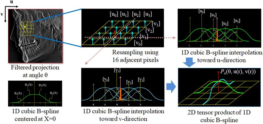
www.nature.com/scientificreports/

                                  Figure 1.  Overview of the proposed method for low-dose CBCT imaging.

                                  the parameter τ was set to 90% of the CDF histogram created by accumulating the intensity at each pixel of
                                  the log-transformed projection data. The parameter ε (in this study, we used ε = 3) is the scaling factor to make
                                  smaller weights for higher intensities, thereby reducing the blurring effect in high intensity regions.
                                      The NLTV objective function of Eq. (2) is minimized by the steepest gradient descent method with an adap-
                                  tive step size, which is expressed as follows:

                                                                                              ∇R Pj
                                                                                 t+1    t
                                                                                Pj = Pj −            ,                                         (4)
                                                                                             |∇R(P)|

                                                                                    =γ             Pj2 ,                                            (5)
                                                                                                j

                                  where λ is an adaptive parameter that controls the step size so that the smoothing degree is decreased according
                                  to an advancement in the iteration steps. By using the square root of all pixel elements updated in each steepest
                                  gradient descent step, this parameter is forced to progressively smaller values with an increase in the number
                                  of iterations. To avoid a local minimization due to an abrupt change, we use a scaling parameter γ and set it to
                                  an initial value of 1.0. If R(P) calculated at the current iteration step is larger than
                                                                                                                          that at the previous one, this
                                  value is linearly decreased by multiplying a constant value (rred = 0.8). ∇R Pj is the gradient of the objective
                                  function R(P) at the j-th indexed pixel. The root-sum-square of the gradient calculated at all pixels, |∇R(P)|, is
                                  required for the normalized gradient calculation. For clarity, we provide the following expression:

Scientific Reports |   (2021) 11:3681 |                https://doi.org/10.1038/s41598-021-83266-1                                                      3

                                                                                                                                                  Vol.:(0123456789)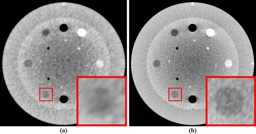
www.nature.com/scientificreports/
Figure 2. Comparison of filtered projection without (left) and with (right) the NLTV denoising algorithm.
Figure 3. Geometry of the projection data and notations for the voxel-driven backprojection step.
2P(u,v) − P(u−1,v) − P(u,v−1)
w(u,v) �� �2 � �2
P(u,v) − P(u−1,v) + P(u,v) − P(u,v−1)
� � ∂R(P) ∂R(P)
+w P(u,v) − P(u+1,v)
∇R Pj = = = (u+1,v)
2 , (6)
�
2
� � � �
∂Pj ∂P(u,v)
P(u+1,v) − P(u,v) + P(u+1,v) − P(u+1,v−1)
+w(u,v+1) � P(u,v) − P(u,v+1)
� �2 � �2
P(u,v+1) − P(u−1,v+1) + P(u,v+1) − P(u,v)
2
|∇R(P)| = ∇R Pj , (7)
j
The optimal number of iterations for the steepest gradient descent step was fine-tuned so that the noisy pixels
were minimized while preserving the striking features. In this study, the number of iterations for the steepest
gradient descent step was set to ten. In considering all the components mentioned above, we present the pseudo-
code of NLTV-based filtration as in Algorithm 1.
A circular pre-weighting factor was then applied on each NLTV denoised projection data to avoid the intensity
drop due to the cone angle effect. A 1D ramp filter was then applied to suppress the highest spatial frequency.
For the ramp filter, we used the product of the SL filter and raised the cosine window function in the frequency
domain. Each line parallel to the u-direction of the preweighted projection data was converted into the frequency
domain via 1D Fourier transformation. The Fourier transformed values were multiplied by the ramp filter.
By applying an inverse Fourier transformation, we could obtain the filtered projection data with the reduced
impulse noise. Figure 2 depicts the differences between filtered projections before and after applying the NLTV
denoising algorithm.
Scientific Reports | (2021) 11:3681 | https://doi.org/10.1038/s41598-021-83266-1 4
Vol:.(1234567890)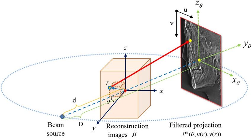
www.nature.com/scientificreports/

                                          Algorithm 1

                                            Calculate Gaussian kernel with a patch

                                            End For
                                                                                                ℎ

                                                  ←0

                                                                   ( )
                                                   End For

                                                              +                   ⁄ )
                                                                                         2ℎ20
                                               End For

                                                 ( )        ( )
                                            End For

                                                                                                    (6)

                                                      |   ( )| ←                                     (7)

                                               End For

                                                                           /|     ( )|
                                               End For
                                               While R(

                                                                   +
                                                                       |        ( )|
                                                  End For
                                               End While
                                               Update
                                            End For
                                          End For

                                  Voxel‑driven backprojector based on cubic B‑spline interpolation. Figure 3 shows the geometric
                                  information of the projection data and notations for voxel-driven backprojection calculation using the filtered
                                  projection data.
                                     Given a position vector r (or rx, ry, rz) of any voxel, corresponding positions (u(r) and v(r)) in the n-th projec-
                                  tion data at a given angle θ are obtained as follows:
                                                                                          P(θ , r) = P n (θ, u(r), v(r)),                           (8)
                                  where

Scientific Reports |   (2021) 11:3681 |                   https://doi.org/10.1038/s41598-021-83266-1                                                  5

                                                                                                                                                 Vol.:(0123456789)
www.nature.com/scientificreports/
Figure 4. Resampling process using 2D tensor product of 1D cubic B-spline interpolation from n-th filtered
projection.
rxθ
u(r) = , (9)
d + ryθ
rzθ
v(r) = , (10)
d + ryθ
T
Here, d is the source-to-axis distance, and the rotation vectors rxθ , ryθ , rzθ are calculated by applying the
rotation matrix through a given angle θ from the origin of the reconstruction images in the following manner:
� �
rxθ cosθ −sinθ 0 rx
ryθ = sinθ cosθ 0 ry , (11)
rzθ 0 0 1 rz
The final attenuation coefficient value, μ(r), at a position vector r is weighted and accumulated as
N
π
w(r)P n (θ, u(r), v(r)) , (12)
µ(r) = µ rx , ry , rz =
N
n=1
2
w(r) = d 2 / d + ryθ , (13)
where w(r) is the depth weighting and N is the total number of projection data. Every voxel has measurements
in all filtered projection data and is normalized by a uniform factor N in the backprojection step. As shown in
Fig. 4, P n (θ, u(r), v(r)) is represented as the 2D tensor product of a 1D cubic B-spline:
3
3
P n (θ, u(r), v(r)) = Bp u − up Bq v − vq P n θ, up , vq ,
(14)
p=0 q=0
where up = u + p − 1, vq = v + q − 1, and [·] is the floor function that maps a real number to the largest previous
integer. Bp and Bq correspond to the following cubic B-spline basis functions centered at X = 0:
B0 (X) = (2 − X)3 /6 if 1 ≤ X ≤ 2
B1 (X) = 3X3 − 6X2 + 4 /6
if 0 ≤ X < 1
3 2
(15)
B2 (X) = −3X − 6X + 4 /6 if − 1 ≤ X < 0
B3 (X) = (2 + X)3 /6 if − 2 ≤ X < −1.
In considering all the components mentioned above, we present the pseudo-code of cubic B-spline interpo-
lation-based backprojector as in Algorithm 2.
Scientific Reports | (2021) 11:3681 | https://doi.org/10.1038/s41598-021-83266-1 6
Vol:.(1234567890)www.nature.com/scientificreports/
Figure 5. Comparison between the same views of the high resolution reconstruction image generated by
applying FDK with (a) SL, (b) ATV, (c) NLTV, (d) SL + cubic B-spline, (e) ATV + cubic B-spline, and (f)
NLTV + cubic B-spline using the Catphan503 phantom. These images are displayed at window (width and level)
settings of (975, 0) HU.
Algorithm 2
Calculate rotation matrix M which maps voxel coordinate to projection coordinate
( )
( )
End For
( )
End For
( ) ( ) (14)
( ) ( )
End For
End For
Experimental studies. The Catphan503 (Phantom Laboratory, Salem, NY) was scanned using an Infinity™
linear accelerator system with XVI R5.0 (Elekta Limited, Stockholm, Sweden). The phantom includes various
modules for assessing the quality of 3D images. As the gantry rotates around the phantom, a series of CBCT
projections were acquired with 360° rotation under a small FOV protocol using a S20 collimator and an F0 filter.
Scientific Reports | (2021) 11:3681 | https://doi.org/10.1038/s41598-021-83266-1 7
Vol.:(0123456789)www.nature.com/scientificreports/
Figure 6. Comparison between the same views of the low resolution reconstruction image generated by
applying FDK with (a) SL, (b) ATV, (c) NLTV, (d) SL + cubic B-spline, (e) ATV + cubic B-spline, and (f)
NLTV + cubic B-spline using the Catphan503 phantom. These images are displayed at window (width and level)
settings of (975, 0) HU.
ROI Material of insert SL ATV NLTV SL + cubic B-spline ATV + cubic B-spline NLTV + cubic B-spline
1 Delrin™ 2.0 8.7 14.4 3.5 11.6 16.4
2 Teflon 4.2 14.3 23.6 7.0 18.2 25.9
3 Air 4.2 20.5 34.8 8.0 28.1 39.8
4 PMP 0.4 1.8 3.2 0.7 2.5 3.8
5 LDPE 0.1 0.2 0.4 0.1 0.3 0.5
6 Polystyrene 0.1 0.8 1.4 0.3 1.1 1.6
7 Air 4.3 21.0 35.9 8.3 29.1 41.9
Table 1. Comparison of CNRs at seven ROIs in the high resolution reconstructed image generated by six FDK
algorithms with low-dose projection data of the Catphan503 phantom.
The number of full scan projections was approximately 665. The size of each projection acquired on the image
receptor was 409.6 × 409.6 mm2, containing 1024 × 1024 pixels. The distance from the source to the detector and
the distance from the source to the axis were 1536 mm and 1000 mm, respectively. The low-dose acquisition
protocol had 100kVp with 0.1 mAs during each projection. Projections with different mAs settings were also
acquired for comparison. The reconstructed image of the phantom was generated with two resolution settings:
high resolution CBCT (512 × 512 × 200 voxels as well as 0.5 × 0.5 × 0.5 mm3 per each voxel) and low resolution
CBCT (256 × 256 × 100 voxels as well as 1.0 × 1.0 × 1.0 mm3 per each voxel). For comparison, a high-dose CBCT
was created as a benchmark image by applying a conventional FDK algorithm with projections acquired using
increased mAs setting (100 kVp and 1.6 mAs). The Hounsfield unit (HU) conversion was performed for all
Scientific Reports | (2021) 11:3681 | https://doi.org/10.1038/s41598-021-83266-1 8
Vol:.(1234567890)www.nature.com/scientificreports/
ROI Material of insert SL ATV NLTV SL + cubic B-spline ATV + cubic B-spline NLTV + cubic B-spline
1 Delrin™ 1.7 7.6 11.3 3.4 10.1 13.7
2 Teflon 4.2 13.2 20.6 6.5 17.8 24.2
3 Air 4.7 19.3 29.9 8.3 25.5 33.7
4 PMP 0.5 2.1 3.4 1.0 2.9 4.1
5 LDPE 0.1 0.3 0.4 0.1 0.3 0.5
6 Polystyrene 0.1 0.4 0.9 0.2 0.6 1.0
7 Air 4.0 19.7 31.6 7.8 27.3 37.1
Table 2. Comparison of CNRs at seven ROIs in the low resolution reconstructed image generated by six FDK
algorithms with low-dose projection data of the Catphan503 phantom.
SL ATV NLTV SL + cubic B-spline ATV + cubic B-spline NLTV + cubic B-spline
RMSE 181.0 69.0 62.4 112.6 64.3 61.4
Correlation 0.38 0.76 0.82 0.57 0.80 0.83
Table 3. Quantitative comparisons using two metrics in the high resolution reconstruction image generated
by six FDK algorithms with low-dose projection data of the Catphan503 phantom.
SL ATV NLTV SL + cubic B-spline ATV + cubic B-spline NLTV + cubic B-spline
RMSE 207.0 136.8 133.1 155.9 135.3 132.2
Correlation 0.43 0.77 0.82 0.57 0.80 0.82
Table 4. Quantitative comparisons using two metrics in the low resolution reconstruction image generated by
six FDK algorithms with low-dose projection data of the Catphan503 phantom.
SL ATV NLTV SL + cubic B-spline ATV + cubic B-spline NLTV + cubic B-spline
High resolution CBCT 95.8 269.4 1398.6 192.0 355.2 1485.8
Low resolution CBCT 79.7 251.4 1379.4 91.1 261.9 1390.0
Table 5. Computation time (seconds) of six FDK algorithms when creating high resolution and low resolution
CBCTs of the Catphan503 phantom.
reconstructed images. The CBCT image quality was quantified using three metrics (CNR, HU accuracy, and
correlation).
The accuracy of the HU number was assessed using the entire area of the CTP404 module of the phantom.
It has seven sensitometry inserts and the RMSE is calculated. The correlation and the CNR were also measured
using the same module. The correlation was calculated to evaluate the overall differences of the reconstructed
CBCT image versus benchmark CBCT images. For the RMSE and correlation measurement, a circular area
was selected to be measured only inside the phantom excluding the air area outside the phantom. For the CNR
measurement, the mean HU value and standard deviation were recorded by selecting seven ROIs within the
density insert and a central ROI.
Results
The performance of the NLTV denoised FDK reconstruction algorithm was evaluated with the Catphan503
phantom and compared with the Shepp–Logan (SL)-filtered FDK and anisotropic total variation (ATV)- denoised
FDK26. The ATV combines the edge stopping function used locally in an anisotropic diffusion fi lter27 for both
image enhancement and noise reduction. Figures 5 and 6 show a representative slice of the high resolution CBCT
(512 × 512 × 200 voxels) and low resolution CBCT (256 × 256 × 100 voxels) reconstructed from FDKs with SL,
ATV, and NLTV, as well as when adding the voxel-driven backprojector based on cubic B-spline interpolation on
filtered projections with SL, ATV, and NLTV, respectively. The artifacts were significantly suppressed in images
reconstructed by the proposed NLTV denoising compared to the other two algorithms. The CBCT images resa-
mpled with the cubic B-spline interpolation using 16 pixels (4 × 4) were smoother and had fewer interpolation
artifacts, resulting in slightly improved reconstruction accuracy for SL, ATV, and NLTV. The effect of this image
Scientific Reports | (2021) 11:3681 | https://doi.org/10.1038/s41598-021-83266-1 9
Vol.:(0123456789)www.nature.com/scientificreports/
Figure 7. Comparison of a representative slice of the reconstruction image generated by applying FDK using
high mAs projections and FDK with NLTV + cubic B-spline interpolation using low mAs projections. (a) high
resolution benchmark image, (b) high resolution CBCT produced by the proposed method, (c) low resolution
benchmark image, and (d) low resolution CBCT produced by the proposed method. These images are displayed
at window (width and level) settings of (2000, 0) HU.
quality improvement was the same for low resolution CBCT. In particular, the cubic B-spline interpolation still
visibly achieved substantial gains on all SL, ATV, and NLTV.
In addition, we calculated the contrast-to-noise ratio (CNR) at a selected region of interest (ROI) in the
reconstructed image. It was possible to conduct a comparison of the relative image contrast between the cor-
responding regions. Tables 1 and 2 provide a comparison of CNRs at seven ROIs in the high resolution and low
resolution reconstructed CBCT images obtained by six FDK algorithms. The proposed NLTV denoising shows
a better CNR in all ROIs compared to other two algorithms. Adding the cubic B-spline interpolation process
slightly improved the CNR to higher values for SL, ATV, and NLTV. Tables 3 and 4 list two quantitative meas-
ures (root-mean-square error (RMSE) and correlation) obtained from the high resolution and low resolution
reconstructed images based on the six FDK methods. The errors were computed against full projections with
a high mAs acquisition protocol (40 mA and 40 ms). The NLTV elicited a lower RMSE and a higher correla-
tion compared to the other algorithms. Adding the cubic B-spline interpolation produced the best results for
the Catphan503 phantom with a low noise scenario. Even in the SL and ATV, the cubic B-spline interpolation
could yield a lower RMSE and a higher correlation. Our proposed NLTV with the cubic B-spline interpolation
produced the lowest RMSE and the highest correlation. This relative superiority of the proposed method was
the same for the low resolution CBCT. The low resolution CBCT doubled the voxel size compared to the high
Scientific Reports | (2021) 11:3681 | https://doi.org/10.1038/s41598-021-83266-1 10
Vol:.(1234567890)www.nature.com/scientificreports/
Figure 8. Comparison of MIP of (a) high resolution benchmark CBCT images with a high mAs and high
resolution CBCT reconstruction images generated by applying FDK algorithms with (b) SL + cubic B-spline, (c)
ATV + cubic B-spline, and (d) NLTV + cubic B-spline using Catphan503 phantom acquired under a low mAs.
These images are displayed at window (width and level) settings of (1100, 500) HU.
resolution CBCT, leading to inferior feature details. This resulted in larger RMSE values and smaller CNR values
in the quantitative analysis.
Table 5 compares the computation times between the proposed method and other methods used in Figs. 5
and 6. Compared to SL and ATV, the computation time using the proposed NLTV denoising was approximately
14.5 times and 5.1 times longer for the high resolution CBCT generation and 17.3 times and 5.4 times longer for
the low resolution CBCT. It was influenced by the size and number of projections because NLTV was applied
to the projection data. Thus, the difference in calculation time due to high and low resolutions was not large.
On the other hand, the calculation time before and after applying the cubic B-spline interpolation required
approximately 90 s longer for high resolution CBCT and 10 s longer for the low resolution CBCT. Since the
cubic B-spline interpolation was applied after estimating the projection pixel for each voxel in the reconstructed
volume, it was affected by the reconstruction volume size. This resulted in a large difference in the calculation
time between the high and low resolution CBCTs.
Figure 7 shows the proposed method with projections acquired at low mAs levels and the conventional
FDK algorithm with projections acquired at high mAs levels (40 mA and 40 ms). These images enable us to
qualitatively judge the correspondence of line bars between the two reconstruction images. It was observed that
the proposed method shows a spatial resolution comparable to that of high-dose CBCT imaging through visual
inspection. Even with a high voxel size and low resolution, the visual effect was better than a low resolution
benchmark image with false artificial traces.
Scientific Reports | (2021) 11:3681 | https://doi.org/10.1038/s41598-021-83266-1 11
Vol.:(0123456789)www.nature.com/scientificreports/
Figure 9. Comparison of MIP of (a) low resolution benchmark CBCT images with a high mAs and low
resolution CBCT reconstruction images generated by applying FDK algorithms with (b) SL + cubic B-spline, (c)
ATV + cubic B-spline, and (d) NLTV + cubic B-spline using Catphan503 phantom acquired under a low mAs.
These images are displayed at window (width and level) settings of (1100, 500) HU.
Figures 8 and 9 compare the maximum intensity projections (MIP) of the reconstructed images. The MIP
image facilitates extraction of the highest value encountered along the corresponding viewing ray at each pixel
of the reconstructed images so that one can determine whether some regions with a high contrast are preserved
while reducing the noise. The proposed method showed that regions with remarkable features are well preserved
while reducing artifacts in the central region corresponding to the benchmark image compared to the other
two algorithms. After adding NLTV, the changes in the homogeneous region were smoother, whereas those in
the inhomogeneous regions were almost preserved. For the low resolution CBCT, a thin point feature showing
high contrast in the red ROI disappeared, even in the case of the benchmark image. However, it was found that
this thin feature was preserved in the reconstructed image when the proposed NLTV denoising was performed.
Figure 10 shows a visual inspection of the CBCTs generated by the post-processing approach of applying
NLTV to the FDK reconstructed image. In addition, it depicts the proposed method, i.e., the pre-processing
approach of applying FDK to the NLTV-denoised projections. We compared the low contrast resolution proper-
ties between the two approaches, as in the magnified area. The pre-processing strategy further revealed a higher
low contrast detection and detail-preserving effect compared to the post-processing strategy.
Scientific Reports | (2021) 11:3681 | https://doi.org/10.1038/s41598-021-83266-1 12
Vol:.(1234567890)www.nature.com/scientificreports/
Figure 10. Comparison between high resolution CBCT images generated by applying (a) NLTV on FDK
reconstructed images as a post-processing strategy and (b) FDK with NLTV-denoised projection data as a pre-
processing strategy. These Catphan503 phantom images are displayed at window (width and level) settings of
(750, 0) HU.
Discussion
CBCT reconstruction from low mAs has been challenging. X-ray tubes produce photons via electron bombard-
ment of a metallic anode. The number of photons is determined by the current across the tube (mA) and the
exposure time (s), which are sometimes multiplied together as mAs. Decreasing the mAs decreases the number
of electrons hitting the anode, and consequently, the number of photons generated by the tube decreases lin-
early. This decreases the number of photons reaching the detector, reducing the signal-to-noise ratio (SNR) of
the projection data.
The total variation (TV) transform was considered to mitigate the noise imprinted on the projection data,
but it tended to keep the edge information too smooth by uniformly penalizing the local image gradient. To
overcome this limitation, ATV was proposed to reduce the blurriness at edge regions by deriving the anisotropic
edges expressed as the exponential function of the adaptively weighted local image gradient of the projection
data. The limitation of ATV is that the capability of deriving local edge information is restricted by the quality of
projection data. The projection data acquired at low mAs settings suffer from severe noise. Thus, it is difficult to
develop a local edge detection operator that reliably finds features with smaller details and is noise-insensitive.
Conversely, the NLTV can help overcome this shortcoming by utilizing more global searches and non-uniform
weights depending on the similarities between non-local patches. Combining the cubic B-spline interpolation-
based backprojector allows the NLTV denoising-based FDK algorithm to be further enhanced and obtain more
precise low-dose CBCT reconstruction images. The reason for such a performance improvement was that the
CBCT reconstructed from conventional FDK with SL, ATV, and NLTV were based on nearest neighbor (NN)
interpolation-based backprojector. NN is the simplest and fastest interpolation method, but it can introduce
significant distortion. The cubic B-spline interpolation is more complex than the NN method and is thus more
computationally expensive. For an unknown pixel in the projection data, the influence range is extended to16
adjacent pixels. Then the pixel value is calculated as 16 pixels based on the distance. More complex improved
interpolation methods such as cubic B-spline make the interpolation curve smoother. Thus, there are no discrete
defects and the high-frequency components are faded. This characteristic provides better visual effects without
false artificial traces even at high voxel sizes and low resolutions.
We applied our proposed approach, the combination of NLTV and cube B-spline interpolation, to phantom
data and compared its performance with the results from SL and ATV filtrations in terms of visual inspection,
RMSE, CNR, and correlation. Reconstructions performed by the proposed method indicated that a higher image
quality could be achieved with projection data acquired under a lower mAs protocol. We also determined that
the proposed method shows a CNR with a spatial resolution comparable to those of images reconstructed using
projections acquired from a high-dose protocol. Moreover, NLTV denoising yields filtered projection data with
a greatly reduced noise using non-local patches. The cubic B-spline interpolation process slightly improved the
reconstruction accuracy on SL, ATV, and NLTV, as well as the image clarification. All these results indicate that
the proposed algorithm not only achieves a potential radiation dose reduction in the repeated CBCT scans, but
also eliminates noise effectively without heavily compromising the striking features.
Technically, compared with the ATV transform, the proposed technique might increase the computational
cost due to the larger search area when computing the weight function. In this work, to balance the reconstructed
image quality with the computational burden, the search area was limited to 21 × 21 pixels around each pixel. The
extra computational burden is related to the time elapsed for the backprojector with cubic B-spline interpolation.
Scientific Reports | (2021) 11:3681 | https://doi.org/10.1038/s41598-021-83266-1 13
Vol.:(0123456789)www.nature.com/scientificreports/
In our implementation, OpenMP was used to parallelize the proposed algorithm on an Intel Xeon CPU with 24
physical cores and 48 logical processors. Therefore, the proposed algorithm can be extended and accelerated by
using a G PU28. The number of iterations for the NLTV minimization was determined to be ten, however, this
value may not be optimal. Among the datasets used, we observed better reconstructed images with suppressed
noise and preserved edges when the number of iterations was ten.
The same magnitude of imaging dose reduction can be achieved by reducing the number of projections while
maintaining the mAs setting. However, this approach assumes fast gantry rotation. The maximum gantry speed
of clinically used CBCT scanners is still limited to 1 rpm or 6°/s. Thus, low mAs acquisition may be a better
option for imaging dose reduction than sparse view acquisition in practical aspects.
The NLTV denoising method can be extended to various applications. It can be used as an image fidelity
term in compressed sensing-based a pproaches23. NLTV-based FDK reconstruction images can be used as an
initial guess image for iterative r econstruction10,29. In general, it has been observed that the better the initial
guess image when using an iterative reconstruction algorithm, the faster the convergence and CBCT images
that can be created with a high contrast. In addition, a ray-driven backprojector can be combined with N LTV28.
In conclusion, an improved FDK reconstruction algorithm for low-dose CBCT imaging has been developed
by adding non-local total variation (NLTV) denoising in the filtering process and a voxel-driven backprojector
based on cubic-B spline interpolation. The proposed approach allows the conventional FDK algorithm to be
used for low mAs image reconstruction without requiring iterative reconstruction algorithms, which are com-
putationally demanding. Moreover, substantial reductions in radiation exposure associated with the low mAs
projection acquisition can facilitate wider practical applications of IGRT using daily online CBCT imaging with
corrections for setup errors.
Data availability
All data generated or analyzed during this study are included in the article.
Received: 12 August 2020; Accepted: 28 January 2021
References
1. Nabavizadeh, N. et al. Image guided radiation therapy (IGRT) practice patterns and IGRT’s impact on workflow and treatment
planning: results from a national survey of American Society for Radiation Oncology members. Int. J. Radiat. Oncol. Biol. Phys.
94, 850–857 (2016).
2. Fuchs, F. et al. Interfraction variation and dosimetric changes during image-guided radiation therapy in prostate cancer patients.
Radiat. Oncol. J. 37, 127 (2019).
3. Yoon, J., Park, K., Kim, J. S., Kim, Y. B. & Lee, H. Skin dose comparison of CyberKnife and helical tomotherapy for head-and-neck
stereotactic body radiotherapy. Prog. Med. Phys. 30, 1–6 (2019).
4. Han, Y. Current status of proton therapy techniques for lung cancer. Radiat. Oncol. J. 37, 232 (2019).
5. Lu, L. et al. Intra-and inter-fractional liver and lung tumor motions treated with SBRT under active breathing control. J. Appl. Clin.
Med. Phys. 19, 39–45 (2018).
6. Yang, Y., Schreibmann, E., Li, T., Wang, C. & Xing, L. Evaluation of on-board kV cone beam CT (CBCT)-based dose calculation.
Phys. Med. Biol. 52, 685 (2007).
7. Yoganathan, S. et al. Evaluating the image quality of cone beam CT acquired during rotational delivery. Br. J. Radiol. 88, 20150425
(2015).
8. Alaei, P. & Spezi, E. Imaging dose from cone beam computed tomography in radiation therapy. Phys. Med. 31, 647–658 (2015).
9. Wang, J., Li, T., Liang, Z. & Xing, L. Dose reduction for kilovotage cone-beam computed tomography in radiation therapy. Phys.
Med. Biol. 53, 2897 (2008).
10. Lee, H. et al. Improved compressed sensing-based cone-beam CT reconstruction using adaptive prior image constraints. Phys.
Med. Biol. 57, 2287 (2012).
11. Chen, G. H., Tang, J. & Leng, S. Prior image constrained compressed sensing (PICCS): a method to accurately reconstruct dynamic
CT images from highly undersampled projection data sets. Med. Phys. 35, 660–663 (2008).
12. Feldkamp, L., Davis, L. & Kress, J. Practical cone-beam algorithm. J. Opt. Soc. Am. A 1, 612–619 (1984).
13. Ahmadi, R., Farahani, J. K., Sotudeh, F., Zhaleh, A. & Garshasbi, S. Survey of image denoising techniques. Life Sci. J. 10, 753–755
(2013).
14. Motwani, M. C., Gadiya, M. C., Motwani, R. C. & Harris, F. C. Survey of image denoising techniques in Proceedings of GSPX
27-302004.
15. Yuan, N. et al. Convolutional neural network enhancement of fast-scan low-dose cone-beam CT images for head and neck radio-
therapy. Phys. Med. Biol. 65, 035003 (2020).
16. Chen, L., Liang, X., Shen, C., Jiang, S. & Wang, J. Synthetic CT generation from CBCT images via deep learning. Med. Phys. 47,
1115–1125 (2020).
17. Kida, S. et al. Cone beam computed tomography image quality improvement using a deep convolutional neural network. Cureus
10, e2548 (2018). https://doi.org/10.7759/cureus.2548.
18. Chen, H. et al. Low-dose CT via convolutional neural network. Biomed. Opt. Express 8, 679–694 (2017).
19. Lee, H., Lee, J., Kim, H., Cho, B. & Cho, S. Deep-neural-network-based sinogram synthesis for sparse-view CT image reconstruc-
tion. IEEE Trans. Radiat. Plasma Med. Sci. 3, 109–119 (2018).
20. Liang, X. et al. Generating synthesized computed tomography (CT) from cone-beam computed tomography (CBCT) using Cycle-
GAN for adaptive radiation therapy. Phys. Med. Biol. 64, 125002 (2019).
21. Sidky, E. Y., Lorente, I., Brankov, J. G. & Pan, X. Do CNNs solve the CT inverse problem. IEEE Trans. Biomed. Eng. (2020). https
://doi.org/10.1109/TBME.2020.3020741.
22. Sidky, E. Y. & Pan, X. Image reconstruction in circular cone-beam computed tomography by constrained, total-variation minimiza-
tion. Phys. Med. Biol. 53, 4777 (2008).
23. Kim, H. et al. Non-local total-variation (NLTV) minimization combined with reweighted L1-norm for compressed sensing CT
reconstruction. Phys. Med. Biol. 61, 6878 (2016).
24. Kim, K., El Fakhri, G. & Li, Q. Low-dose CT reconstruction using spatially encoded nonlocal penalty. Med. Phys. 44, e376–e390
(2017).
Scientific Reports | (2021) 11:3681 | https://doi.org/10.1038/s41598-021-83266-1 14
Vol:.(1234567890)www.nature.com/scientificreports/
25. Sohn, J. J. et al. Analytical low-dose CBCT reconstruction using non-local total variation regularization for image guided radiation
therapy. Front. Oncol. 10, 242 (2020).
26. Lee, H., Yoon, J. & Lee, E. Anisotropic total variation denoising technique for low-dose cone-beam computed tomography imaging.
Prog. Med. Phys. 29, 150–156 (2018).
27. Perona, P. & Malik, J. Scale-space and edge detection using anisotropic diffusion. IEEE Trans. Pattern Anal. Mach. Intell. 12, 629–639
(1990).
28. Park, H.-G., Shin, Y.-G. & Lee, H. A fully GPU-based ray-driven backprojector via a ray-culling scheme with voxel-level paral-
lelization for cone-beam CT reconstruction. Technol. Cancer Res. Treat. 14, 709–720 (2015).
29. Lee, H., Fahimian, B. P. & Xing, L. Binary moving-blocker-based scatter correction in cone-beam computed tomography with
width-truncated projections: proof of concept. Phys. Med. Biol. 62, 2176 (2017).
Author contributions
Conception, design, and drafting of the manuscript were performed by H.L., B.J.M., and I.J.L. Data collection
and interpretation were performed by J.P. and Y.C., K.R.P. reviewed the contents. All authors read and approved
the final manuscript.
Funding
This study was supported by the 2020 Research Grant of Gangnam Severance Hospital Research Committee
(DHHD000067), by the Basic Science Research Program through the National Research Foundation of Korea
funded by the Ministry of Education (2019R1I1A1A01062157), and by a grant of the Korea Health Technology
R&D Project through the Korea Health Industry Development Institute (KHIDI) funded by the Ministry of
Health & Welfare, Republic of Korea (HI19C1330).
Competing interests
The authors declare no competing interests.
Additional information
Correspondence and requests for materials should be addressed to B.J.M. or I.J.L.
Reprints and permissions information is available at www.nature.com/reprints.
Publisher’s note Springer Nature remains neutral with regard to jurisdictional claims in published maps and
institutional affiliations.
Open Access This article is licensed under a Creative Commons Attribution 4.0 International
License, which permits use, sharing, adaptation, distribution and reproduction in any medium or
format, as long as you give appropriate credit to the original author(s) and the source, provide a link to the
Creative Commons licence, and indicate if changes were made. The images or other third party material in this
article are included in the article’s Creative Commons licence, unless indicated otherwise in a credit line to the
material. If material is not included in the article’s Creative Commons licence and your intended use is not
permitted by statutory regulation or exceeds the permitted use, you will need to obtain permission directly from
the copyright holder. To view a copy of this licence, visit http://creativecommons.org/licenses/by/4.0/.
© The Author(s) 2021
Scientific Reports | (2021) 11:3681 | https://doi.org/10.1038/s41598-021-83266-1 15
Vol.:(0123456789)You can also read