SEMANTIC SEGMENTATION OF TERRESTRIAL LIDAR DATA USING CO-REGISTERED RGB DATA - The International Archives of the ...
←
→
Page content transcription
If your browser does not render page correctly, please read the page content below
The International Archives of the Photogrammetry, Remote Sensing and Spatial Information Sciences, Volume XLIII-B2-2021
                                                  XXIV ISPRS Congress (2021 edition)

               SEMANTIC SEGMENTATION OF TERRESTRIAL LIDAR DATA USING
                             CO-REGISTERED RGB DATA

                                            E. Sanchez Castillo1 ∗, D. Griffiths1 , J. Boehm1
                           1
                        Dept. of Civil, Environmental & Geomatic Engineering, University College London,
                  Gower Street, London, WC1E 6BT UK - (erick.castillo.19, david.griffiths.16, j.boehm)@ucl.ac.uk

                                                      Commission II, WG II/3

KEY WORDS: terrestrial laser scanning, point cloud, panoramic image, semantic segmentation, convolutional neural network

ABSTRACT:

This paper proposes a semantic segmentation pipeline for terrestrial laser scanning data. We achieve this by combining co-registered
RGB and 3D point cloud information. Semantic segmentation is performed by applying a pre-trained off-the-shelf 2D convolutional
neural network over a set of projected images extracted from a panoramic photograph. This allows the network to exploit the
visual image features that are learnt in a state-of-the-art segmentation models trained on very large datasets. The study focuses
on the adoption of the spherical information from the laser capture and assessing the results using image classification metrics.
The obtained results demonstrate that the approach is a promising alternative for asset identification in laser scanning data. We
demonstrate comparable performance with spherical machine learning frameworks, however, avoid both the labelling and training
efforts required with such approaches.

                      1. INTRODUCTION                                 (CNNs). Our multi-stage pipeline first starts with the extraction
                                                                      of a panoramic image from a TLS acquired point cloud. Next,
Over the past decade, the construction and real estate sectors        we compute tangential images in a perspective projection which
have increasingly used Terrestrial Laser Scanners (TLS) to cap-       can be fed into a CNN to map RGB values to per-pixel labels.
ture and document building interiors. This process usually de-        Finally, we project the label map back to the point cloud to
livers a dense, high-quality point cloud, which can serve as          obtain per-point labels. Through a hyperparameter grid search
the basis for remodelling and asset management. Furthermore,          we find that our method can be used to obtain a competitive
modern instruments not only capture the 3D positions of in-           semantic segmentation of point clouds leveraging only a pre-
terior surfaces, but also colour information from panoramic           trained off-the-shelf 2D CNN without any additional labelling
photographs, making it possible for a point cloud to be reasoned      or domain adaptation.
from both its spatial and photometric qualities. A key task in
point cloud scene understanding is assigning an object label for      Empirically we show that despite the raw image data being in an
every point, often referred as either per-point classification or     equirectangular projection, CNNs trained using the more com-
semantic segmentation. In this work we adopt the latter.              mon rectilinear projection produce respectable labels using our
                                                                      approach. Our pipeline therefore makes data captured by polar
In recent years, a surge of deep learning approaches for point        devices, such as a TLS, compatible with any standard CNN-
cloud semantic segmentation have been proposed. Neverthe-             based image segmentation architecture.
less, the problem is still considered hard. This can be accred-
ited to a number of reasons. Firstly, point clouds are typically                          2. RELATED WORKS
unordered, and sparse data types. This prevents normal con-
volution kernels, which assume discrete structured data, from         The process of assigning per-point classification labels to point
being effective. As a result, deep learning based 2D approaches       clouds has a rich history. Traditionally, success has been owed
typically remain more mature. Despite great progress in ad-           to supervised machine learning based techniques. As a single
dressing this problem (Qi et al., 2017b; Hermosilla et al., 2018;     point does not contain enough information to determine its la-
Thomas et al., 2019), another issue looms. Modern deep learn-         bel, researchers explore methods to encompass local neighbour-
ing based methods require very large labelled datasets, however,      hood context. Demantké et al. (2011), Weinmann et al. (2015)
such datasets for 3D data are typically not available at the same     and others demonstrated the effectiveness of explicitly encod-
scale as that for their 2D counterparts.                              ing features computed from a points local neighbourhood. Fea-
                                                                      tures such as linearity, planarity and Eigenentropy are calcu-
In light of such limitations, we instead ask the question, can 3D
                                                                      lated for each point and passed into a Random Forest classifier.
point cloud semantic segmentation be achieved using only 2D
                                                                      This can be performed at scale (Liu and Boehm, 2015). Other
models? Ultimately allowing us to exploit existing 2D CNN
                                                                      feature sets such as Fast Point Feature Histograms (FPFH)
architectures and massive manually labelled 2D datasets.
                                                                      (Rusu et al., 2009) and Color Signature of Histogram of Orient-
In answering this, we propose a methodology which projects            ations (SHOT) (Salti et al., 2014) have also shown promising
3D data with co-registered RGB data into 2D images which can          results.
be consumed by standard 2D Convolutional Neural Networks
                                                                      More recently, there has been a surge of deep learning based
∗   Corresponding author                                              approaches (Griffiths and Boehm, 2019). The seminal work of

                                                 This contribution has been peer-reviewed.
                  https://doi.org/10.5194/isprs-archives-XLIII-B2-2021-223-2021 | © Author(s) 2021. CC BY 4.0 License.             223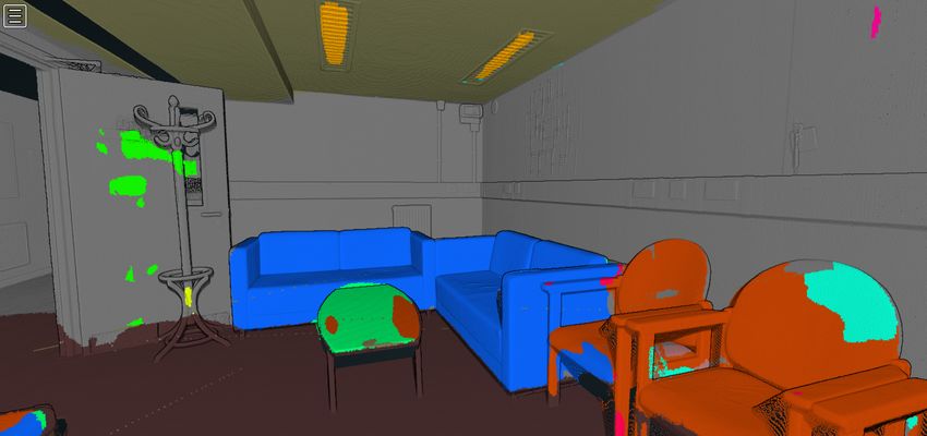
The International Archives of the Photogrammetry, Remote Sensing and Spatial Information Sciences, Volume XLIII-B2-2021
                                                XXIV ISPRS Congress (2021 edition)

PointNet (Qi et al., 2017a) demonstrated the compatibility of        i.e. Rn×k → Rn×1 where n is the number of points in P and
deep learning with such problems. However, PointNet did not          k ∈ Rx,y,z,r,g,b (although k can include other sensor features
exploit local neighbourhood features like those explicitly en-       such as intensity). Whilst in remote sensing and photogram-
coded in early works. PointNet++ (Qi et al., 2017b) showed that      metry this problem is typically referred to as (per-point) clas-
by combining a PointNet with local neighbourhood grouping            sification, we use the term semantic segmentation common in
and sampling module, results could be significantly improved.        image processing as these are the networks we use for creating
More recent research looks at developing convolution kernels         the label mapping function f : Rn×k → Rn×1 .
(which experienced unprecedented success in the 2D domain)
that are capable of working in the unordered, sparse and con-        Our methodology can be split into the following primary pro-
tinuous domain where the point cloud exists. Examples such           cesses. First, a point cloud P with corresponding RGB image
as Monte Carlo Convolutions (Hermosilla et al., 2018), Kernel        data I ∈ Rh×w×3 is captured using a survey-grade TLS. Such
Point Convolutions (Thomas et al., 2019) and PointConv (Wu           scanners are two-axis polar measurement instruments and ac-
et al., 2019) address this.                                          quire quasi regular samples on the two axes, effectively cre-
In the 2D domain researchers have developed methods for pro-         ating a regular grid in the polar space. This representation is
cessing spherical images. For example, the spherical cross-          also commonly used in panoramic imaging and is referred to as
correlation and generalised Fourier transform algorithms in Co-      equirectangular. The scanner hardware or associated software
hen et al. (2018), the adaptation of different convolution lay-      warps the image data captured alongside the point cloud into
ers in Yu and Ji (2019), or transforming encoders and decoders       this projection. The resulting panoramic colour images can be
for understanding the geometry variance derived from the input       extracted using open standard file formats.
equirectangular panoramic image in Zhao et al. (2018b). Zhao
et al. (2018a) improved spherical analysis for equirectangular       Next, we convert the information of the panoramic image I
images by creating networks that can iterate between image           to tangential images I T to simulate a rectilinear lens. This
sectors and classify panoramas with significant performance          projection is not a valid transformation for the complete pan-
and speed, which is comparable to classic two-dimensional net-       oramic image, and therefore we create a sequence of over-
works.                                                               lapping partial images. The position of the tangential images
                                                                     is determined using spherical grid sequence intervals, creat-
As it is possible for 3D point clouds to be projected into a 2D
                                                                     ing an almost equal distribution over the spherical space such
spherical domain, naturally, approaches have been proposed
                                                                     that I T = {I1t . . . Int }. We then obtain per-pixel labels I s ∈
to exploit the spherical 2D CNNs for 3D semantic segmenta-
                                                                     Rh×w×1 by utilising a semantic segmentation CNN S such that
tion. Jiang et al. (2019), parse spherical grids approximated to
                                                                     Iis = S(Iit ). All partial rectilinear label images Iis are then
a given underlying polyhedral mesh, using what the author calls
                                                                     projected back to the original panoramic projection, allowing
”Parameterised Differential Operators”, which are linear com-
                                                                     the final label map I C to be created using the confidence scores
binations of differential operators that avoid geodetic computa-
                                                                     obtained by the semantic segmentation process. In our exper-
tions and interpolations over the spherical projection. Similarly,
                                                                     iments S is a pre-trained UperNet model (Xiao et al., 2018)
Zhang et al. (2019) propose an orientation-aware semantic seg-
                                                                     which was trained on the rectilinear based ADE20K dataset
mentation on icosahedral spheres.
                                                                     (Zhou et al., 2017). Finally, we map the class labels I C → P
Concurrent research has also been present in the autonomous          using the co-registration matrix, assigning per-point labels. Fig-
driving domain. Wu et al. (2018); Wang et al. (2018) transform       ure 1 gives a graphical overview of the process. In the following
3D scanner data into 2D spherical image which is fed into a          sections we will discuss each stage in detail.
2D CNN, before unprojecting labels back to the original point
cloud. These methods are typically a lot faster than purely 3D
approaches as projection and 2D convolutions are much faster
than 3D neighbourhood searches required by geometric-based
approaches. Similar to our work, Tabkha et al. (2019) perform
semantic segmentation using a Convolutional Neural Network
(CNN) on RGB images derived by projecting coloured 3D point
clouds. However, our work differs from these approaches as we
do not use an unordered point cloud as the representation for the
LiDAR data. Instead, we use the ordered panoramic represent-
ation that is generated by polar measuring devices such as TLS.
On the downside this restricts our approach to single scans cap-
tured with static TLS and excludes e.g., mobile scanners.
Also similar to our work, Eder et al. (2020) divide a spherical
panoramic image into tangential icosahedral planes and the pro-
ject individual perspective images. This allows each image to
be fed into a pre-trained 2D semantic segmentation CNN. Fur-
thermore, Eder et al. (2020) obtained comparable results using
standard CNNs to more specialised spherical CNNs.

                    3. METHODOLOGY
                                                                          Figure 1. This diagram shows the proposed semantic
Given a point cloud P ∈ Rn×k captured using a polar-based             segmentation process using panoramic images from TLS data.
TLS scanner, we aim to assign a per-point object class label

                                                This contribution has been peer-reviewed.
                 https://doi.org/10.5194/isprs-archives-XLIII-B2-2021-223-2021 | © Author(s) 2021. CC BY 4.0 License.              224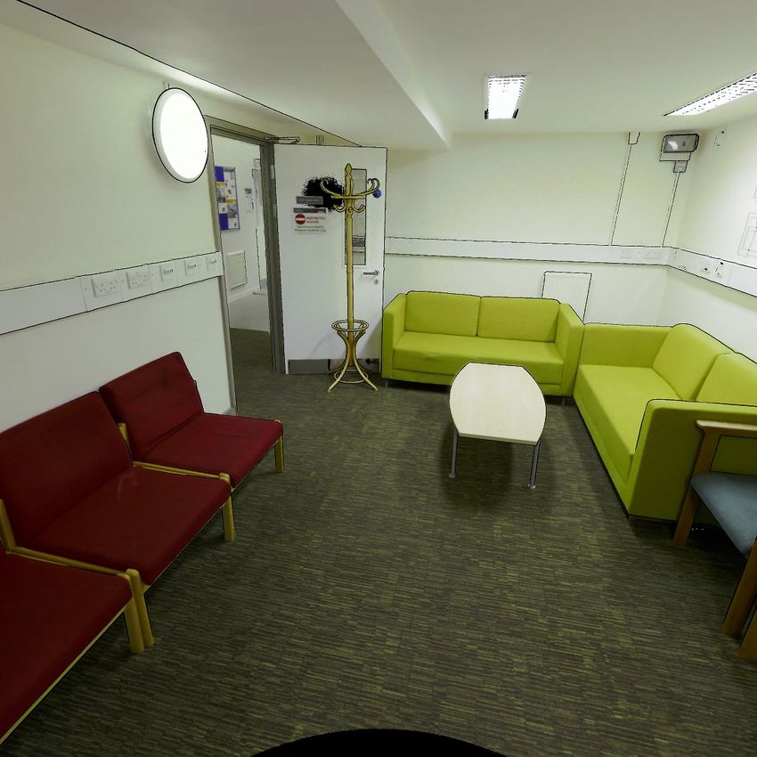
The International Archives of the Photogrammetry, Remote Sensing and Spatial Information Sciences, Volume XLIII-B2-2021
XXIV ISPRS Congress (2021 edition)
3.1 Data acquisition
Our scanner data (P and I ) in this project was collected using a
Leica RTC360 TLS. This system (along with many other com-
mercially available systems) captures 3D measurements in a
structured sequence. As mentioned above it acquires the points
over a quasi-regular grid in the polar space. This polar grid
is directly represented as a two-dimensional matrix. This en-
ables the projection of 3D point cloud data from a polar to an
equirectangular projection. Effectively transforming the cap-
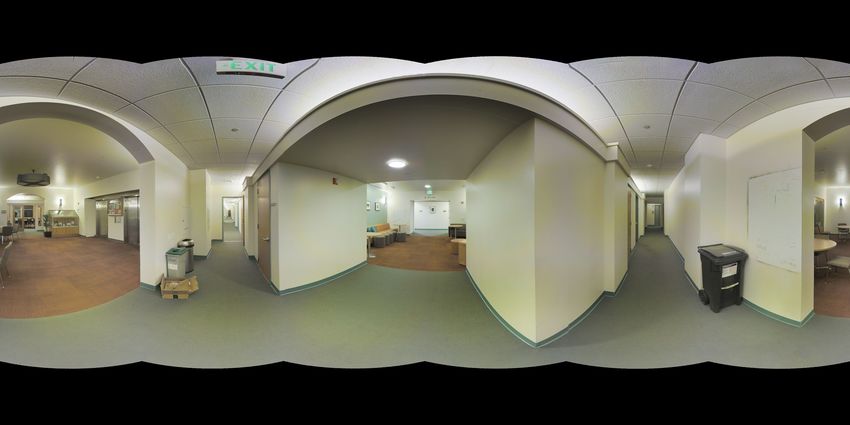
tured data into a panoramic image (Figure 2 Row 1). This
representation of TLS data is long established for image pro-
cessing and object extraction (Boehm and Becker, 2007; Eysn
et al., 2013).
We processed all data with the manufacturer software, export-
ing the point cloud to a grid-type separator file format that pre-
serves the orientation header of the scan position and each cor-
responding scanned point on the ordered grid. We utilise this
raster grid to extract the panoramic image directly. The final
resolution of our panoramic image is (20, 334 × 8, 333). This
is generated from a maximum of 169, 443, 222 points (as lim-
ited by the TLS), however, in practice much fewer points are
actually captured due to lack of returns from angular surfaces,
windows etc.
3.2 Rectilinear projection
With the TLS capture described above having a spherical
equidistant subdivision, the creation of an equirectangular pro-
jection is trivial, interpreting the data as a raster. As this projec-
tion is neither equal-area nor conformal, there are distortions in
the resulting panoramic image. To address the spherical distor-
tion, we need to define a rectilinear projection for tangential im-
ages and a subdivision method from where the tangential points
will be defined for each individual projection.
The mathematical foundations used in this reprojection process
are detailed as follows, extracted from Weisstein (2018). Given
a point pi ∈ P with a latitude and longitude (λ, φ), the trans-
formation equations for the creation of a tangent plane at that
point, with a projection with central longitude λ0 and central Figure 2. Data at different stages of the pipeline. Row 1
latitude φ1 are given by: Panorama image created from TLS point cloud with the
co-registered RGB information. Row 2 Example of tangential
image in rectilinear projection and segmentation result. Row 3
cos φ sin (λ − λ0 ) The semantic segmentation output re-projected from tangential
x= (1)
cos c to equirectangular. The full map is given in Figure 6. Row 4
Point cloud rendering with labels from merged equirectangular
segmentation map.
cos φ1 sin φ − sin φ1 cos φ cos (λ − λ0 )
y= (2)
cos c
To create the lattice, the function of this sequence for the sym-
Where c is the angular distance of the point (x, y) from the metrical points n is described as n = 2N + 1 where N is any
projection centre, given by: natural number defining the desired interval subdivision and the
integer i range from −N to +N . The spherical coordinates of
ith point are:
cos c = sin φ1 sin φ + cos φ1 cos φ cos (λ − λ0 ) (3)
2i
lati = arcsin (4)
Knowing the image size and the corresponding field of view 2N + 1
(FOV) angle for the respective c, we can generate individual
images I T from the full-dome panorama I . The latitude and
longitude (λ, φ) positions of the spherical intervals are defined loni = 2πiΦ−1 (5)
by the golden ratio angle separation, where the generative spir-
als of a Fibonacci lattice turn between consecutive points along where: √
a symmetrical spiral sphere (Gonzalez, 2009). Φ = 1 + Φ−1 = (1 + 5)/2 ' 1.618 (6)
This contribution has been peer-reviewed.
https://doi.org/10.5194/isprs-archives-XLIII-B2-2021-223-2021 | © Author(s) 2021. CC BY 4.0 License. 225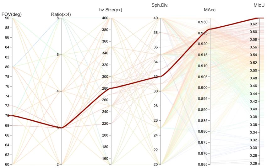
The International Archives of the Photogrammetry, Remote Sensing and Spatial Information Sciences, Volume XLIII-B2-2021
                                                 XXIV ISPRS Congress (2021 edition)

and Φ is the golden ratio.                                                 With the central longitude λ0 , central latitude φ1 , φ and λ being
                                                                           the resulting latitude and longitude for each reprojected pixel
The result of this projection, which is also referred to as                (x, y), respectively. ρ and c are defined as:
gnomonic projection, is a quasi perspective image Iit (Figure
2 Row 2) which is equivalent to an image captured by a camera                                             p
with a rectilinear lens. Typical cameras available today try to                                      ρ=       x2 + y 2                     (9)
achieve such a projection. As a result the projected images are
of the same projection as those of most large scale benchmark
datasets used to train 2D ML models.
                                                                                                      c = tan−1 ρ                         (10)
3.3   Semantic segmentation
                                                                           The resulting image has the corresponding order of latitude and
At the centre of our pipeline is a deep learning based semantic            longitude of the spherical subdivision (Figure 2 Row 3).
segmentation network S which maps a single tangential image
to a probability class map S : IiT → Iis (Figure 3). A key                 3.5   Panoramic Label Map
benefit of our pipeline is that it is compatible with any choice
of S . In such a fast moving field this allows the user to drop            Following the processing methodology, it is necessary to re-
in the current best performing network implementation. In this             create a full resolution panoramic label image I C from the
work we opt for the widely used UPerNet network (Xiao et al.,              overlapping tangential semantic segmentation maps (i.e. Iit ∈
2018) as an example.                                                       I C → I C ). To achieve this, we adopt a winner-take-all ap-
                                                                           proach from the corresponding pixel confidence scores C s ∈
We choose this network for several reasons. Firstly, the net-              C C . The final output map for any redundant pixels is therefore:
work performs competitively on computer vision benchmarks.
Next, the authors offer an easy-to-use publicly available imple-
mentation. Lastly, the authors release pre-trained weights on                            I C (λ, φ) = max[Cis (λ, φ), Cjs (λ, φ)]         (11)
                                                                                                       i,j
the ADE20K indoor scene parsing dataset, which contains all
of the objects present in our datasets.
                                                                           3.6   Point cloud semantic segmentation
We note, that whilst any 2D CNN semantic segmentation net-
work can be used in our pipeline, it is important that the user            As a final step we map the equirectangular label map onto the
also has access to the prediction confidence scores Cis ∈ C C (as          original point cloud (i.e. I C → P ). This is easily achieved by
output from the final prediction probability distribution). These          storing the original mapping P → I (Section 3.1). Using the
values are used to handle redundant label when recomposing                 reverse of this mapping we simply assign each point pi ∈ P its
Iis ∈ I C → I C . This is discussed in detail in Section 3.4.              corresponding value from I C . A rendering of the point cloud
                                                                           with label colours is shown in Figure 2 Row 4.

                                                                                                     4. RESULTS

                                                                           We test our methodology outlined in Section 3 for a range
                                                                           of configurations. Furthermore, we evaluate our approach on
                                                                           both an internal dataset and a sample from the common 2D3DS
                                                                           benchmark dataset (Armeni et al., 2017).
   Figure 3. Projected tangential image (left), visualisation of
      UPerNet semantic segmentation classes (centre) and                   4.1   Performance metrics
 corresponding confidence map where darker is more confident
                                                                           It is important to define the metrics used to evaluate our pro-
                            (right).
                                                                           posed pipelines performance. Whilst the 2D3DS dataset con-
                                                                           tains labels, our internal dataset did not. It is therefore neces-
3.4   Reprojection                                                         sary to label the ground truth data. As we are not using the
                                                                           dataset for training a CNN, all data is test data, and as such,
After obtaining the semantically segmented images Iis ∈ I C                we do not require a large dataset. All data was therefore manu-
and the confidence matrix associated to each tangential position           ally annotated using standard image processing software with a
(λ, φ), it is necessary to warp back the images to the equirect-           graphical user interface.
angular projection, in order to obtain a new set of panoramic
images for the posterior unification process. The inverse trans-           To evaluate each scenario’s performance, we opt for the widely
formation equations, having a pixel coordinate (x, y), are given           used Intersection over Union metric (Everingham et al., 2010),
by:                                                                        averaged over all classes (mIoU). In practise we compute the
                                                                           IoU over the N ×N confusion matrix C , where N is number of
                                                                           classes (21 in our case). Let cij be a single entry in C , where cij

                    −1                   y sin c cos φ1                    is a number of sampled from the ground truth class i predicted
          φ = sin         cos c sin φ1 +                             (7)   as class j , then the per-class IoU can be computed as:
                                                ρ

                                                                                                                    cii
                                                                                            IoUi =                                        (12)

                                           x sin c
      λ = λ0 + tan−1
                                                                                                             P            P
                                                                     (8)                             cii +          cij +   cki
                               ρ cos φ1 cos c − y sin φ1 sin c                                               j6=i        k6=i

                                               This contribution has been peer-reviewed.
                https://doi.org/10.5194/isprs-archives-XLIII-B2-2021-223-2021 | © Author(s) 2021. CC BY 4.0 License.                       226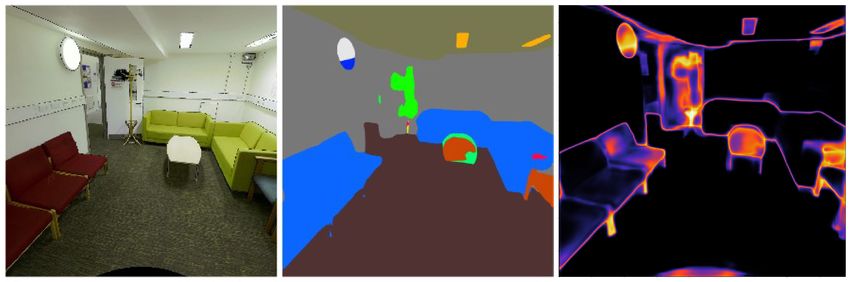
The International Archives of the Photogrammetry, Remote Sensing and Spatial Information Sciences, Volume XLIII-B2-2021
XXIV ISPRS Congress (2021 edition)
mIoU is then:
N
1 X
mIoU = IoUi (13)
N
i=1
In addition to mIoU we also compute an average of the overall
accuracy, however, as accuracy can be non-robust when strong
class imbalance is present, we treat mIoU as our primary met-
ric. Nevertheless, we compute mAcc as:
N
P
cii
i=1
mAcc = N PN
(14)
P
cjk
j=1 k=1
4.2 Hyperparameter search Figure 5. Original panoramic images: Internal TLS capture
(top) and 2D3DS panoramic RGB sample (bottom)
It is evident that the configuration used to perform I → I T can
affect model performance. We therefore perform a hyperpara- Table 1. Comparison of our proposed method using partial
meter grid search to find the optimum configurations for gener- projections and applying the same CNN directly to the raw
ating the tangential images I T with respect to our performance panorama with no projections.
metrics. We select the following hyperparameters for optimisa-
tion; spherical tangent points location, fov, image size Method MAcc MIoU
and image ratio. Results of the search are visualised in Figure Raw panorama 0.912% 0.371%
4.
OURS (TLS Dataset) 0.927% 0.636%
OURS (2D3DS Dataset) 0.896% 0.472%
I , extracted directly from the point cloud P . The final results
with the optimum optimisation are shown in Table 1.
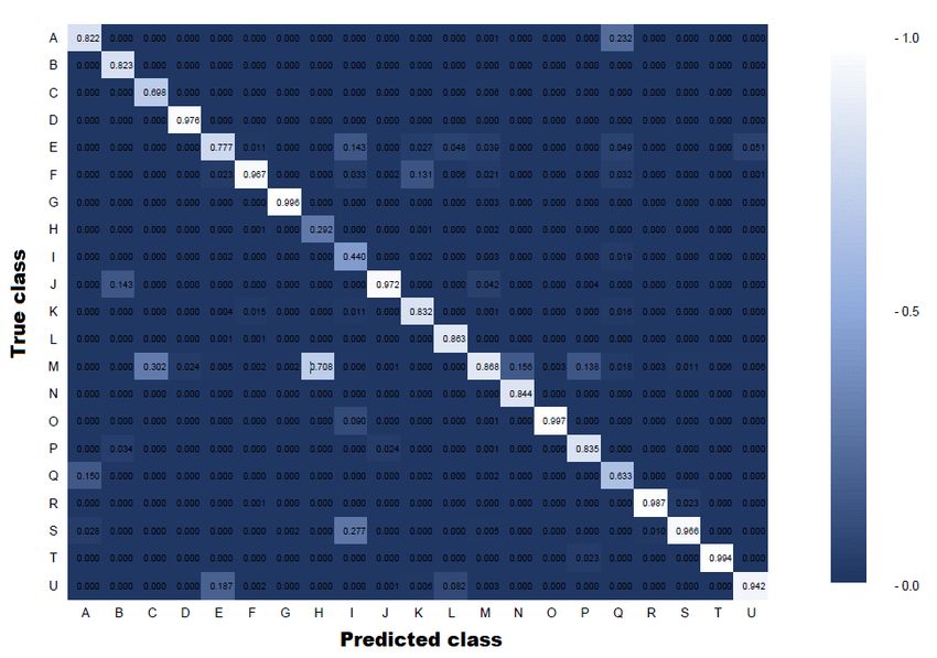
The normalised confusion matrix (Figure 7) demonstrates that
our pipeline is able to identify the majority of the required
classes presented in the panoramic scene. However, we note
classes H (door) and I (desk) are poorly detected.
Figure 4. Results of the hyperparameter’s optimisation process
(Section 4.2).
4.3 Internal dataset
The result of the mIoU evaluation shows that the 70-degree
field of view, a 3:4 aspect ratio, an image size of 840 × 1120
and a spherical subdivision with 32 tangential points is the op-
timal pipeline configuration for this dataset, as shown in Figure
4. It is also remarkable that an increase in the resolution of
the tangential images does not improve the final performance.
Additionally, greater redundancy in the spherical positions also
results in a decreased performance.
The final semantic segmentation image I C with the optimum
hyperparameters is shown in Figure 6 (top). Analysing the
areas captured in the original panorama from the TLS visible
in Figure 5 (top), versus the final segmented image, we note
high precision is achieved at the object boundaries, especially Figure 6. Final semantic segmentation results for our internal
on the furniture and walls. In addition, the mIoU performance dataset (top) and 2D3DS dataset (bottom).
achieved is superior to the analysis of the raw panoramic image
This contribution has been peer-reviewed.
https://doi.org/10.5194/isprs-archives-XLIII-B2-2021-223-2021 | © Author(s) 2021. CC BY 4.0 License. 227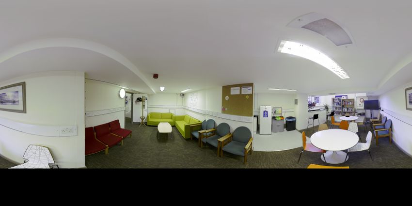
The International Archives of the Photogrammetry, Remote Sensing and Spatial Information Sciences, Volume XLIII-B2-2021
XXIV ISPRS Congress (2021 edition)
CNN, eliminating the need for manually labelled training data
or specialised 3D point cloud networks. This allows us to ex-
ploit large 2D labelled datasets for 3D point cloud semantic
segmentation. Furthermore, our results show that despite our
original data being in an equirectangular projection, we still
achieve reasonable class labels from a network trained on more
commonly available rectilinear images. Whilst we expect res-
ults to improve if a network is trained directly on equirectan-
gular images, we show that this is not strictly necessary. This
significantly reduces workload and accelerates the adoption of
new DL frameworks for TLS data.
ACKNOWLEDGEMENTS
This research was partially funded by the National Agency
for Research and Development (ANID) of the Government of
Chile, through the program ”Magister en el extranjero 2018” -
73190381.
References
Armeni, I., Sax, S., Zamir, A. R., Savarese, S., 2017. Joint
2d-3d-semantic data for indoor scene understanding. arXiv pre-
print arXiv:1702.01105.
Boehm, J., Becker, S., 2007. Automatic marker-free registration
of terrestrial laser scans using reflectance. Proceedings of the
8th conference on optical 3D measurement techniques, Zurich,
Switzerland, 9–12.
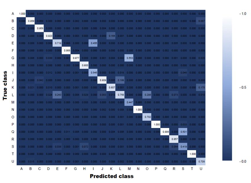
Figure 7. Normalised confusion matrix for our internal dataset Cohen, T. S., Geiger, M., Köhler, J., Welling, M., 2018. Spher-
(top) and 2D3DS dataset (bottom). ical CNNs. International Conference on Learning Representa-
tions.
4.4 2D3DS dataset Demantké, J., Clément Mallet, N. D., Vallet, B., 2011. DIMEN-
SIONALITY BASED SCALE SELECTION IN 3D LIDAR
We processed the selected 2D3DS panorama shown in Figure POINT CLOUDS. International Archives of the Photogram-
5 (bottom), using the same methodology. We obtain the result- metry, Remote Sensing and Spatial Information Sciences,
ing shown in Figure 6 (bottom). The output segmentation map 38(5/W12).
I C is compared to the provided ground truth data. The selected
image has a resolution of 4096 × 2048. The resulting image Eder, M., Shvets, M., Lim, J., Frahm, J. M., 2020. Tangent im-
is generated by considering the best value obtained in the grid ages for mitigating spherical distortion. 2020 IEEE/CVF Con-
search presented before, but adjusting the image size and FOV ference on Computer Vision and Pattern Recognition (CVPR),
resolution, with 80-degrees FOV, an aspect ratio of 3:4, an im- 12423–12431.
age resolution of 600 × 1200 and the spherical interval division
as 32 tangential points. Everingham, M., Van Gool, L., Williams, C. K. I., Winn, J.,
Zisserman, A., 2010. The Pascal Visual Object Classes (VOC)
Qualitatively analysing Figure 6 (bottom vs. top row), it is evid- Challenge. International Journal of Computer Vision, 88(2),
ent that the proposed method does not achieve similar perform- 303–338.
ance in the lower resolution 2D3DS dataset, in comparison with
the internal high-resolution TLS dataset. This is particularly Eysn, L., Pfeifer, N., Ressl, C., Hollaus, M., Grafl, A.,
evident for the ceiling. However quantitatively, it is clear from Morsdorf, F., 2013. A practical approach for extracting tree
the confusion matrix (Figure 7 bottom) that nevertheless most models in forest environments based on equirectangular pro-
areas of the dataset were correctly classified. jections of terrestrial laser scans. Remote Sensing, 5(11), 5424–
5448.
5. CONCLUSION Gonzalez, A., 2009. Measurement of Areas on a Sphere Us-
ing Fibonacci and Latitude–Longitude Lattices. Mathematical
We presented a pipeline for semantic segmentation of TLS Geosciences, 42(1), 49. https://doi.org/10.1007/s11004-009-
point clouds for indoor scenes. We show that by exploiting 9257-x.
co-registered RGB image data, we can perform semantic seg-
mentation using standard 2D CNNs. These labels can then be Griffiths, D., Boehm, J., 2019. A review on deep learning
mapped back onto the original 3D point cloud data. We demon- techniques for 3D sensed data classification. Remote Sensing,
strate satisfactory results using a pre-trained off-the-shelf 2D 11(12), 1499.
This contribution has been peer-reviewed.
https://doi.org/10.5194/isprs-archives-XLIII-B2-2021-223-2021 | © Author(s) 2021. CC BY 4.0 License. 228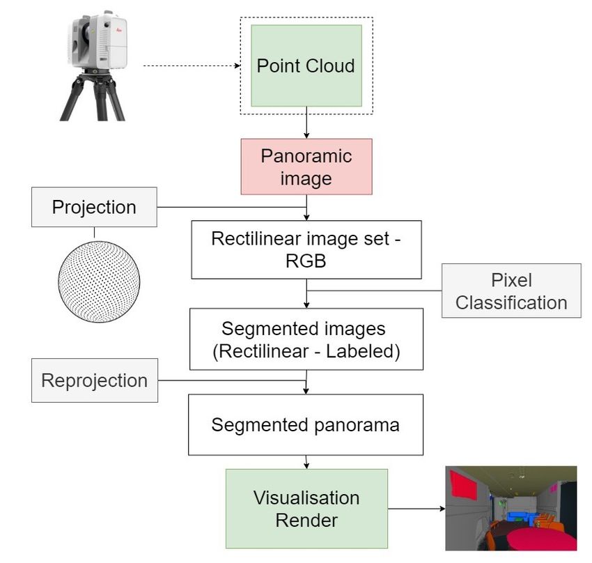
The International Archives of the Photogrammetry, Remote Sensing and Spatial Information Sciences, Volume XLIII-B2-2021
                                                XXIV ISPRS Congress (2021 edition)

Hermosilla, P., Ritschel, T., Vázquez, P.-P., Vinacua, À., Rop-    Xiao, T., Liu, Y., Zhou, B., Jiang, Y., Sun, J., 2018. Unified per-
inski, T., 2018. Monte carlo convolution for learning on non-        ceptual parsing for scene understanding. V. Ferrari, M. Hebert,
uniformly sampled point clouds. ACM Transactions on Graph-           C. Sminchisescu, Y. Weiss (eds), Computer Vision – ECCV
ics (TOG), 37(6), 1–12.                                              2018, Springer International Publishing, Cham, 432–448.

Jiang, C. M., Huang, J., Kashinath, K., Prabhat, Marcus, P.,         Yu, D., Ji, S., 2019. Grid Based Spherical CNN for
Niessner, M., 2019. Spherical CNNs on unstructured grids. In-        Object Detection from Panoramic Images. 19(11), 2622.
ternational Conference on Learning Representations.                  https://www.mdpi.com/1424-8220/19/11/2622.

Liu, K., Boehm, J., 2015. Classification of big point cloud          Zhang, C., Liwicki, S., Smith, W., Cipolla, R., 2019.
data using cloud computing. ISPRS-International Archives of          Orientation-aware semantic segmentation on icosahedron
the Photogrammetry, Remote Sensing and Spatial Information           spheres. 2019 IEEE/CVF International Conference on Com-
Sciences, 40, 553–557.                                               puter Vision (ICCV), 3532–3540.

                                                                     Zhao, Q., Dai, F., Ma, Y., Wan, L., Zhang, J., Zhang, Y., 2018a.
Qi, C. R., Su, H., Mo, K., Guibas, L. J., 2017a. Pointnet: Deep      Spherical superpixel segmentation. IEEE Transactions on Mul-
learning on point sets for 3d classification and segmentation.       timedia, 20(6), 1406–1417.
Proceedings of the IEEE conference on computer vision and
pattern recognition, 652–660.                                        Zhao, Q., Zhu, C., Dai, F., Ma, Y., Jin, G., Zhang, Y., 2018b.
                                                                     Distortion-aware CNNs for spherical images. Proceedings of
Qi, C. R., Yi, L., Su, H., Guibas, L. J., 2017b. Pointnet++: Deep    the 27th International Joint Conference on Artificial Intelli-
hierarchical feature learning on point sets in a metric space.       gence, 1198–1204.
arXiv preprint arXiv:1706.02413.
                                                                     Zhou, B., Zhao, H., Puig, X., Fidler, S., Barriuso, A., Torralba,
Rusu, R. B., Blodow, N., Beetz, M., 2009. Fast point feature         A., 2017. Scene parsing through ade20k dataset. Proceedings
histograms (fpfh) for 3d registration. 2009 IEEE international       of the IEEE conference on computer vision and pattern recog-
conference on robotics and automation, IEEE, 3212–3217.              nition, 633–641.

Salti, S., Tombari, F., Di Stefano, L., 2014. SHOT: Unique sig-
natures of histograms for surface and texture description. Com-
puter Vision and Image Understanding, 125, 251–264.

Tabkha, A., Hajji, R., Billen, R., Poux, F., 2019. Semantic en-
richment of point cloud by automatic extraction and enhance-
ment of 360° panoramas. International Archives of the Photo-
grammetry, Remote Sensing and Spatial Information Sciences,
42(W17), 355–362.

Thomas, H., Qi, C. R., Deschaud, J.-E., Marcotegui, B.,
Goulette, F., Guibas, L. J., 2019. Kpconv: Flexible and de-
formable convolution for point clouds. Proceedings of the
IEEE/CVF International Conference on Computer Vision,
6411–6420.

Wang, Y., Shi, T., Yun, P., Tai, L., Liu, M., 2018. Pointseg:
Real-time semantic segmentation based on 3d lidar point cloud.
arXiv preprint arXiv:1807.06288.

Weinmann, M., Schmidt, A., Mallet, C., Hinz, S., Rottensteiner,
F., Jutzi, B., 2015. Contextual classification of point cloud data
by exploiting individual 3D neigbourhoods. ISPRS Annals of
the Photogrammetry, Remote Sensing and Spatial Information
Sciences II-3 (2015), Nr. W4, 2(W4), 271–278.

Weisstein, E. W., 2018. Gnomonic projection. Publisher:
Wolfram Research, Inc.

Wu, B., Wan, A., Yue, X., Keutzer, K., 2018. Squeezeseg:
Convolutional neural nets with recurrent crf for real-time road-
object segmentation from 3d lidar point cloud. 2018 IEEE In-
ternational Conference on Robotics and Automation (ICRA),
IEEE, 1887–1893.

Wu, W., Qi, Z., Fuxin, L., 2019. Pointconv: Deep con-
volutional networks on 3d point clouds. Proceedings of the
IEEE/CVF Conference on Computer Vision and Pattern Recog-
nition, 9621–9630.

                                                This contribution has been peer-reviewed.
                 https://doi.org/10.5194/isprs-archives-XLIII-B2-2021-223-2021 | © Author(s) 2021. CC BY 4.0 License.               229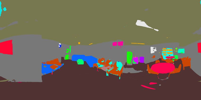
You can also read