SHALLOW WATER BATHYMETRY MAPPING FROM UAV IMAGERY BASED ON MACHINE LEARNING
←
→
Page content transcription
If your browser does not render page correctly, please read the page content below
The International Archives of the Photogrammetry, Remote Sensing and Spatial Information Sciences, Volume XLII-2/W10, 2019
      Underwater 3D Recording and Modelling “A Tool for Modern Applications and CH Recording”, 2–3 May 2019, Limassol, Cyprus

       SHALLOW WATER BATHYMETRY MAPPING FROM UAV IMAGERY BASED ON
                           MACHINE LEARNING

                                           P. Agrafiotis 1,2 ∗, D. Skarlatos 2 , A. Georgopoulos 1 , K. Karantzalos 1
 1
     National Technical University of Athens, School of Rural and Surveying Engineering, Department of Topography, Zografou Campus,
                                             9 Heroon Polytechniou str., 15780, Athens, Greece
                                                   (pagraf, drag, karank)@central.ntua.gr
                2
                  Cyprus University of Technology, Civil Engineering and Geomatics Dept., Lab of Photogrammetric Vision,
                                                 2-8 Saripolou str., 3036, Limassol, Cyprus
                                            (panagiotis.agrafioti, dimitrios.skarlatos)@cut.ac.cy

                                                               Commission II, WG II/9

KEY WORDS: Point Cloud, Bathymetry, SVM, Machine Learning, UAV, Seabed Mapping, Refraction effect

ABSTRACT:

The determination of accurate bathymetric information is a key element for near offshore activities, hydrological studies such as
coastal engineering applications, sedimentary processes, hydrographic surveying as well as archaeological mapping and biological
research. UAV imagery processed with Structure from Motion (SfM) and Multi View Stereo (MVS) techniques can provide
a low-cost alternative to established shallow seabed mapping techniques offering as well the important visual information.
Nevertheless, water refraction poses significant challenges on depth determination. Till now, this problem has been addressed
through customized image-based refraction correction algorithms or by modifying the collinearity equation. In this paper, in order
to overcome the water refraction errors, we employ machine learning tools that are able to learn the systematic underestimation of the
estimated depths. In the proposed approach, based on known depth observations from bathymetric LiDAR surveys, an SVR model
was developed able to estimate more accurately the real depths of point clouds derived from SfM-MVS procedures. Experimental
results over two test sites along with the performed quantitative validation indicated the high potential of the developed approach.

                         1. INTRODUCTION                                      1.1   Description of the problem

Although through-water depth determination from aerial                        Even though UAVs are well established in monitoring and 3D
imagery is a much more time consuming and costly process,                     recording of dry landscapes and urban areas, when it comes
it is still a more efficient operation than ship-borne sounding               to bathymetric applications, errors are introduced due to the
methods and underwater photogrammetric methods (Agrafiotis                    water refraction. Unlike in-water photogrammetric procedures
et al., 2018) in the shallower (less than 10 m depth) clear                   where, according to the literature (Lavest et al., 2000), thorough
water areas. Additionally, a permanent record is obtained of                  calibration is sufficient to correct the effects of refraction, in
other features in the coastal region such as tidal levels, coastal            through-water (two-media) cases, the sea surface undulations
dunes, rock platforms, beach erosion, and vegetation. This is                 due to waves (Fryer and Kniest, 1985, Okamoto, 1982) and
true, even though many alternatives for bathymetry (Menna                     the magnitude of refraction that differ at each point of every
et al., 2018) have arose since. This is especially the case                   image, lead to unstable solutions (Agrafiotis and Georgopoulos,
for the coastal zone of up to 10m depth, which concentrates                   2015, Georgopoulos and Agrafiotis, 2012). More specifically,
most of the financial activities, is prone to accretion or erosion,           according to Snell’s law, the effect of refraction of a light
and is ground for development, where there is no affordable                   beam to water depth is affected by water depth and angle of
and universal solution for seamless underwater and overwater                  incidence of the beam in the air/water interface. The problem
mapping. Image-based techniques fail due to wave breaking                     becomes even more complex when multi view geometry is
effects and water refraction, and echo sounding fails due to                  applied. In Figure 1 the multiple view geometry which applies
short distances.                                                              to the UAV imagery is demonstrated: there, the apparent depth
                                                                              C is calculated by the collinearity equation. Starting from the
At the same time bathymetric LiDAR with simultaneous image                    apparent (erroneous) depth of a point A, its image-coordinates
acquisition is a valid, albeit expensive alternative, especially              a1 , a2 , a3 . . . , an , can be backtracked in images O1 , O2 , O3 ,
for small scale surveys. In addition, despite the fact that the               . . . , On using the standard collinearity equation. If a point has
image acquisition for orthophotomosaic generation in land is a                been matched successfully in the photos O1 , O2 , O3 , . . . , On ,
solid solution, the same cannot be said for the shallow water                 then the standard collinearity intersection would have returned
seabed. Despite the accurate and precise depth map provided                   the point C, which is the apparent and shallower position of
by LiDAR, the sea bed orthoimage generation is prohibited due                 point A and in the multiple view case is the adjusted position of
to the refraction effect, leading to another missed opportunity               all the possible red dots in Figure 1, which are the intersections
to benefit from a unified seamless mapping process.                           for each stereopair. Thus, without some form of correction,
                                                                              refraction produce an image and consequently a point cloud
                                                                              of the submerged surface which appears to lie at a shallower
     ∗ Corresponding   author, email: pagraf@central.ntua.gr                  depth than the real surface. In literature, two main approaches

                                                     This contribution has been peer-reviewed.
                         https://doi.org/10.5194/isprs-archives-XLII-2-W10-9-2019 | © Authors 2019. CC BY 4.0 License.                           9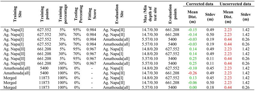
The International Archives of the Photogrammetry, Remote Sensing and Spatial Information Sciences, Volume XLII-2/W10, 2019
       Underwater 3D Recording and Modelling “A Tool for Modern Applications and CH Recording”, 2–3 May 2019, Limassol, Cyprus

                                                                     1.3   Bathymetry Determination using Machine Learning

                                                                     Even though the presented approach here is the only one
                                                                     dealing with UAV imagery and dense point clouds resulting
                                                                     from the SfM-MVS processing, there is a small number of
                                                                     single image approaches for bathymetry retrieval using satellite
                                                                     imagery. Most of these methods are based on the relation
                                                                     between the reflectance and the depth. These approaches
                                                                     exploit a support vector machine (SVM) system to predict
                                                                     the correct depth (Wang et al., 2018, Misra et al., 2018).
                                                                     Experiments there showed that the localized model reduced the
                                                                     bathymetry estimation error by 60% from an RMSE of 1.23m to
                                                                     0.48m. In (Mohamed et al., 2016) a methodology is introduced
                                                                     using an Ensemble Learning (EL) fitting algorithm of Least
                                                                     Squares Boosting (LSB) for bathymetric maps calculation in
                                                                     shallow lakes from high resolution satellite images and water
                                                                     depth measurement samples using Echo-sounder. The retrieved
                                                                     bathymetric information from the three methods was evaluated
                                                                     using Echo Sounder data. The LSB fitting ensemble resulted
 Figure 1. The geometry of two-media photogrammetry for the          in an RMSE of 0.15m where the PCA and GLM yielded
                     multiple view case                              RMSE’s of 0.19m and 0.18m respectively over shallow water
                                                                     depths less than 2m. Except from the primary data used, the
to correct refraction in through-water photogrammetry can be         main difference between the work presented here and the work
found; analytical or image based.                                    presented in these articles, is that they test and evaluate their
                                                                     proposed algorithms on percentages of the same test site and at
In this work, a new approach to address the systematic               very shallow depths while here two different test sites are used.
refraction errors of point clouds derived from SfM-MVS
procedures is introduced. The developed technique is based
on machine learning tools which are able to accurately recover                               2. DATASETS
shallow bathymetric information from UAV-based imaging
datasets, leveraging several coastal engineering applications.       The proposed methodology has been applied in real-world
In particular, the goal was to deliver image-based point             applications in two different test sites for verification and
clouds with accurate depth information by learning to estimate       comparison against bathymetric LiDAR data. In the following
the correct depth from the systematic differences between            paragraphs, the results of the proposed methodology are
image-based products and (the current gold-standard for              investigated and evaluated. The initial point cloud used here can
shallow waters) LiDAR point clouds. To this end, a Linear            be created by any commercial photogrammetric software (such
Support Vector Regression model was employed and trained             as Agisoft’s Photoscan c , used in this study) following standard
to predict the actual depth Z from the apparent depth of a           process, without water refraction compensation. However,
point, Zo from the image-based point cloud. The rest of the          wind affects the sea surface with wrinkles and waves. Taking
paper is organized as follows: Subsection 1.2 presents the           this into account, the water surface needs to be as flat as
related work regarding refraction correction and the use of          possible, so that to have best sea bottom visibility and follow the
SVMs in bathymetry determination. In Section 2, datasets used        assumption of flat-water surface. In case of a wavy sea surface,
are described while in Section 3 the proposed methodology is         errors would be introduced (Okamoto, 1982, Agrafiotis and
described and justified. In Section 4 the tests performed and the    Georgopoulos, 2015) without any form of correction (Chirayath
evaluations carried out are described. Section 5 concludes the       and Earle, 2016) applied and the relation of the real and the
paper.                                                               apparent depths will be more scattered, affecting to some extent
                                                                     the training and the fitting of the model. Furthermore, water
1.2     Related work                                                 should not be turbid enough to have a clear bottom view.
                                                                     Obviously, water turbidity and water visibility are additional
Refraction effect has driven scholars to suggest several models      restraining factors. Just like in any photogrammetric project,
for two-media photogrammetry, most of which are dedicated            sea bottom must present pattern, meaning that photogrammetric
to specific applications.      Two-media photogrammetry is           bathymetry might fail in sandy or seagrass sea bed. However,
divided into through-water and in-water photogrammetry. The          since normally, a sandy bottom does not present any abrupt
through-water term is used when the camera is above the water        height differences and detailed forms, and provided measures to
surface and the object is underwater, hence part of the ray          eliminate the noise of the point cloud in these areas are taken,
is traveling through air and part of it through water. It is         results would be acceptable, even in a less dense point cloud,
most commonly used in aerial photogrammetry (Skarlatos and           due to matching difficulties.
Agrafiotis, 2018, Dietrich, 2017) or in close range applications
(Georgopoulos and Agrafiotis, 2012, Butler et al., 2002).            2.1   Test sites and available data
It is argued that if the water depth to flight height ratio
is considerably low, then water refraction is unnecessary.           In order to facilitate the training and the testing of the proposed
However, as shown in the literature (Skarlatos and Agrafiotis,       approach, ground truth data of the seabed depth were required,
2018), the water depth to flying height ratio is irrelevant, in      together with the image-based point clouds. To facilitate this,
cases ranging from drone and unmanned aerial vehicle (UAV)           ground control points (GCPs) were measured in land and used
mapping to full-scale manned aerial mapping. In these cases          to georeference the photogrammetric data with the LiDAR data.
water refraction correction is necessary.                            The common system used is the Cyprus Geodetic Reference

                                                 This contribution has been peer-reviewed.
                     https://doi.org/10.5194/isprs-archives-XLII-2-W10-9-2019 | © Authors 2019. CC BY 4.0 License.                   10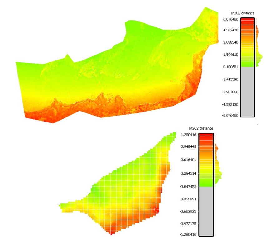
The International Archives of the Photogrammetry, Remote Sensing and Spatial Information Sciences, Volume XLII-2/W10, 2019
    Underwater 3D Recording and Modelling “A Tool for Modern Applications and CH Recording”, 2–3 May 2019, Limassol, Cyprus

System (CGRS) 1993, to which the LiDAR data were already             points having Zo ≥ Z since this is not valid when the refraction
georeferenced.                                                       phenomenon is present. Moreover, points having Zo ≥ 0m
                                                                     were also removed since they might cause errors in the training
2.1.1 Amathouda Test Site The first site used is                     process. After being pre-processed, the datasets were used as
Amathouda (Figure 2 upper image), where the seabed                   follows: due to availability of a lot of reference data in Agia
reaches a maximum depth of 5.57 m. The flight was executed           Napa test site, the site was split in two parts having different
with a Swinglet CAM fixed-wing UAV with an Canon IXUS                characteristics: Part I having 627.522 points (Figure 3(left)
220HS camera having 4.3mm focal length, 1.55µm pixel size            in the red rectangle on the left, Figure 5(top left)) and Part
and 4000×3000 pixels format. A total of 182 photos were              II having 661.208 points (Figure 3(left) in the red rectangle
acquired, from an average flight height of 103 m, resulting in       on the right, Figure 5(top right)). Amathouda dataset (Figure
3.3 cm average GSD.                                                  3(middle) and Figure 5(bottom left)) was not split since the
                                                                     available points were much less and quite scattered (Figure
2.1.2 Agia Napa Test Site The second test site is in Agia            3(right)). The distribution of the Z and Zo of the points is
Napa (Figure 2 lower image), where the seabed reaches the            presented in Figure 3(right) the Agia Napa dataset is presented
depth of 14.8m. The flight here executed with the same UAV.          with blue colour, while the Amathouda dataset is presented with
In total 383 images were acquired, from an average flight            orange colour.
height of 209m, resulting in 6.3cm average ground pixel size.
Table 1(presents the flight and image-based processing details       2.1.4 LiDAR Reference data LiDAR point clouds of the
                                                                     submerged areas were used as reference data for training
                                                                     and evaluation of the developed methodology. These point
                                                                     clouds were generated with the RIEGL LMS Q680i (RIEGL
                                                                     Laser Measurement Systems GmbH, 3580 Horn, Austria), an
                                                                     airborne LiDAR system. This instrument uses the time-of-flight
                                                                     distance measurement principle of infrared nanosecond pulses
                                                                     for topographic applications and of green (532nm) nanosecond
                                                                     pulses for bathymetric applications. Table 3 presents the
                                                                     details of the LiDAR data used.      Even though the specific
  Figure 2. The two test sites. Amathouda (top) and Ag. Napa
    (bottom). Yellow triangles represent the GCPs positions.

of the two different test sites. There, it can be noticed that the
two sites have a different average flight height, indicating that
the suggested solution is not limited to specific flight heights.
That means that a trained model on an area may be applied                          Table 2. LiDAR data specifications
on another area, having the flight and image-based processing
characteristics of the datasets used.
                                                                     LiDAR system can offer point clouds with accuracy of 20mm
                                                                     in topographic applications according to the manufacturers,
                                                                     when it comes to bathymetric applications the system’s range
                                                                     error range is in the order of +/-50-100mm for depths up to
                                                                     4m, similar to other conventional topographic airborne scanners
                                                                     (Steinbacher et al., 2012). According to the literature LiDAR
                                                                     bathymetry data can be affected by significant systematic errors
                                                                     that lead to much greater errors. In (Skinner, 2011) the average
                                                                     error in elevations for the wetted river channel surface area
                                                                     was -0.5% and ranged from -12% to 13%. In (Bailly et
                                                                     al., 2010) authors detected a random error of 0.19m-0.32m
                                                                     for the riverbed elevation from the Hawkeye II sensor. In
                                                                     (Fernandez-Diaz et al., 2014) the standard deviation of the
Table 1. Flight and image-based processing details regarding the     bathymetry elevation differences calculated reaches 0.79m,
                     two different test sites                        with 50% of the differences falling between 0.33m to 0.56m.
                                                                     However, according to the authors it appears that most of these
                                                                     differences are due to sediment transport between observation
                                                                     epochs. In (Westfeld et al., 2017) authors report that the RMSE
2.1.3 Data pre-processing To facilitate the training of              of the lateral coordinate displacement is 2.5% of the water
the proposed bathymetry correction model, data were                  depth for the smooth, rippled sea swell. Assuming a mean
pre-processed. Since the image-based point cloud was denser,         water depth of 5m leads to a RMSE of 12cm. If a light sea
than the LiDAR point cloud, it was decided to reduce the             state with small wavelets assumed, results with an RMSE of
number of the points of the first one. To that direction the         3.8% which corresponds to 19cm in 5m water are expected.
number of the image-based point clouds were reduced to the           It becomes obvious that wave patterns can cause significant
number of the LiDAR point clouds, for the two test sites.            systematic effects in bottom coordinate locations. Even for very
This way, for each position X, Y of the seabed two depths are        calm sea states, the lateral displacement can be up to 30cm at
corresponding: the apparent depth Zo and the LiDAR depth             5m water depth (Westfeld et al., 2017).
Z. Consequently, outlier data were removed from the dataset.
At this stage of the pre-processing, outliers were considered        Considering the above, authors would like to highlight here that

                                                This contribution has been peer-reviewed.
                    https://doi.org/10.5194/isprs-archives-XLII-2-W10-9-2019 | © Authors 2019. CC BY 4.0 License.                 11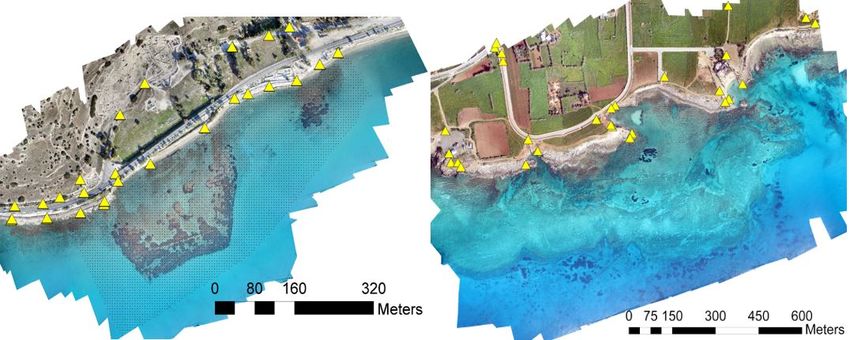
The International Archives of the Photogrammetry, Remote Sensing and Spatial Information Sciences, Volume XLII-2/W10, 2019
    Underwater 3D Recording and Modelling “A Tool for Modern Applications and CH Recording”, 2–3 May 2019, Limassol, Cyprus

Figure 3. The two test areas from the Agia Napa test site are presented (left) with blue colour: Part I on the left and Part II on the right.
  The Amathouda test site is presented in the middle with orange colour. The distribution of the Z and Zo values for each dataset is
                                                       presented (right) as well.

in the proposed approach, LiDAR point clouds are used for               the SVM Linear Regression and they were highly dependent on
training the suggested model, since this is the State-of-the-Art        the training dataset and its density, being very sensitive to the
method used for shallow water bathymetry of large areas                 noise of the point cloud. This is explained by the fact that the
(Menna et al., 2018), even though in some cases the absolute            two regression methods differ only in the loss function where
accuracy of the resulting point clouds is deteriorated. These           SVM minimizes hinge loss while logistic regression minimizes
issues do not affect the principle of the main goal of the              logistic loss and logistic loss diverges faster than hinge loss
presented approach which is to systematically solve the depth           being more sensitive to outliers. This is apparent also in Figure
underestimation problem, by predicting the correct depth, as            4, where the predicted models using a simple Linear Regression
proved in the next sections.                                            and an SVM Linear Regression trained on Amathouda and
                                                                        Agia Napa [I] datasets are plotted. In the case of training on
                                                                        the Amathouda dataset, it is obvious that the two predicted
             3. PROPOSED METHODOLOGY
                                                                        models (lines in red and cyan colour) differ considerably as
A Support Vector Regression (SVR) method is adopted in                  the depth increases, leading to different depth predictions.
order to address the described problem. To that direction, data         However, in the case of the models trained in Agia Napa [I]
available from two different test sites, characterized by different     dataset, the two predicted models (lines in magenta and yellow
type of seabed and depths are used to train, validate and test          colour) are overlapping, also with the predicted model of the
the proposed approach. The Linear SVR model was selected                SVM Linear Regression, trained on Amathouda. These results
after studying the relation of the real (Z) and the apparent            suggest that the SVM Linear Regression is less dependent
(Zo ) depths of the available points (Figure 3(right)). Based on        on the density and the noise of the data and ultimately the
the above, the SVR model fits according to the given training           more robust method, predicting systematically reliable models,
data: the LiDAR (Z) and the apparent depths (Zo ) of many               outperforming simple Linear Regression.
3D points. After fitting, the real depth can be predicted in
                                                                        3.1    Linear SVR
the cases where only the apparent depth is available. In the
performed study the relationship of the LiDAR (Z) and the
                                                                        SVMs can also be applied to regression problems by the
apparent depths (Zo ) of the available points rather follows a
                                                                        introduction of an alternative loss function (Smola et al., 1996).
linear model and as such, a deeper learning architecture was not
                                                                        The loss function must be modified to include a distance
considered necessary. The use of a simple Linear Regression
                                                                        measure. In this paper, a Linear Support Vector Regression
                                                                        model is used exploiting the implementation of (Pedregosa et
                                                                        al., 2011). The problem is formulated as follows: consider the
                                                                        problem of approximating the set of depths:

                                                                           D = {(Z01 , Z 1 ), ..., (Z0l , Z l )},   Z0 ∈ R n ,   Z ∈ R (1)

                                                                        with a linear function

                                                                                                  f (Z0 ) = hw, Z0 i + b                 (2)

                                                                        The optimal regression function is given by the minimum of the
                                                                        functional,

Figure 4. The established correlations based on a simple Linear                                        1          X −
                                                                                       φ(w, Z0 ) =       kwk2 + c  (ξi + ξi+ )           (3)
  Regression and SVM Linear Regression models, trained on                                              2
                                                                                                                     i
             Amathouda and Agia Napa datasets.
                                                                        Where c is a pre-specified positive numeric value that controls
model was also examined, fitting tests were performed in the            the penalty imposed on observations that lie outside the epsilon
two test sites and predicted values were compared to the LiDAR          margin (ε) and helps to prevent overfitting (regularization).
data. However, this approach was rejected since the predicted           This value determines the trade-off between the flatness of
models were producing larger errors than the ones produced by           f (Zo ) and the amount up to which deviations larger than ε are

                                                This contribution has been peer-reviewed.
                    https://doi.org/10.5194/isprs-archives-XLII-2-W10-9-2019 | © Authors 2019. CC BY 4.0 License.                         12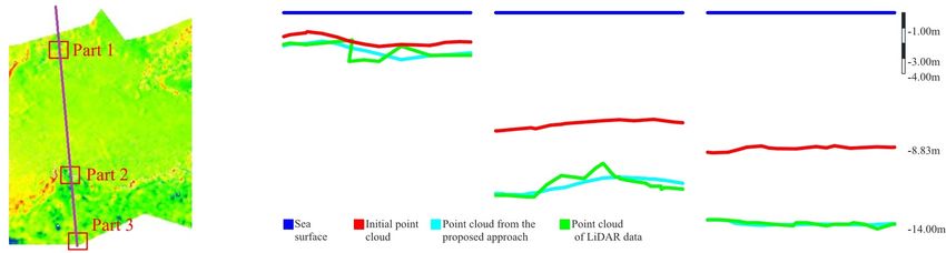
The International Archives of the Photogrammetry, Remote Sensing and Spatial Information Sciences, Volume XLII-2/W10, 2019
       Underwater 3D Recording and Modelling “A Tool for Modern Applications and CH Recording”, 2–3 May 2019, Limassol, Cyprus

                                                                     Z-Zo distribution of this “merged dataset” is presented in Figure
                                                                     5(bottom right). In the same figure the Z-Zo distribution of
                                                                     the Agia Napa dataset and Amathouda dataset are presented in
                                                                     blue and yellow colour respectively. This dataset was generated
                                                                     using the total of the Amathouda dataset points and 1% of the
                                                                     Agia Napa Part II dataset.

                                                                     4.2   Evaluation of the results

                                                                     Figure 6 demonstrates four of the predicted models: the black
                                                                     coloured line represents the predicted model trained on the
                                                                     Merged Dataset, the cyan coloured line represents the predicted
                                                                     model trained on the Amathouda Dataset, the red coloured
                                                                     line represents the predicted model trained on the Agia Napa
                                                                     Part I [30%] Dataset, and the green coloured line represents
                                                                     the predicted model trained on the Agia Napa Part II [30%]
                                                                     Dataset. It is obvious that despite the scattered points which

  Figure 5. The Z-Zo distribution of the used datasets: the Agia
  Napa Part I dataset over the full Agia Napa dataset (top left),
  The Agia Napa Part II dataset over the full Agia Napa dataset
(top right), Amathouda dataset (bottom left), The merged dataset
   over the Agia Napa and Amathouda datasets (bottom right).

tolerated, and ξi −, ξi + are slack variables representing upper
and lower constraints of the outputs of the system, Z is the
real depth of a point X, Y and Zo is the apparent depth of the
same point X, Y. Based on the above, the proposed framework          Figure 6. The Z-Zo distribution of the employed datasets and the
is trained using the real (Z) and the apparent (Zo ) depths of a                    respective predicted linear models
number of points in order to predict the real depth in the cases
where only the apparent depth is available.                          lie away from these lines, the models achieve to follow the
                                                                     Z-Zo distribution of most of the points. It is important to
                4. TESTS AND EVALUATION                              highlight here that the differences between the predicted model
                                                                     trained on the Amathouda dataset (cyan line) and the predicted
4.1     Training, Validation and Testing                             models trained on Agia Napa datasets are not remarkable, even
                                                                     though the maximum depth of Amathouda dataset is 5.57m
In order to evaluate the performance of the developed model          and the maximum depth of Agia Napa datasets is 14.8m and
in terms of robustness and effectiveness, six different training     14.7m respectively. The biggest difference observed between
sets were formed from two test sites of different seabed             the predicted models is between the predicted model trained
characteristics and then validated against 13 different testing      on Agia Napa [II] dataset (green line) and the predicted model
sets.                                                                trained on the Merge dataset (black line): 0.45m at 16.8m
                                                                     depth, or a 2.7% of the real depth. In the next paragraphs the
4.1.1 Agia Napa and Amathouda datasets The first and                 results of the proposed method are evaluated in terms of cloud
the second training approaches are using 5% and 30% of the           to cloud distances. Additionally, cross sections of the seabed
Agia Napa Part II dataset respectively in order to fit the Linear    are presented to highlight the high performance of the proposed
SVR model and predict the correct depth over the Agia Napa           methodology and the issues and differences observed between
Part I and Amathouda test sites. The third and the fourth            the tested and ground truth point clouds.
training approaches are using 5% and 30% of the Agia Napa
Part I dataset respectively in order to fit the Linear SVR model     4.2.1 Multiscale Model to Model Cloud Comparison To
and predict the correct depth over the Agia Napa Part II and         evaluate the results of the proposed methodology, the initial
Amathouda test sites. The fifth training approach is using 100%      point clouds of the SfM-MVS procedure and the point clouds
of the Amathouda dataset in order to fit the Linear SVR model        resulted from the proposed methodology were compared with
and predict the correct depth over the Agia Napa Part I, the Agia    the LiDAR point cloud using the Multiscale Model to Model
Napa Part II and their combination. The Z-Zo distribution of         Cloud Comparison (M3C2) (Lague et al., 2013) in Cloud
the points used for this training can be seen in Figure 5(bottom     Compare freeware (Cloud Compare, 2019) to demonstrate the
left). It is important to notice here that the maximum depth of      changes and the differences that are applied by the presented
the training dataset is 5.57m while the maximum depth of the         depth correction approach. The M3C2 algorithm offers
testing datasets is 14.8m and 14.7m respectively.                    accurate surface change measurement that is independent of
                                                                     point density (Lague et al., 2013). In Figure 7(top) and
4.1.2 Merged dataset Finally, a sixth training approach is           Figure 7(bottom), the distances between the reference data
performed by creating a virtual dataset containing almost the        and the original image-based point clouds are increasing as
same number of points from each of these two datasets. The           the depth increases. These comparisons make clear that the

                                                 This contribution has been peer-reviewed.
                     https://doi.org/10.5194/isprs-archives-XLII-2-W10-9-2019 | © Authors 2019. CC BY 4.0 License.                 13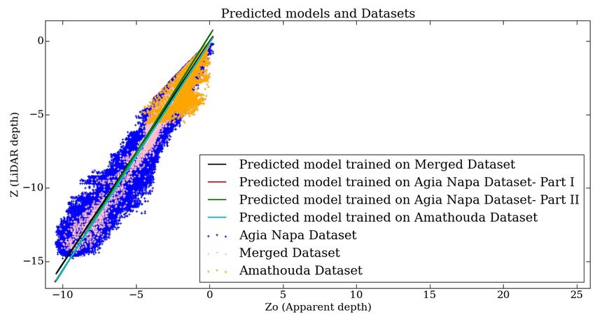
The International Archives of the Photogrammetry, Remote Sensing and Spatial Information Sciences, Volume XLII-2/W10, 2019
Underwater 3D Recording and Modelling “A Tool for Modern Applications and CH Recording”, 2–3 May 2019, Limassol, Cyprus
refraction effect cannot be ignored in such applications. In a totally different and shallower test site. Additionally, areas
both cases demonstrated in Figure 7(top) and Figure 7(bottom), with small rock formations are also presenting large differences.
the Gaussian mean of the differences is significant reaching This is attributed to the different level of detail in these areas
0.44 m (RMSE 0.51m) in the Amathouda test site and 2.23m between the LiDAR point cloud and the image-based one, since
(RMSE 2.64m) in the Agia Napa test site. Since these values LiDAR average point spacing is about 1.1m. These small rock
might be considered ‘negligible’ in some applications, it is formations in many cases lead M3C2 to detect larger distances
important to stress that in the Amathouda test site more than in these parts of the site and are responsible for the increased
30% of the compared image-based points present a difference Standard Deviation of the M3C2 distances (Table 3).
of 0.60-1.00m from the LiDAR points, while in Agia Napa,
the same percentage presents differences of 3.00-6.07m, i.e. 4.2.2 Seabed cross sections Several differences observed
20% - 41.1% percent of the real depth. Figure 8 presents the between the image-based point clouds and the LiDAR data that
are not due to the proposed depth correction approach. Cross
sections of the seabed were generated with main aim to prove
the performance of the proposed method, excluding differences
between the compared point clouds. In Figure 9 the footprint
of a representative cross section is demonstrated together with
three parts of the section. These parts highlight the high
performance of the algorithm and the differences between the
point clouds, reported above. In more detail, in the first and the
second part of the section presented, it can be noticed that even
if the corrected image-based point cloud is almost matching
the LiDAR one on the left and the right side of the sections,
in the middle parts, errors are introduced. These are mainly
caused by coarse errors which though are not related to the
depth correction approach. However, in the third part of the
section, it is obvious that even when the depth reaches 14m,
the corrected image-based point cloud matches the LiDAR one,
indicating a very high performance of the proposed approach.
Excluding these differences, the corrected image-based point
cloud presents deviations of less than 0.05m (0.36% remaining
error at 14m depth) from the LiDAR point cloud.
Figure 7. The initial M3C2 distances between the (reference) 4.2.3 Fitting Score Another measure to evaluate the
LiDAR point cloud and the image-based point clouds derived predicted model in cases where a percentage of the dataset has
from the SfM-MVS. Figure 7(top) presents the M3C2 distances been used for training and the rest percentage has been used for
of Agia Napa and Figure 7(bottom) the initial distances for testing is by computing the coefficient R2 which is the fitting
Amathouda test site. score and is defined as
(Ztrue − Zpredicted )2
P
cloud to cloud distances (M3C2) between the LiDAR point R2 = 1 − P (4)
(Ztrue − Ztrue.mean )2
cloud and the point clouds resulted from the predicted model
trained on each dataset. Table 3 presents the results of each
The best possible score is 1.0 and it can also be negative
one of the 13 tests performed with every detail. There, a
(Pedregosa et al., 2011). Ztrue is the real value of the depth
great improvement is observed. More specifically, in Agia
of the points not used for training while the Zpredicted is the
Napa [I] test site, the initial 2.23m mean distance is reduced
predicted depth for these points, using the model trained on
to -0.10m while in Amathouda, the initial mean distance of
the rest of the points. The fitting score is calculated only in
0.44m is reduced to -0.03m, including outlier points such as
cases where a percentage of the dataset is used for training.
seagrass that are not captured in the LiDAR point clouds for
Results in Table 3 highlight the robustness of the proposed
both cases or are caused due to point cloud noise again in
depth correction framework.
areas with seagrass or poor texture. It is important also to
note that the large distances between the clouds observed in
Figure 7 disappear. This improvement is observed in every 5. CONCLUSIONS
test performed proving that the proposed methodology based
on Machine Learning achieves great reduction of the errors In the proposed approach, based on known depth observations
caused by the refraction in the seabed point clouds. In Figure from bathymetric LiDAR surveys, an SVR model was
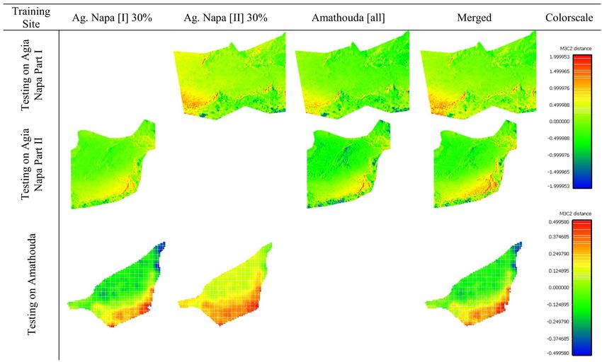
8, it is obvious that the larger differences between the predicted developed able to estimate with high accuracy the real depths of
and the LiDAR depths are observed in some specific areas, or point clouds derived from conventional SfM-MVS procedures.
areas with same characteristics. In more detail, the lower-left Experimental results over two test sites along with the
area of Agia Napa Part I test site and the lower-right area of performed quantitative validation indicated the high potential
Agia Napa Part II test site, have constantly larger error than of the developed approach and the wide field for machine and
other areas of the same depth. This can be explained by their deep learning architectures in bathymetric applications. It is
position in the photogrammetric block, since these are areas proved that the model can be trained on one area and used
far for from the control points, situated in the shore and they on another one, or indeed on many other, having different
are in the outer area of the block. However, it is noticeable characteristics and achieving results of very high accuracy. The
that these two areas, present smaller deviation from the LiDAR proposed approach can be used also in areas were LiDAR data
point cloud, when the model is trained in Amathouda test site, of low density are available, in order to create a denser seabed
This contribution has been peer-reviewed.
https://doi.org/10.5194/isprs-archives-XLII-2-W10-9-2019 | © Authors 2019. CC BY 4.0 License. 14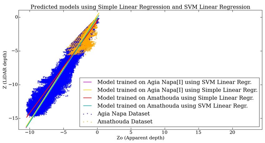
The International Archives of the Photogrammetry, Remote Sensing and Spatial Information Sciences, Volume XLII-2/W10, 2019
    Underwater 3D Recording and Modelling “A Tool for Modern Applications and CH Recording”, 2–3 May 2019, Limassol, Cyprus

                  Table 3. The results of the comparisons between the predicted models for all the tests performed.

Figure 8. The cloud to cloud (M3C2) distances between the LiDAR point cloud and the recovered point clouds after the application of
the proposed approach. The first, the second and the third row of the figure demonstrate the calculated distance maps and their colour
                          scales for the Agia Napa (Part I and Part II) and Amathouda test sites respectively

Figure 9. Indicative cross-sections (X and Y axis having the same scale) from the Agia Napa (Part I) region after the application of the
  proposed approach when trained with 30% from the Part II region. The blue line corresponds to water surface while the green one
  corresponds to LiDAR data. The cyan line is the recovered depth after the application of the proposed approach, while the red line
                        corresponds to the depths derived from the initial uncorrected image-based point cloud.

                                                This contribution has been peer-reviewed.
                    https://doi.org/10.5194/isprs-archives-XLII-2-W10-9-2019 | © Authors 2019. CC BY 4.0 License.                    15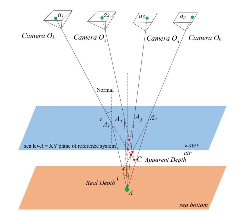
The International Archives of the Photogrammetry, Remote Sensing and Spatial Information Sciences, Volume XLII-2/W10, 2019
    Underwater 3D Recording and Modelling “A Tool for Modern Applications and CH Recording”, 2–3 May 2019, Limassol, Cyprus

representation. The methodology is independent from the UAV         Fryer, J.G., Kniest, H.T., 1985. Errors in depth determination
system used, also the camera and the flight height and there        caused by waves in through-water photogrammetry. The
is no need for additional data i.e. camera orientations, camera     Photogrammetric Record, 11, 745–753.
intrinsic etc. for predicting the correct depth of a point cloud.   Georgopoulos, A., Agrafiotis, P., 2012. Documentation of a
This is a very important asset of the proposed method in relation   submerged monument using improved two media techniques.
to the other state of the art methods used for overcoming           2012 18th International Conference on Virtual Systems and
refraction errors in seabed mapping. The limitations of this        Multimedia, 173–180.
method are mainly imposed by the SfM-MVS errors in areas
having texture of low quality (e.g. sand and seagrass areas).       Guenther, G.C., Cunningham, A.G., LaRocque, P.E., Reid,
                                                                    D.J., 2000. Meeting the accuracy challenge in airborne
Limitations are also imposed due to incompatibilities between       bathymetry. Technical report, NATIONAL OCEANIC
the LiDAR point cloud and the image-based one. Among                ATMOSPHERIC ADMINISTRATION/NESDIS SILVER
ohers, the different level of detail imposed additional errors      SPRING MD.
in the point cloud comparison and compromise the absolute
accuracy of the method. However, twelve out of thirteen             Lague, D., Brodu, N., Leroux, J., 2013. Accurate 3D
                                                                    comparison of complex topography with terrestrial laser
different tests (Table 3) proved that the proposed method           scanner: Application to the Rangitikei canyon (NZ). ISPRS
meets and exceeds the accuracy standards generally accepted         journal of photogrammetry and remote sensing, 82, 10–26.
for hydrography established by the International Hydrographic
Organization (IHO), where in its simplest form, the vertical        Lavest, J.M., Rives, G., Lapresté, J.T., 2000. Underwater
accuracy requirement for shallow water hydrography can be set       camera calibration. European Conference on Computer Vision,
                                                                    Springer, 654–668.
as a total of ±25cm (one sigma) from all sources, including
tides (Guenther et al., 2000).                                      Menna, F., Agrafiotis, P., Georgopoulos, A., 2018. State of the
                                                                    art and applications in archaeological underwater 3D recording
                                                                    and mapping. Journal of Cultural Heritage, 33, 231 - 248.
                 ACKNOWLEDGEMENTS
                                                                    Misra, A., Vojinovic, Z., Ramakrishnan, B., Luijendijk,
Authors would like to acknowledge the Dep. of Land and              A., Ranasinghe, R., 2018. Shallow water bathymetry
Surveys of Cyprus for providing the LiDAR reference data, and       mapping using Support Vector Machine (SVM) technique and
                                                                    multispectral imagery. International journal of remote sensing,
the Cyprus Dep. of Antiquities for permitting the flight over the   39, 4431–4450.
Amathouda site and commissioning the flight over Ag. Napa.
Also, authors would like to thank Dr. Ioannis Papadakis for the     Mohamed, H., Negm, A.m, Zahran, M., Saavedra, O.C.,
discussions on the physics of the refraction effect.                2016. Bathymetry determination from high resolution satellite
                                                                    imagery using ensemble learning algorithms in Shallow
                                                                    Lakes: case study El-Burullus Lake. International Journal of
                       REFERENCES                                   Environmental Science and Development, 7, 295.

Agrafiotis, P., Georgopoulos, A., 2015. CAMERA                      Okamoto, A., 1982. Wave influences in two-media
CONSTANT IN THE CASE OF TWO MEDIA                                   photogrammetry. Photogrammetric Engineering and Remote
PHOTOGRAMMETRY. ISPRS - International Archives of                   Sensing, 48, 1487–1499.
the Photogrammetry, Remote Sensing and Spatial Information
Sciences, XL-5/W5, 1–6.                                             Pedregosa, F., Varoquaux, G., Gramfort, A., Michel, V.,
                                                                    Thirion, B., Grisel, O., Blondel, M., Prettenhofer, P., Weiss,
Agrafiotis, P., Skarlatos, D., Forbes, T., Poullis, C.,             R., Dubourg, V. et al., 2011. Scikit-learn: Machine learning in
Skamantzari, M., Georgopoulos, A., 2018. UNDERWATER                 Python. Journal of machine learning research, 12, 2825–2830.
PHOTOGRAMMETRY IN VERY SHALLOW WATERS:
MAIN CHALLENGES AND CAUSTICS EFFECT                                 Skarlatos, D., Agrafiotis, P., 2018. A Novel Iterative Water
REMOVAL. ISPRS - International Archives of the                      Refraction Correction Algorithm for Use in Structure from
Photogrammetry, Remote Sensing and Spatial Information              Motion Photogrammetric Pipeline. Journal of Marine Science
Sciences, XLII-2, 15–22.                                            and Engineering, 6, 77.

Bailly, J.S., Le Coarer, Y., Languille, P., Stigermark, C.J.,       Skinner, K.D., 2011. Evaluation of lidar-acquired bathymetric
Allouis, T., 2010. Geostatistical estimations of bathymetric        and topographic data accuracy in various hydrogeomorphic
LiDAR errors on rivers. Earth Surface Processes and                 settings in the deadwood and south fork boise rivers,
Landforms, 35, 1199–1210.                                           west-central idaho, 2007. Technical report.
Butler, J., Lane, S., Chandler, J., Porfiri, E., 2002.              Smola, A.J. et al., 1996. Regression estimation with support
Through-water close range digital photogrammetry in flume           vector learning machines. PhD thesis, Master’s thesis,
and field environments. The Photogrammetric Record, 17,             Technische Universität München.
419–439.
                                                                    Steinbacher, F., Pfennigbauer, M., Aufleger, M., Ullrich,
Chirayath, V., Earle, S.A., 2016. Drones that see through           A., 2012. High resolution airborne shallow water mapping.
waves–preliminary results from airborne fluid lensing for           International Archives of the Photogrammetry, Remote Sensing
centimetre-scale aquatic conservation. Aquatic Conservation:        and Spatial Information Sciences, Proceedings of the XXII
Marine and Freshwater Ecosystems, 26, 237–250.                      ISPRS Congress, 39, B1.
Dietrich, J.T., 2017. Bathymetric structure-from-motion:            Wang, L., Liu, H., Su, H., Wang, J., 2018. Bathymetry retrieval
extracting shallow stream bathymetry from multi-view stereo         from optical images with spatially distributed support vector
photogrammetry. Earth Surface Processes and Landforms, 42,          machines. GIScience & Remote Sensing, 1–15.
355–364.
                                                                    Westfeld, P., Maas, H.G., Richter, K., Weiß, R., 2017.
Fernandez-Diaz, J.C., Glennie, C.L., Carter, W.E., Shrestha,        Analysis and correction of ocean wave pattern induced
R.L., Sartori, M.P., Singhania, A., Legleiter, C.J., Overstreet,    systematic coordinate errors in airborne LiDAR bathymetry.
B.T., 2014. Early results of simultaneous terrain and shallow       ISPRS Journal of Photogrammetry and Remote Sensing, 128,
water bathymetry mapping using a single-wavelength airborne         314–325.
LiDAR sensor. IEEE Journal of Selected Topics in Applied
Earth Observations and Remote Sensing, 7, 623–635.
                                                This contribution has been peer-reviewed.
                    https://doi.org/10.5194/isprs-archives-XLII-2-W10-9-2019 | © Authors 2019. CC BY 4.0 License.               16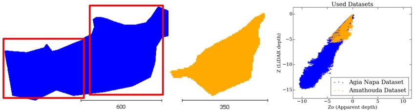
You can also read