Analysis of the Possibility of Using the Plain CFD Model to Simulate Two-Phase Flows in Spatial Systems of Pressure Sewer Networks - MDPI
←
→
Page content transcription
If your browser does not render page correctly, please read the page content below
water
Article
Analysis of the Possibility of Using the Plain CFD
Model to Simulate Two-Phase Flows in Spatial
Systems of Pressure Sewer Networks
Piotr Siwicki 1, * , Marcin Krukowski 1 , Jan Studziński 2 , Bartosz Szelag
                                                                           ˛ 3 and
Rafał Wojciechowski   4

 1   Faculty of Civil and Environmental Engineering, Warsaw University of Life Sciences SGGW,
     PL 00-090 Warsaw, Poland; marcin_krukowski@sggw.edu.pl
 2   Systems Research Institute PAN, PL 00-090 Warsaw, Poland; Jan.Studzinski@ibspan.waw.pl
 3   Faculty of Environmental, Geomatic and Energy Engineering, Kielce University of Technology,
     PL 25-116 Kielce, Poland; bszelag@tu.kielce.pl
 4   EkoWodrol Sp. z o.o., PL 75-209 Koszalin, Poland; rafal.wojciechowski@ekowodrol.eu
 *   Correspondence: piotr_siwicki@sggw.edu.pl; Tel.: +48-22-5935293

 Received: 20 May 2020; Accepted: 19 June 2020; Published: 22 June 2020

 Abstract: The paper analyzes the possibility of using the CFD (Computational Fluid Dynamics)
 method to predict the amount of sewage remaining in siphons after a full air blast of the pressure
 sewer system. For this purpose, the results from measurements carried out on a laboratory installation
 were compared with the results obtained from modelling using a spatial model (3D) and a plain
 model (2D) of the installation. To determine these models, the structure of the VOF (Volume of Fluid)
 model was used in the CFD method. The simulation calculations carried out make it possible to state
 that the use of the plain model with the development of the installation modelled in the plan does
 not result in significant deterioration of the obtained results. The possibility of using 2D models for
 modelling pumped sewer systems allows for a significant shortening of the calculation time, which,
 in practice, results in the possibility of modelling much larger and longer installations than is possible
 with 3D models.

 Keywords: pressure sewer installations; siphons; laboratory tests; CFD modeling; volume of fluid
 (VOF) method

1. Introduction
     In the last few years, there has been a significant development of pressure sewer systems due to the
need to adapt designed installations to the difficult topographic conditions in which they operate, such as:
a small slope of the terrain; striped buildings; rocky ground; and unfavorable ground conditions with high
groundwater levels [1–6]. The main advantage of such installations is the tightness of the pipeline and the
resulting lower odor nuisance of pumped wastewater. Moreover, such sewer systems are characterized
by a simpler construction than gravity systems and are cheaper to implement [7,8].
     However, during the operation of a pressure sewer system, usually the sewage inside the pipeline
is crumpled due to the lack of air access, and dangerous toxic volatile substances are released in
expansion wells [9]. This means that the pressure sewer system eliminates the release of odors along
the length of the pipeline, but leads to a dangerous situation of hydrogen sulfide release at the end
of the pipeline. Hydrogen sulfide in small concentrations causes odor discomfort, while in large
concentrations, it is poisonous and may even threaten the lives of waterworks workers.
     This phenomenon is prevented by shortening the time of sewage retention in the pipeline,
the blowing of compressed air, or the addition of chemical reagents to the sewage. The use of blowing

Water 2020, 12, 1779; doi:10.3390/w12061779                                      www.mdpi.com/journal/water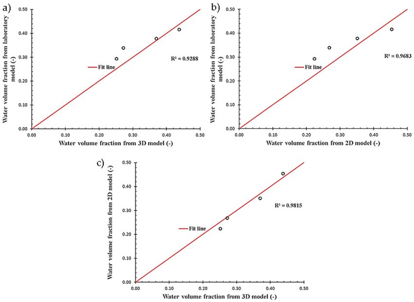
Water 2020, 12, 1779                                                                                2 of 14

is a very common and radical method, because the rotten wastewater deposited in the pressure
pipe is completely removed from it. This method was used as early as 1942 in sewage systems in
California [10].
     The method, however, causes some problems when introducing wastewater into the pipeline
after the blowing, due to the pipeline profile. The pressure pipe is usually not horizontal in length,
but has various, sometimes large slopes and elevations due to the land obstacles that it has to overcome.
This results in a number of points with very different elevation coordinates in its profile, where siphons
and so-called pipe tops are located.
     There is usually some volume of sewage remaining in these siphons, while air accumulates at
the top of the pipeline, forming so-called air bags. Wastewater remains in the siphons, i.e., in local
pipe minima, and air bags in the upper parts of the pipes, i.e., in local pipe maxima, have an adverse
effect on the pressure distribution in the pipeline when the wastewater is once again pumped into
the pipeline, and consequently on the operation of the pumps in the source well and on the flow of
wastewater in the pipe [11].
     Air remaining in the upper parts cause hydraulic hammers in the pipeline and lead to a temporary
two-phase flow and a turbulent flow with respect to wastewater. In order to limit such situations
as much as possible by controlling the pump operation, it is important to correctly recognize the
phenomena of sewage leaching from siphons, and air bags leaching from the tops of the pressure pipe.
For this purpose, accurate models of the sewer pressure pipes and the processes that take place in
them during air blowing and when pumping wastewater after blowing should be developed. This is a
contemporary challenge in sanitary engineering, in which various research facilities are involved by
carrying out appropriate laboratory tests, e.g., in Spain [12].
     The paper deals with the problem by using the CFD (Computational Fluid Dynamics) method to
model the pressure pipeline of aerated wastewater. The model was calibrated on the basis of real data
obtained from measurement experiments carried out on a laboratory installation made especially for
this purpose in the Environmental Engineering Company EkoWodrol in Koszalin (Poland).
     The CFD method is used to create numerical models of the examined environmental processes
and is very accurate, though its applicability is limited in the case of modelling complex processes,
which include two-phase flow phenomena occurring in pressure sewer pipes. The calculation of
spatial models of such processes requires very long calculation times, especially when the model takes
into account the variable hydraulic and geometric conditions of the installation under investigation.
The pipelines of pressure installations have lengths ranging from several hundred meters to several or
even several dozen kilometers, and spatial models of such installations require such long calculation
times that they are unacceptable in practice.
     Therefore, using access to measurements from the laboratory installation, a 3D spatial model was
developed and calibrated for it and then, on the basis of this model, 3D and 2D models were developed
for a section of the installation containing a siphon. This made it possible to thoroughly examine the
process of leaching the liquid from the siphon during blowing of the pipe with compressed air, and thus
examining one of the two key and previously mentioned processes taking place in the pressure sewer.
The 2D model requires much less work and calculation time than the 3D model. With results obtained
for both models, it was possible to assess whether it is possible to replace the spatial model with
a plain model while maintaining satisfactory calculation accuracy and, at the same time, checking
whether the calculation times obtained with the 2D model are acceptable from the point of view of
calculation practice.
     Investigating the processes of flow and aeration of wastewater in pressure pipes by means of
measurement experiments and mathematical modelling is of cognitive value, but most importantly,
it enables the development of algorithms to control these processes in such a way as to eliminate
the phenomenon of wastewater crushing in pipes and the formation of toxic or, at best, bothersome
hydrogen sulfide evaporations.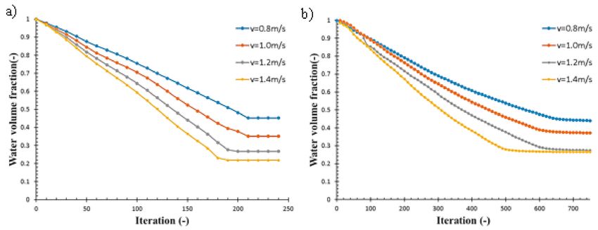
Water 2020, 12, 1779 3 of 14
At the same time, it should be noted that adequate aeration of a pressure sewerage system
leads to an improvement in the quality of wastewater entering the sewage treatment plant, which
has a positive impact on the operation of the plant and on the reduction of pollutant concentrations
in treated wastewater. The effect of cyclic aeration of wastewater in sewage pipes is a reduction
in the amount of excessive sludge generated in the treatment process, a reduction in the degree of
internal sewage recirculation and a reduction in the amount of oxygen supplied to the activated sludge
chambers. Reducing the degree of sewage recirculation and reducing the amount of oxygen pumped
by wastewater blowers into the bioreactor reduces the electricity consumption of energy-intensive
plant facilities. On the other hand, the reduction in the amount of excessive sludge produced by the
plant makes it possible to plan less material-intensive activated sludge chambers of smaller capacity at
the plant design stage.
From the above, it can be seen that the modeling of sewage pressure systems, creating the basis
for the next stage of the development of sewage aeration algorithms, is important both for research as
well as for economic and environmental reasons, which is an argument for the purposefulness and
even the necessity of such research.
2. Materials and Methods
Modelling of the sewage pressure pipeline consisted of three stages. In the first stage of the work,
a 3D spatial model of a 100 m long laboratory installation was made and its hydraulic calibration was
carried out under conditions of liquid flowing in the installation without air. To develop the model of
the installation, the CFD method using the VOF (Volume of Fluid) model was applied [13,14].
In the second stage of research, 3D and 2D models were formulated for a fictitious installation
with a siphon, also 100 m long, into which compressed air was entered to test the process of leaching
the liquid from the siphon. The main aim of this study was to compare the calculation times obtained
for the spatial and plain model.
Finally, in the third stage of the research, a section of the pipe containing a siphon was separated
from the laboratory installation in order to enable the testing of the phenomenon of leaching the liquid
from the siphon at different speeds of the air intake on the basis of this section. For the extracted section
of the installation, with a length of 19.83 m, 2D and 3D models were again determined for different air
velocities and the modelling results obtained with these models were compared for both accuracy and
calculation time.
2.1. Laboratory Installation
The laboratory installation was completed in EkoWodrol’s laboratory in Koszalin as a part of a
research project “Development of an innovative device for flushing and aerating the sewer pressure
pipeline with compressed air limiting the processes of wastewater crushing”, financed by the Polish
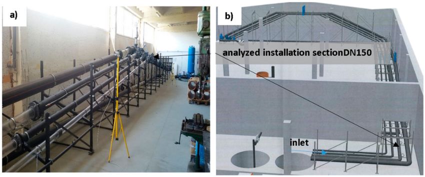
National Research and Development Centre (NCBR) (Figure 1).
Figure 1. View of laboratory installation for testing processes in pressure sewerage pipelines; (a) general
view (left), (b) diagram of the route and profile of the pressure pipeline with indication of the tested
section with a siphon (right).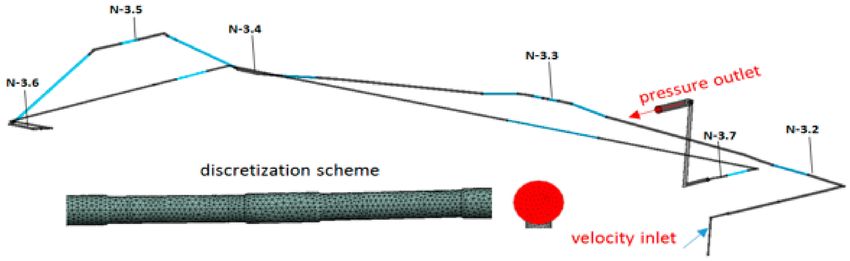
Water 2020, 12, 1779                                                                                           4 of 14

     The model of the whole installation was made for a DN150 diameter and a 100 m long pressure
pipeline. In the case of modelling a section of the installation with a siphon, the pressure pipeline
included in the model has a length of L = 19.83 m and the slope of its ascending segment coming out of
the siphon is 6◦ (Figures 1 and 2).

      Figure 2. Profile of the analyzed installation section with a siphon 19.83 m in length; the liquid flow is
      from left to right.

      The measurement experiments carried out on the laboratory installation were as follows:

•    The first stage of the tests consisted in filling the installation with water and removing air from it
     using vent valves.
•    Then the stage of calibration of the 3D model of the whole installation was followed by adjusting
     the roughness coefficient values of the pipe so that the pressure values calculated by the model
     coincided with the pressure values recorded in the measurement points located on the installation
     (Figure 3).
•    During these tests, water was pumped into the pipeline at a speed of 0.7 m/s.

      Figure 3. Geometry and method of discretization of the 3D model of the entire 100 m long
      laboratory installation.

     Next, after switching off the pump, it was waited until the pressure in the pipeline had stabilized,
and, when this happened, the next stage of testing was started with the introduction of air into the pipe.

•     The air was introduced at point D-1.3 (Figure 2) and its feeding was completed after 30 s from the
      moment when air got through the highest point in the siphon; the volume of water remaining
      in the siphon after such a blow-out was measured by draining water from the trap with a drain
      valve (Figure 2).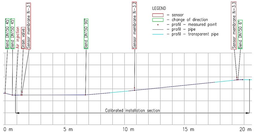
Water 2020, 12, 1779                                                                                        5 of 14

•     The air was introduced into the pipe at four speeds used in the operating practice of water supply
      companies during the blow-out of the pressure systems: v = 0.8; 1.0; 1.2; 1.4 m/s.
•     The aim of this stage was to test the process of leaching liquids from the siphons during the
      blow-out of the pressure pipelines.

      The use of water in research instead of sewage was caused by environmental restrictions.

2.2. Numerical Model
     The CFD method (computational fluid dynamics) and the Fluent program [15] were used to
numerically simulate laboratory installation models. To solve the model equations, the Finite Element
Method has been applied [16,17]. It is an approximate method to solve partial differential equations
describing a control volume of fluid flowing in a modelled pipe. The differential equations in the
CFD method are, in general, a mathematical description of the fundamental laws of mass, momentum
and energy preservation defining the flow of fluids [18]. Regardless of the type of fluid movement
(laminar or turbulent), the following flow continuity equation and momentum equation should always
be solved [19–21]:
     Flow continuity equation:
                                              ∂ρ ∂ui
                                                 +      =0                                        (1)
                                              ∂t    ∂xi
where: t—time [s], u: fluid velocity [m/s], ρ: fluid density [kg/m3 ] and ui is the velocity component in
the xi -direction (i.e., u and v in the horizontal x and the vertical y directions, respectively).
     Momentum Equation (Navier–Stokes) describing the changes in the speed field:

                        ∂ ρui      ∂             ∂       ∂ui    ∂u j     ∂p    ∂τij
                                                      "               !#

                                +      ρui u j =        µ      +        −     +      +F                        (2)
                           ∂t     ∂x j           ∂x j     ∂x j   ∂xi      ∂xi   ∂x j

where p: hydrostatic pressure, µ: dynamic viscosity, τij : strain tensor, ρg: mass forces, F: surface forces.
The components (p, u) in the equation are averaged.
     The strain tensor is defined by the following relationship:

                                                            ∂ui    ∂u j
                                                                        !
                                                                           2
                                   τij =   −ρu0i u0j   = µt      +        − ρδij k                             (3)
                                                            ∂x j   ∂xi     3

where ρu0i u0j : called the Reynolds stresses [4], µt : eddy viscosity and k = (ui uj )/2 is the turbulent kinetic
energy per unit mass. There is also a kinematic turbulent or eddy viscosity denoted by νt = µt /ρ, with
dimensions m2 /s; δij is the Kronecker delta (δij = 1 if i = j and δij = 0 if i , j).
    The averaged Navier–Stokes Equations [22] for the stationary flow of liquid can be written for a
coordinate as follows:
                                                       ∂u j
                                                            =0                                                 (4)
                                                       ∂xi
                           ∂              ∂p     ∂               ∂ui    ∂u j      2 ∂
                                                      "                       !#

                               ρui u j = −     +        (µ + µt )      +         −       (ρk)                  (5)
                          ∂x j             ∂xi   ∂x j             ∂x j   ∂xi       3 ∂xi
where, ui : averaged velocity vectors, µt : turbulent viscosity, k: kinetic turbulent energy, i,j = 1,2,3.
     Equation (5), by taking into account the turbulent viscosity µt , is a description of the transient
flow occurring during the mixing of fluids in a two-phase flow. When dealing with a turbulent flow,
the transport Equation must also be included in its description. In such a case, the k-ε standard
model [15] is most commonly used. The models belonging to the k-ε group are semi-empirical models
described by Equations (6) and (7), where one Equation describes the transport of kinetic turbulent
energy k [23] and the other describes the dissipation of energy ε. These Equations have been derived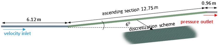
Water 2020, 12, 1779 6 of 14
assuming the isotropy of turbulence, whereby this assumption requires the definition of the following
additional dependencies for wall flows.
The following transport equation was used in our calculations:
∂ ∂ ∂k ∂ui ∂u j ∂ui
" # !
ρku j = µ + µt + µt + − ρε (6)
∂x j xj ∂x j ∂x j ∂xi ∂x j
∂ ∂ ∂k ∂ui ∂u j ∂ui ε ε2
" # !
ρεu j = µ + µt + Cε1 µt + − Cε2 ρ (7)
∂x j xj ∂x j ∂x j ∂xi ∂x j k k
In Equations (6) and (7), the parameters k and ε are linked by the following phenomenological
relationship, based on the observation of real flows:
k3/2
ε= (8)
L
where ε: dissipation of kinetic turbulent energy, L: length scale, which may be expressed by the
hydraulic radius L = 0.07D [15].
Relation (8) results from the Kolmogorov model [24], which assumes that the kinetic energy of
turbulence k is transferred from large scale whirlpools to small scale whirlpools where it is dissipated.
The unknowns in the transport Equation are calculated based on the following relationship
described in [25]:
k2
µt = Cµ ρk1/2 L = Cµ ρ (9)
ε
Universal constant values for incompressible liquids Cµ, Cε1 and Cε2 in Equations (7) and (9)
are determined experimentally. The following values of these coefficients were determined in our
calculations: Cµ = 0.009, Cε1 = 1.44 and Cε2 = 1.92 [15].
2.2.1. Multi-Phase Flows
CFD methods enable the modelling of many types of multiphase flows, in which the following
combinations of flowing fluids can generally be distinguished: gas-liquid, liquid-liquid, gas-solid,
liquid-solid for two-phase flows and gas-liquid-solid for three-phase flows. Two versions of the CFD
method are currently used to numerically solve multiphase flow Equations: The Euler–Lagrange
method and the Euler–Euler method [15,17,26,27].
Our calculations use the Euler–Euler method, which assumes that all the phases considered are
treated as mutually interpenetrating continuums. This method can use different descriptions of created
models: the Volume of Fluid model (VOF), the Mixture model and the Eulerian model. The VOF
model was used in the calculations. This model is one of many commonly used proposals for the
reconstruction of the interfacial surface based on the balancing of a certain additionally accepted
quantities: phase content fraction αq [15]. The αq function is a scalar function assuming values from 0
to 1, depending on the volume amount of a given phase f in the control fluid volume.
The tracking of the interface between the phases is accomplished by the solution of a continuity
Equation [5] for the volume fraction of one (or more) of the phases. For the qth phase (10), this Equation
has the following form:
n
1 ∂ X
αq ρq + ∇· αq ρq uq = S∝q + mpq − mqp (10)
ρq ∂t
p=1
where mqp is the mass transfer from phase q to phase p and mpq is the mass transfer from phase p to
phase q. By default, the source term on the right-hand side of Equation (10), Sαq , is to specify a constant
or user-defined mass source for each phase.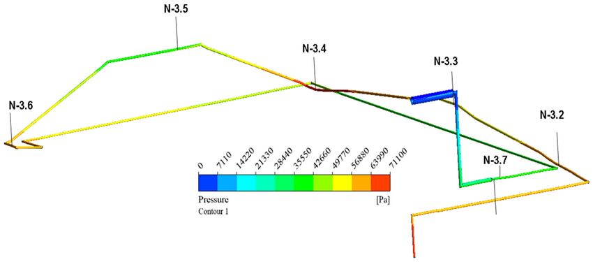
Water 2020, 12, 1779                                                                                  7 of 14

     The volume fraction Equation will not be solved for the primary phase; the primary-phase volume
fraction will be computed based on the following constraint (11):
                                                 n
                                                 X
                                                       αq = 1                                           (11)
                                                 q=1

     Based on the knowledge of the solution of Equation (11), i.e., the distribution of values and gradient
αq in space, the actual surface defined as a functional layer with αq value equal to 12 is reconstructed,
assuming arbitrarily that this value best approximates the position of the interphase boundary.
     From among a number of available algorithms used to reconstruct this surface, an algorithm
based on a linear interpolation of α values, called the geometric reconstruction scheme, was selected
for calculation. In the first stage of calculations, it determines the positions of the layered points on the
edges of finite elements by means of linear interpolation. The second stage of the calculation consists
of determining the surface based on the marching cubes algorithm.
     This algorithm, widely used in the field of three-dimensional space graphics, allows for the quick
and effective determination of the surface, with accuracy limited to the size of a single finite element.
The resulting geometric structure, consisting of triangles, approximates the actual geometry of the
interfacial surface.
     The modelling calculations were carried out under steady state conditions, thus obtaining
approximate solutions. This way the solutions of the above equations were obtained faster than using
transient (transident) modelling. However, the adoption of this modelling approach did not allow for
the use of real time steps in the calculations, forcing only iterative steps to be taken into account, which
meant that it was not possible to trace the changes in the process of the leaching of liquids from the
siphon on the numerical model in real time.

2.2.2. Boundary Condition
     Defining boundary conditions is one of the most important tasks when performing CFD analyses.
The following boundary conditions were used in the models under study:

–     the inlet to the model was defined as a function velocity inlet, in which a constant value of
      velocity (of liquid or gas in case of blowing) was given, without giving the velocity profile in the
      cross-section of the modelled pipeline; the volume fraction for the primary phase q (air) was equal
      to 0 for water or 1 for air; the turbulence parameters length scale and hydraulic diameter were
      adopted as the specification of transported turbulence quantities;
–     on the wall of the pipeline, adopting the standard wall roughness models [15], the concept of the
      boundary layer was used, assuming the change of velocity profile in turbulent flow near the wall,
–     the values of viscosity and density of liquids were assumed for liquids (water), and for gas (air);
–     the model outlet was defined as a pressure outlet function; the turbulence parameters length scale
      and hydraulic diameter were adopted as the specification of transported turbulence quantities.

2.3. Spatial Model (3D) of the Installation
     On the basis of the technical documentation of the 100 m long laboratory installation, its spatial 3D
model was developed (Figure 3). For this model, a spatial calculation grid was defined, consisting of
1,888,302 knots and 1,521,879 elements. An average grid quality index of 0.83 was obtained, while the
maximum value of this indicator is 1. To carry out calculations with such a large number of elements,
16 processors with a 2.4 GHz clock frequency were used.
     The boundary condition at the point of pumping water into the installation (inlet) was defined in
the model as a velocity-inlet function of the FLUENT program, and, at this point, the value of water
flow velocity was defined. The boundary condition at the point of water outflow from the installation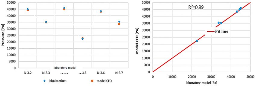
Water 2020, 12, 1779                                                                                 8 of 14

(outlet) was defined in the model as a pressure-outlet, meaning free flow. Using the function wall,
the pipe walls were defined.
     During the calibration of the model of the sewer pipeline, a value of the coefficient of pipeline
roughness equal to 0.0001 m was determined. The calculated pressure values were recorded at the same
points of the model where the pressure sensors on the laboratory installation are located (Figure 3).

2.4. Spatial Siphon Model (3D)
     On the basis of the profile of the entire laboratory installation (Figure 2), a 19.83 m long section of
the installation containing a siphon has been extracted, and a 3D spatial model has been developed for
this pipeline fragment.
     The modelled section of the installation has a diameter of DN150, with the slope of the ascending
pipe being 6◦ (Figure 4). For the model being created, a spatial calculation grid has been defined,
consisting of 2,327,135 knots and 1,583,009 elements. An average grid quality index of 0.96 was obtained.

      Figure 4. Geometry and method of discretization of the 3D model of the 19.83 m long installation
      section containing the siphon.

     The boundary conditions in the model were defined by assuming the function velocity inlet,
where the air was introduced with different velocity values assumed, while the model outlet was
defined as the function pressure outlet. For pipeline walls the function wall was assumed. The value
of roughness coefficient determined for the pipe is equal to k = 0.0001 m.

2.5. Plain Siphon Model (2D)
     By creating a 2D model for the pipeline with a siphon, the relevant spatial fragment of the
installation is presented on the plane while respecting the length of individual pipeline sections
(Figure 5). On the basis of the flat profile of the pipeline obtained in this way, a two-dimensional model
was developed, whose calculation grid consists of 27,236 knots and 25,587 elements. An average grid
quality index of 0.98 was obtained.

      Figure 5. Geometry and method of discretization of the 2D model of the 19.83 m long installation
      section containing the siphon.

     Similar to the 3D model, the length of the modelled pipeline is 19.83 m, the pipe has a diameter of
DN150, the slope of the ascending section is 60 and the pipeline roughness coefficient is k = 0.0001 m.
The functions velocity inlet, pressure outlet and wall are assumed for the inlet, outlet and wall of the
modelled pipeline respectively.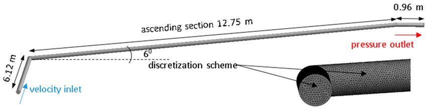
Water 2020, 12, 1779                                                                                      9 of 14

3. Results
     In the first phase of research, a 3D model of the laboratory installation was developed and
calibrated on the basis of pressure measurements from six measurement points installed on the
installation (Figure 3). The results from the model simulation (Figure 6) were compared with the
measurement results leading to their convergence by choosing the value of the roughness coefficient of
the pressure pipe. Pressure values from sensors N-3.2, N-3.3, N-3.4, N-3.5, N-3.6 and N-3.7, located
virtually in the model and physically on the pipeline, were analyzed. For comparison of the calculated
and measured pressures, the average values determined over a water flow duration of 103 s were
taken into account. The average water flow value determined from the flow meter installed in the
source well of the installation, equal to 18.52 m3 /h, was also considered in the calibration calculations.

      Figure 6. Pressure distribution obtained during calibration of the CFD model of the entire 100 m long
      laboratory installation.

      During the calibration of the model, a high correlation between the results of the calculation and
the measurements was obtained, assessed on the basis of the correlation coefficient. For the calibrated
model, a value of this coefficient equal to R2 = 0.99 was obtained (Figure 7). Only for the sensor N-3.7,
placed close to the outlet of the installation, was greatest difference in pressure values measured and
calculated at the level of 2% obtained, which results from the unsteady flow conditions at this point of
the pipeline. This is evidenced by the oscillations in the readings of the momentary flow values from
the flow meter installed at the outlet of the installation.

      Figure 7. Comparison of pressure values obtained from the CFD model with the results obtained from
      the measurements.

     The time of a single simulation of the 3D model for the 100 m long installation during the model
calibration was 48 h. A PC with 16 processors and with a 2.4 GHz clock frequency was used to carry
out the calculations and water was pumped into the pipeline at a velocity of 0.7 m/s.
     In the next phase of research, 3D and 2D models were used to carry out simulations for a fictitious
100 m long pipe with a siphon, including wastewater aeration, i.e., a two-phase flow in the pressure
Water 2020, 12, 1779 10 of 14
pipe was already modeled. In this study, the process of leaching the liquid from the siphon of the
pipeline during its blowing with compressed air, pumped into the pipe at a velocity of 0.8 m/s was
analyzed. Modelling calculations were carried out until the moment when the injected air reached the
outlet of the pipeline. The purpose of these calculations was to check what impact the replacement
of a complex 3D model with a simpler 2D model has on reducing the calculation time. It turned out
that this impact is very high because the simulation of two-phase flow for the tested pipeline using
the 3D model required a calculation time of 168 h, while for the 2D model this time was 24 h, which
was seven times shorter. It can be noted that the time of two-phase flow modeling has significantly
increased compared to single-phase flow modeling: a single simulation of a 3D model for a 100 m
long laboratory installation for single-phase flow was 48 h, while for a 100 m long pipeline, but for
two-phase flow, it was as much as 168 h.
In the last phase of research, using 3D and 2D models, simulation calculations were performed for a
selected section of a 19.83 m long laboratory installation, analyzing, as before, the process of leaching the
liquid from the siphon of the pipeline during its blowing with compressed air. This time, a two-phase flow
in the pipe was once again modeled. The aim of this phase of research was twofold. On the one hand,
it aimed to determine the influence that the process of leaching the liquid from the installation siphon has
on the velocity of air entering the pipeline, with the second equally important aim of the research being
the assessment of the impact of replacing the 3D model with a 2D model on the accuracy of calculations.
Measurement experiments carried out on the laboratory installation and calculation experiments carried
out with the use of the models consisted in pressing air into the pipeline at different velocities of 0.8, 1.0,
1.2 and 1.4 m/s and analyzing the amount of water remaining in the siphon. The process of leaching water
from the siphon was carried out on the installation and simulated with the use of models until the entered
air reached the outlet section of the tested pipe. At this stage, the simulation was completed and the
amount of water remaining was estimated. This means that, as before, the experiment was stopped after
the air passed through the analyzed syphon section.
To determine the amount of water remaining in the siphon in the case of the laboratory installation
and the 3D model, a dimensionless factor was defined, expressing the ratio of the volume of the pipe
occupied by the water to the geometric volume of the analyzed section of the installation.
In the case of the 2D model, a coefficient has been defined expressing the ratio of the field occupied
by water to the field of the analyzed section of the installation.
The results of the measurement experiments and calculations performed have been presented in
Table 1.
Table 1. Values of the residual water volume in the siphon obtained from the measurements and
modelling calculations.
Velocity (m/s) Amount of Water Remaining (l) Water Volume Fraction (-)
Laboratory test
0.80 145.60 0.42
1.00 132.30 0.38
1.20 118.65 0.34
1.40 102.55 0.29
CFD model 3D
0.80 153.30 0.44
1.00 129.50 0.37
1.20 95.20 0.27
1.40 88.20 0.25
CFD model 2D
0.80 - 0.45
1.00 - 0.35
1.20 - 0.27
1.40 - 0.22Water 2020, 12, 1779 11 of 14
Calculations carried out with the help of 3D and 2D numerical models allowed to observe the
variability of the water volume in the siphon during the pumping of air into the pipe (Figure 8).
The results of the calculations show that the process of leaching the liquid from the siphon of the
pressure pipe simulated by means of both models is very similar, which means that the application of
2D modelling generally gives a similar calculation accuracy to that of 3D modelling, at least for the
tested two-phase flow in the pressure pipeline.
Figure 8. Variability of water volume remaining in the installation during the air blow-out obtained
from calculations carried out using: (a) 2D model, (b) 3D model.
The comparison of the calculation results obtained for both models with the measurements is
shown in Figure 9. Both the CFD 3D spatial model and the 2D plain model overstate the amount
of water remaining in the installation at the assumed maximum blowing speed of 1.4 m/s. For the
remaining blowing speeds, the determined volume of water remaining in the siphon is slightly lower
than in reality. Despite some discrepancies between the measurement results and the results obtained
from the numerical models of the installation, high values of correlation coefficients were obtained for
all analyzed cases.
Figure 9. Comparison of modelling results with measurement results: (a) 3D model vs. measurements,
(b) 2D model vs. measurements, (c) 3D model vs. 2D model.Water 2020, 12, 1779 12 of 14
The correlation between the measurements from the installation and the results of the 3D model
was R2 = 0.9288, with that for the 2D model at R2 = 0.9683; the highest correlation coefficient was
obtained between the results of the calculations of both models, equal to R2 = 0.9815.
On the basis of the calculations carried out, it can be concluded that, in the analyzed flow
and blowing conditions, the modelling of sewage pressure pipes with the CFD method is justified.
The obtained results of calculations concerning the leaching of sewage from the installation siphons
during blowing with compressed air are very similar to the results obtained from measurements on
real installations.
Moreover, it is justified and advisable to use 2D plain models in such cases, seeing as how the
results obtained with their use only slightly deviate from the results obtained with 3D spatial models.
At the same time, a very important argument in favor of using 2D modeling to simulate two-phase
flows in pressure pipelines is the significant reduction in calculation time compared to 3D modelling.
When modelling an isolated 19.83 m long section of the installation with an air velocity of 0.8 m/s,
calculation times of 1 h for the 2D model and 7 h for the 3D model were obtained. A calculation time
of 1 h is acceptable in calculation practice. At the same time, the obtained results indicate that it is
advisable and justified, for the sake of time saving, not only to use 2D for the simulation of two-phase
flows in pressure pipes, but also to model selected characteristic flow processes for only selected parts
of the pipelines as opposed to the entire sewage system.
4. Discussion
In order to improve the quality of wastewater in pressure sewer networks, it is common practice
to use compressed air blowing to break the biological film from the pipeline walls and to aerate the
wastewater. In the case of full blowing, sewage stoppers are formed at the points of change of the
network route (siphons), from which the sewage is not completely leached. The amount of sewage
remaining in the installation generates additional pressure in the pipeline and its amount affects pump
operation parameters when the sewage is once again pumped into the installation.
High convergence of the results of measurements conducted on the laboratory installation
(physical model) with the results obtained by means of the numerical models indicate the usefulness
of the CFD method in determining the amount of sewage remaining in siphons after a full blow of the
installation. The use of the VOF model for 3D and plain 2D spatial modelling gives results similar to
those obtained from the laboratory installation.
The use of a flat model (2D) with the installation development in the plan does not significantly
affect the results obtained from the spatial model (3D). At the same time, the possibility of using a
2D model for modelling pressure sewage systems allows for the significant reduction of calculation
time and, as a result, enables the modelling of much larger and longer sections of installations than is
practically possible with a 3D model.
At the same time, it is important to stress the importance and advisability of conducting research
related to modelling the flow and aeration of wastewater in pressure pipelines. Such research is
not only scientific in nature, but also very practical, as it enables the development of algorithms for
controlling the aeration of the pressure canalization in such a way as to eliminate the crushing of
sewage and the formation of bad odors that are potentially harmful to health. At the same time,
appropriate aeration of wastewater in pressure pipes has a positive impact on the operation of
wastewater treatment plants, minimizing their electricity consumption and having a positive impact
on the quality of treatment by supporting the process of reducing pollution in wastewater, which has
important ecological significance.Water 2020, 12, 1779 13 of 14
Author Contributions: Conceptualization, P.S., methodology, P.S., M.K., J.S., B.S.; formal analysis, P.S., M.K., J.S.,
B.S.; writing—original draft preparation P.S., M.K., J.S., B.S.; writing—review and editing, P.S., M.K., J.S., B.S. and
R.W.; visualization, P.S., M.K., J.S., B.S. and R.W.; supervision, P.S., M.K., J.S., B.S. and R.W.; All authors have read
and agreed to the published version of the manuscript.
Funding: Measurement data, on the basis of which modelling calculations were made, were obtained during
experiments carried out at EkoWodrol in Koszalin/Poland under the research project No. 01/11/2016/NCBR
entitled: “Development of an innovative device for flushing and aeration of wastewater pressure pipeline with
compressed air, limiting the processes of wastewater crushing”, co-financed by the Polish National Centre for
Research and Development.
Conflicts of Interest: The authors declare no conflict of interest.
References
1. Kasprzyk, M. Analiza Systemu Kanalizacji Podciśnieniowej (Analysis of Underpressure Sewer Systems);
Gdansk University of Technology: Gdansk, Poland, 2017; Available online: https://www.researchgate.net/
publication/324221767_Analiza_systemu_kanalizacji_podcisnieniowej (accessed on 9 May 2020).
2. The Sewer Battle: Gravity, vs. Pressurized. Available online: https://www.mswmag.com/online_exclusives/
2014/08/the_sewer_battle_gravity_vs._pressurized (accessed on 10 May 2020).
3. Kalenik, M. Niekonwencjonalne Systemy Kanalizacji (Unconventional Sewerage Systems); Wydawnictwo SGGW:
Warsaw, Poland, 2011.
4. Kotowski, A. Podstawy Bezpiecznego Wymiarowania Odwodnień Terenów. Sieci Kanalizacyjne (The Basis for Safe
Dimensioning of Land Drainage. Wastewater Networks); Wydawnictwo Seidel-Przywecki Sp. z.o.o.: Warsaw,
Poland, 2015.
5. Łomotowski, J. System kanalizacji ciśnieniowej (Pressure sewer system). Wodociagi ˛ I Kanaliz. 2006, 5, 27.
6. McAllister, E.W. Pipeline Rules of Thumb Handbook: A Manual of Quick, Accurate Solutions to Everyday Pipeline
Engineering Problems; Gulf Professional Publishing: Waltham, MA, USA, 2015.
7. Huskie, S. Overview of Low Pressure and Small Diameter Gravity Sewers; United States Environmental Protection
Agency: Stony Point, NY, USA, 2000.
8. Thrasher, D. Design and Use of Pressure Sewer System; Lewis Publishers, Inc.: Chelsea, MI, USA, 1988.
9. Stachowiak, M.; Troszczyńska, M.; Dymaczewski, Z. Przeciwdziałanie Uciażliwości
˛ Odorowej w Systemach
Kanalizacji Grawitacyjno-Tłocznej (Preventing Odour Problems in Gravity and Pressure Sewer Systems);
Technologia Wody nr 56 (6); Wydawnictwo Seidel-Przywecki Sp. z.o.o.: Warsaw, Poland, 2017.
10. Hvitved-Jacobsen, T.; Vollertsen, J.; Nielsen, A.H. Sewer Processes: Microbial and Chemical Process Engineering
of Sewer Networks; CRC Press: Boca Raton, FL, USA, 2013.
11. Tukker, M.; Kooij, K.; Pothof, I. Hydraulic Design and Management of Wastewater Transport Systems;
IWA Publishing: London, UK, 2016.
12. Garcia, J.T.; Vigueras-Rodrigez, A.; Castillo, L.G.; Carrillo, J.M. Evaluation of Sulfide control by Air-Injection
in sewer force mains: Field and laboratory study. Sustainability 2017, 9, 402. [CrossRef]
13. Guerrero, E.; Muñoz, F.; Ratkovich, N. Comparison between eulerian and vof models for two-phase flow
assessment in vertical pipes. CT F Cienc. Tecnol. Futuro 2017, 1, 73–84. [CrossRef]
14. Zhao, Z.H.; Fernando, H.J.S. Numerical modeling of a sagging pipeline using an Eulerian two-phase model.
J. Turbul. 2008, 9, 1–20. [CrossRef]
15. ANSYS Fluent User’s Guide; ANSYS Inc.: Canonsburg, PA, USA, 2019; Available online:
https://ansyshelp.ansys.com/?ReturnUrl=%2FViews%2FSecured%2Fcorp%2Fv201%2Fen%2Fflu_th%
2Fflu_th.html%3Fq%3Dansys%20fluent%20theory%20guide (accessed on 10 May 2020).
16. Girault, V.; Raviart, P.A. Finite element approximation of the Navier-Stokes equations. In Tom 749 z Lecture
Notes in Mathematics; Springer: Berlin/Heidelberg, Germany, 2006.
17. Prince, J.F. Lagrangian and Eulerian Representations of Fluid Flow; Clark Laboratory Woods Hole Oceanographic
Institution: Woods Hole, MA, USA, 2006.
18. Dziubiński, M.; Prywer, J. Mechanika Płynów Dwufazowych (Mechanics of Two-Phase Fluids); Wydawnictwo Naukowe
PWN: Warsaw, Poland, 2017.
19. Ferrari, A.; Jimenez-Martinez, J.; Borgne, T.L.; Méheust, Y.; Lunati, I. Challenges in modeling unstable
two-phase flow experiments in porous micromodels. Water Resour. Res. 2015, 51, 1381–1400. [CrossRef]Water 2020, 12, 1779 14 of 14
20. Johnson, R.W. Handbook of Fluid Dynamics, 2nd ed.; CRC Press: Boca Raton, FL, USA; Taylor & Francis Group:
Oxfordshire, UK, 2016.
21. Versteeg, H.K.; Malalasekera, W. An Introduction to Computational Fluid Dynamics, 2nd ed.; Pearson Education:
London, UK, 2007.
22. Ferziger, J.H.; Peric, M. Computational Methods for Fluid Dynamics; Springer: Berlin/Heidelberg, Germany, 1999.
23. Taylor, G.I. Statistical Theory of Turbulence. II. Proc. R. Soc. Lond. Ser. A 1938, 164. [CrossRef]
24. Kolmogorov, A.N. Dissipation of Energy in Locally Isotropic Turbulence. First Published in Russian in Dokl.
Akad. Nauk SSSR 32(1), 1941; English Translation in Proc. R. Soc. Lond. A, 434(1890). 1991, pp. 15–17.
Available online: hhttp://www.phys.ens.fr/IMG/pdf/kolmogorov41c.pdf (accessed on 10 May 2020).
25. Ratkovich, N.; Majumder, S.K.; Bentzen, T.R. Empirical correlations and CFD siulations of vertical twophase
gas-liquid (Newtonian and non-Newtonian) slug flow compared against experimental data of void fraction.
Chem. Eng. Res. Des. 2013, 91, 988–998. [CrossRef]
26. Kazimierski, Z. Podstawy Mechaniki Płynów i Metod Komputerowej Symulacji Przepływów (Fundamentals of Fluid
Mechanics and Computer Flow Simulation Methods); Politechnika Łódzka: Łódz, Poland, 2004.
27. Kleinstreuer, C. Modern Fluid Dynamics, 2nd ed.; CRC Press: Boca Raton, FL, USA, 2018.
© 2020 by the authors. Licensee MDPI, Basel, Switzerland. This article is an open access
article distributed under the terms and conditions of the Creative Commons Attribution
(CC BY) license (http://creativecommons.org/licenses/by/4.0/).You can also read