REPRESENTATION LEARNING OF MUSIC USING ARTIST LABELS
←
→
Page content transcription
If your browser does not render page correctly, please read the page content below
REPRESENTATION LEARNING OF MUSIC USING ARTIST LABELS

                                                      Jiyoung Park1∗ Jongpil Lee2∗ Jangyeon Park1 Jung-Woo Ha1 Juhan Nam2
                                                                                   1
                                                                                     NAVER Corp.
                                                                    2
                                                                      Graduate School of Culture Technology, KAIST
                                                {j.y.park, jangyeon.park, jungwoo.ha}@navercorp.com, {richter, juhannam}@kaist.ac.kr

                                                                    ABSTRACT                                       unsupervised learning algorithms such as sparse coding
                                                                                                                   [12, 24, 29, 31], K-means [8, 24, 30] and restricted Boltz-
                                            In music domain, feature learning has been conducted                   mann machine [24, 26]. Most of them focused on learn-
                                         mainly in two ways: unsupervised learning based on sparse                 ing a meaningful dictionary on spectrogram by exploiting
                                         representations or supervised learning by semantic labels                 sparsity. While these unsupervised learning approaches are
                                         such as music genre. However, finding discriminative fea-                 promising in that it can exploit abundant unlabeled audio
                                         tures in an unsupervised way is challenging and supervised                data, most of them are limited to single or dual layers,
arXiv:1710.06648v2 [cs.SD] 19 Jun 2018

                                         feature learning using semantic labels may involve noisy                  which are not sufficient to represent complicated feature
                                         or expensive annotation. In this paper, we present a super-               hierarchy in music.
                                         vised feature learning approach using artist labels anno-                     On the other hand, supervised feature learning has been
                                         tated in every single track as objective meta data. We pro-               progressively more explored. An early approach was map-
                                         pose two deep convolutional neural networks (DCNN) to                     ping a single frame of spectrogram to genre or mood labels
                                         learn the deep artist features. One is a plain DCNN trained               via pre-trained deep neural networks and using the hidden-
                                         with the whole artist labels simultaneously, and the other is             unit activations as audio features [11, 27]. More recently,
                                         a Siamese DCNN trained with a subset of the artist labels                 this approach was handled in the context of transfer learn-
                                         based on the artist identity. We apply the trained models to              ing using deep convolutional neural networks (DCNN)
                                         music classification and retrieval tasks in transfer learning             [6, 20]. Leveraging large-scaled datasets and recent ad-
                                         settings. The results show that our approach is compara-                  vances in deep learning, they showed that the hierarchi-
                                         ble to previous state-of-the-art methods, indicating that the             cally learned features can be effective for diverse music
                                         proposed approach captures general music audio features                   classification tasks. However, the semantic labels that they
                                         as much as the models learned with semantic labels. Also,                 use such as genre, mood or other timbre descriptions tend
                                         we discuss the advantages and disadvantages of the two                    to be noisy as they are sometimes ambiguous to annotate
                                         models.                                                                   or tagged from the crowd. Also, high-quality annotation
                                                                                                                   by music experts is known to be highly time-consuming
                                                              1. INTRODUCTION
                                                                                                                   and expensive.
                                         Representation learning or feature learning has been ac-                      Meanwhile, artist labels are the meta data annotated to
                                         tively explored in recent years as an alternative to feature              songs naturally from the album release. They are objective
                                         engineering [1]. The data-driven approach, particularly us-               information with no disagreement. Furthermore, consid-
                                         ing deep neural networks, has been applied to the area of                 ering every artist has his/her own style of music, artist la-
                                         music information retrieval (MIR) as well [14]. In this pa-               bels may be regarded as terms that describe diverse styles
                                         per, we propose a novel audio feature learning method us-                 of music. Thus, if we have a model that can discriminate
                                         ing deep convolutional neural networks and artist labels.                 different artists from music, the model can be assumed to
                                             Early feature learning approaches are mainly based on                 explain various characteristics of the music.
                                         unsupervised learning algorithms. Lee et al. used convolu-                    In this paper, we verify the hypothesis using two DCNN
                                         tional deep belief network to learn structured acoustic pat-              models that are trained to identify the artist from an audio
                                         terns from spectrogram [19]. They showed that the learned                 track. One is the basic DCNN model where the softmax
                                         features achieve higher performance than Mel-Frequency                    output units corresponds to each of artist. The other is the
                                         Cepstral Coefficients (MFCC) in genre and artist clas-                    Siamese DCNN trained with a subset of the artist labels to
                                         sification. Since then, researchers have applied various                  mitigate the excessive size of the output layer in the plain
                                             * Equally contributing authors.                                       DCNN when a large-scale dataset is used. After training
                                                                                                                   the two models, we regard them as a feature extractor and
                                                                                                                   apply artist features to three different genre datasets in two
                                                       c Jiyoung Park, Jongpil Lee, Jangyeon Park, Jung-Woo        experiment settings. First, we directly find similar songs
                                         Ha, Juhan Nam. Licensed under a Creative Commons Attribution 4.0
                                         International License (CC BY 4.0). Attribution: Jiyoung Park, Jongpil
                                                                                                                   using the artist features and K-nearest neighbors. Second,
                                         Lee, Jangyeon Park, Jung-Woo Ha, Juhan Nam. “Representation Learn-        we conduct transfer learning to further adapter the features
                                         ing of Music Using Artist Labels”, 19th International Society for Music   to each of the datasets. The results show that proposed ap-
                                         Information Retrieval Conference, Paris, France, 2018.                    proach captures useful features for unseen audio datasets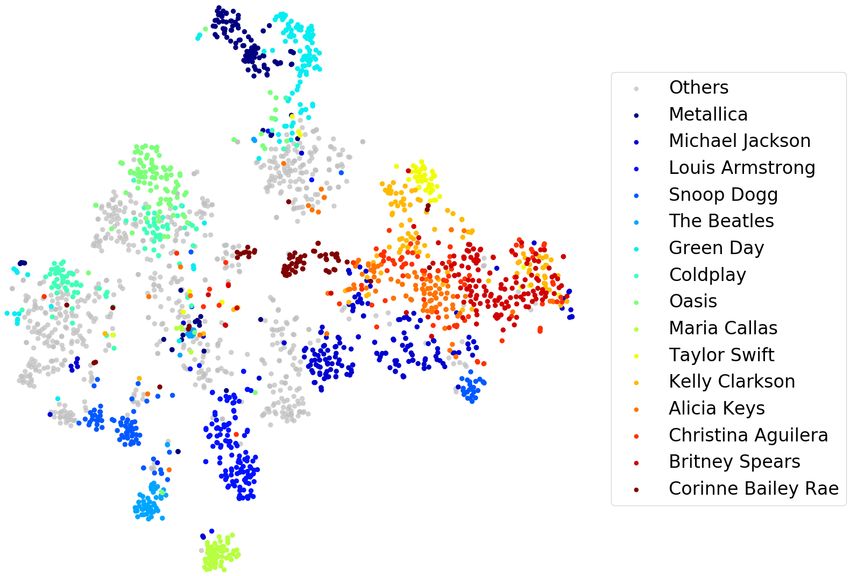
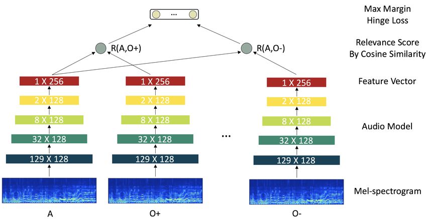
(a) The Basic Model                                       (b) The Siamese Model

                               Figure 1. The proposed architectures for the model using artist labels.

and the propose models are comparable to those trained               dataset has 10,000 artists and the last hidden layer size is
with semantic labels in performance. In addition, we dis-            100, the number of parameters to learn in the last weight
cuss the advantages and disadvantages of the two proposed            matrix will reach 1M. Second, whenever new artists are
DCNN models.                                                         added to the dataset, the model must be trained again en-
                                                                     tirely. We solve the limitations using the Siamese DCNN
                2. LEARNING MODELS                                   model.
Figure 1 shows the two proposed DCNN models to learn                     A Siamese neural network consists of twin networks
audio features using artist labels. The basic model is               that share weights and configuration. It then provides
trained as a standard classification problem. The Siamese            unique inputs to the network and optimizes similarity
model is trained using pair-wise similarity between an an-           scores [3, 18, 22]. This architecture can be extended to use
chor artist and other artists. In this section, we describe          both positive and negative examples at one optimization
them in detail.                                                      step. It is set up to take three examples: anchor item (query
                                                                     song), positive item (relevant song to the query) and nega-
2.1 Basic Model                                                      tive item (different song to the query). This model is often
                                                                     called triplet networks and has been successfully applied to
This is a widely used 1D-CNN model for music classifica-
                                                                     music metric learning when the relative similarity scores of
tion [5, 9, 20, 25]. The model uses mel-spectrogram with
                                                                     song triplets are available [21]. This model can be further
128 bins in the input layer. We configured the DCNN such
                                                                     extended to use several negative samples instead of just one
that one-dimensional convolution layers slide over only a
                                                                     negative in the triplet network. This technique is called
single temporal dimension. The model is composed of 5
                                                                     negative sampling and has been popularly used in word
convolution and max pooling layers as illustrated in Fig-
                                                                     embedding [23] and latent semantic model [13]. By using
ure 1(a). Batch normalization [15] and rectified linear unit
                                                                     this technique, they could effectively approximate the full
(ReLU) activation layer are used after every convolution
                                                                     softmax function when the output class is extremely large
layer. Finally, we used categorical cross entropy loss in the
                                                                     (i.e. 10,000 classes).
prediction layer.
                                                                         We approximate the full softmax output in the basic
    We train the model to classify artists instead of semantic
                                                                     model with the Siamese neural networks using negative
labels used in many music classification tasks. For exam-
                                                                     sampling technique. Regarding the artist labels, we set up
ple, if the number of artists used is 1,000, this becomes
                                                                     the negative sampling by treating identical artist’s song to
a classification problem that identifies one of the 1,000
                                                                     the anchor song as positive sample and other artists’ songs
artists. After training, the extracted 256-dimensional fea-
                                                                     as negative samples. This method is illustrated in Figure
ture vector in the last hidden layer is used as the final audio
                                                                     1(b). Following [13], the relevance score between the an-
feature learned using artist labels. Since this is the repre-
                                                                     chor song feature and other song feature is measured as:
sentation from which the identity is predicted by the lin-
                                                                                                                T
ear softmax classifier, we can regard it as the highest-level                                                  yA yO
                                                                                R(A, O) = cos(yA , yO ) =                     (1)
artist feature.                                                                                              |yA ||yO |
                                                                     where yA and yO are the feature vectors of the anchor song
2.2 Siamese Model
                                                                     and other song, respectively.
While the basic model is simple to train, it has two main               Meanwhile, the choice of loss function is important in
limitations. One is that the output layer can be excessively         this setting. We tested two loss functions. One is the soft-
large if the dataset has numerous artists. For example, if a         max function with categorical cross-entropy loss to max-
imize the positive relationships. The other is the max-           We also should note that the testing set is actually not used
margin hinge loss to set only margins between positive and        in the whole experiments in this paper because we used the
negative examples [10]. In our preliminary experiments,           source dataset only for training the models to use them as
the Siamese model with negative sampling was success-             feature extractors. The reason we filtered and split the data
fully trained only with the max-margin loss function be-          in this way is for future work 2 .
tween the two objectives, which is defined as follows:
                                                                  3.1.2 Tag-label Model
                                                                  We used 5,000 artists set as a baseline experiment setting.
                    X
 loss(A, O) =            max[0, ∆ − R(A, O+ ) + R(A, O− )]
                    O−
                                                                  This contains total 90,000 songs in the training and valida-
                                                         (2)      tion set with a split of 75,000 and 15,000. We thus con-
where ∆ is the margin, O+ and O− denotes positive ex-             structed the same size set for tagging dataset to compare
ample and negative examples, respectively. We also grid-          the artist-label models and the tag-label model. The tags
searched the number of negative samples and the margin,           and songs are first filtered in the same way as the previous
and finally set the number of negative samples to 4 and           works [4, 20]. Among the list with the filtered top 50 used
the margin value ∆ to 0.4. The shared audio model used in         tags, we randomly selected 90,000 songs and split them
this approach is exactly the same configuration as the basic      into the same size as the 5,000 artist set.
model.
                                                                  3.2 Target Tasks
2.3 Compared Model
                                                                  We used 3 different datasets for genre classification.
In order to verify the usefulness of the artist labels and the
presented models, we constructed another model that has                • GTZAN (fault-filtered version) [17, 28]: 930 songs,
the same architecture as the basic model but using semantic              10 genres. We used a “fault-filtered” version of
tags. In this model, the output layer size corresponds to                GTZAN [17] where the dataset was divided to pre-
the number of the tag labels. Hereafter, we categorize all               vent artist repetition in training/validation/test sets.
of them into artist-label model and tag-label model, and
compare the performance.                                               • FMA small [7]: 8,000 songs, 8 balanced genres.

                                                                       • NAVER Music 3 dataset with only Korean artists:
                       3. EXPERIMENTS
                                                                         8,000 songs, 8 balanced genres. We filtered songs
In this section, we describe source datasets to train the two            with only have one genre to clarify the genre char-
artist-label models and one tag-label model. We also in-                 acteristic.
troduce target datasets for evaluating the three models. Fi-
nally, the training details are explained.                        3.3 Training Details

3.1 Source Tasks                                                  For the preprocessing, we computed the spectrogram using
                                                                  1024 samples for FFT with a Hanning window, 512 sam-
All models are trained with the Million Song Dataset              ples for hop size and 22050 Hz as sampling rate. We then
(MSD) [2] along with 30-second 7digital 1 preview clips.          converted it to mel-spectrogram with 128 bins along with
Artist labels are naturally annotated onto every song, thus       a log magnitude compression.
we simply used them. For the tag label, we used the                   We chose 3 seconds as a context window of the DCNN
Last.fm dataset augmented on MSD. This dataset contains           input after a set of experiments to find an optimal length
tag annotation that matches the ID of the MSD.                    that works well in music classification task. Out of the 30-
                                                                  second long audio, we randomly extracted the context size
3.1.1 Artist-label Model
                                                                  audio and put them into the networks as a single exam-
The number of songs that belongs to each artist may be ex-        ple. The input normalization was performed by dividing
tremely skewed and this can make fair comparison among            standard deviation after subtracting mean value across the
the three models difficult. Thus, we selected 20 songs for        training data.
each artist evenly and filtered out the artists who have less         We optimized the loss using stochastic gradient descent
than this. Also, we configured several sets of the artist lists   with 0.9 Nesterov momentum with 1e−6 learning rate de-
to see the effect of the number of artists on the model per-      cay. Dropout 0.5 is applied to the output of the last ac-
formances (500, 1,000, 2,000, 5,000 and 10,000 artists).          tivation layer for all the models. We reduce the learning
We then divided them into 15, 3 and 2 songs for training,         rate when a valid loss has stopped decreasing with the ini-
validation and testing, respectively for the sets contain less    tial learning rate 0.015 for the basic models (both artist-
than 10,000 artists. For the 10,000 artist sets, we parti-        label and tag-label) and 0.1 for the Siamese model. Zero-
tioned them in 17, 1 and 2 songs because once the artists         padding is applied to each convolution layer to maintain its
reach 10,000, the validation set already become 10,000            size.
songs even when we only use 1 song from each artist which            2 All the data splits of the source tasks are available at the link for re-
is already sufficient for validating the model performance.       producible research https://github.com/jiyoungpark527/
                                                                  msd-artist-split.
  1   https://www.7digital.com/                                      3 http://music.naver.com
Our system was implemented in Python 2.7, Keras 2.1.1                              Artist-label     Artist-label   Tag-label
                                                                        MAP
and Tensorflow-gpu 1.4.0 for the back-end of Keras. We                                Basic Model    Siamese Model     Model
used NVIDIA Tesla M40 GPU machines for training our                   GTZAN
                                                                                         0.4968         0.5510         0.5508
models. Code and models are available at the link for re-          (fault-filtered)
                                                                     FMA small           0.2441         0.3203         0.3019
producible research 4 .                                           NAVER Korean           0.3152         0.3577         0.3576

              4. FEATURE EVALUATION                              Table 1. MAP results on feature similarity-based retrieval.
We apply the learned audio features to genre classifica-
                                                                                      Artist-label     Artist-label    Tag-label
tion as a target task in two different approaches: feature            KNN
                                                                                      Basic Model    Siamese Model      Model
similarity-based retrieval and transfer learning. In this sec-
tion, we describe feature extraction and feature evaluation          GTZAN
                                                                                        0.6655           0.6966         0.6759
                                                                  (fault-filtered)
methods.                                                            FMA small           0.5269           0.5732         0.5332
                                                                 NAVER Korean           0.6671           0.6393         0.6898
4.1 Feature Extraction Using the DCNN Models
                                                                  Table 2. KNN similarity-based classification accuracy.
In this work, the models are evaluated in three song-level
genre classification tasks. Thus, we divided 30-second au-
dio clip into 10 segments to match up with the model input                            Artist-label     Artist-label   Tag-label
                                                                  Linear Softmax
                                                                                      Basic Model    Siamese Model     Model
size and the 256-dimension features from the last hidden
layer are averaged into a single song-level feature vector            GTZAN
                                                                                         0.6721         0.6993         0.7072
                                                                   (fault-filtered)
and used for the following tasks. For the tasks that require         FMA small           0.5791         0.5483         0.5641
song-to-song distances, cosine similarity is used to match        NAVER Korean           0.6696         0.6623         0.6755
up with the Siamese model’s relevance score.
                                                                    Table 3. Classification accuracy of a linear softmax.
4.2 Feature Similarity-based Song Retrieval
We first evaluated the models using mean average preci-                       5. RESULTS AND DISCUSSION
sion (MAP) considering genre labels as relevant items. Af-
ter obtaining a ranked list for each song based on cosine        5.1 Tag-label Model vs. Artist-label Model
similarity, we measured the MAP as following:                    We first compare the artist-label models to the tag-label
                       P                                         model when they are trained with the same dataset size
                          k∈rel precisionk                       (90,000 songs). The results are shown in Table 1, 2 and
            AP =                                       (3)
                   number of relevant items                      3. In feature similarity-based retrieval using MAP (Table
                            PQ                                   1), the artist-based Siamese model outperforms the rest on
                               q=1   AP (q)                      all target datasets. In the genre classification tasks (Table 2
                  M AP =                                  (4)    and 3), Tag-label model works slightly better than the rest
                                   Q
                                                                 on some datasets and the trend becomes stronger in the
where Q is the number of queries. precisionk measures            classification using the linear softmax. Considering that
the fraction of correct items among first k retrieved list.      the source task in the tag-based model (trained with the
   The purpose of this experiment is to directly verify          Last.fm tags) contains genre labels mainly, this result may
how similar feature vectors with the same genre are in the       attribute to the similarity of labels in both source and target
learned feature space.                                           tasks. Therefore, we can draw two conclusions from this
                                                                 experiment. First, the artist-label model is more effective
4.3 Transfer Learning                                            in similarity-based tasks (1 and 2) when it is trained with
We classified audio examples using the k-nearest neigh-          the proposed Siamese networks, and thus it may be more
bors (k-NN) classifier and linear softmax classifier. The        useful for music retrieval. Second, the semantic-based
evaluation metric for this experiment is classification ac-      model is more effective in genre or other semantic label
curacy. We first classified audio examples using k-NN to         tasks and thus it may be more useful for human-friendly
classify the input audio into the largest number of genres       music content organization.
among k nearest to features from the training set. The num-
ber of k is set to 20 in this experiment. This method can be     5.2 Basic Model vs. Siamese Model
regarded as a similarity-based classification. We also clas-
                                                                 Now we focus on the comparison of the two artist-label
sified audio using a linear softmax classifier. The purpose
                                                                 models. From Table 1, 2 and 3, we can see that the Siamese
of this experiment is to verify how much the audio features
                                                                 model generally outperforms the basic model. However,
of unseen datasets are linearly separable in the learned fea-
                                                                 the difference become attenuated in classification tasks and
ture space.
                                                                 the Siamese model is even worse on some datasets. Among
  4 https://github.com/jongpillee/                               them, it is notable that the Siamese model is significantly
ismir2018-artist.                                                worse than the basic model on the NAVER Music dataset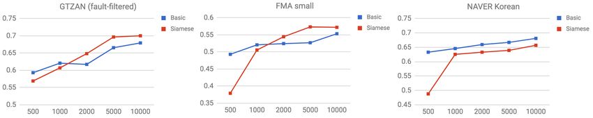
Figure 2. MAP results with regard to different number of artists in the feature models.

   Figure 3. Genre classification accuracy using k-NN with regard to different number of artists in the feature models.

Figure 4. Genre classification accuracy using linear softmax with regard to different number of artists in the feature models.

in the genre classification using k-NN even though they are
based on feature similarity. We dissected the result to see
whether it is related to the cultural difference between the
training data (MSD, mostly Western) and the target data
(the NAVER set, only Korean). Figure 5 shows the de-
tailed classification accuracy for each genre of the NAVER
dataset. In three genres, ‘Trot’,‘K-pop Ballad’ and ‘Kids’
that do not exist in the training dataset, we can see that the
basic model outperforms the Siamese model whereas the
results are opposite in the other genres. This indicates that
the basic model is more robust to unseen genres of music.
On the other hand, the Siamese model slightly over-fits to       Figure 5. The classification results of each genre for the
the training set, although it effectively captures the artist    NAVER dataset with only Korean music.
features.
5.3 Effect of the Number of Artists
                                                                 artists is greater than 1,000. Also, as the number of artists
We further analyze the artist-label models by investigat-        increases, the MAP of the Siamese model consistently
ing how the number of artists in training the DCNN af-           goes up with a slight lower speed whereas that of the ba-
fects the performance. Figure 2, 3 and 4 are the results         sic model saturates at 2,000 or 5,000 artists. On the other
that show similarity-based retrieval (MAP) and genre clas-       hand, the performance gap changes in the two classifica-
sification (accuracy) using k-NN and linear softmax, re-         tion tasks. On the GTZAN dataset, while the basic model
spectively, according to the increasing number of training       is better for 500 and 1,000 artists, the Siamese model
artists. They show that the performance is generally pro-        reverses it for 2,000 and more artists. On the NAVER
portional to the number of artists but the trends are quite      dataset, the basic model is consistently better. On the FMA
different between the two models. In the similarity-based        small, the results are mixed in two classifiers. Again, the
retrieval, the MAP of the Siamese model is significantly         results may be explained by our interpretation of the mod-
higher than that of the basic model when the number of           els in Section 5.2. In summary, the Siamese model seems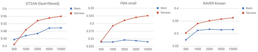
GTZAN
 Models                                            FMA small
                                (fault-filtered)
 2-D CNN [17]                       0.6320             -
 Temporal features [16]             0.6590             -
 Multi-level Multi-scale [20]       0.7200             -
 SVM [7]                                -           0.5482†
 Artist-label Basic model           0.7076          0.5687
 Artist-label Siamese model         0.7203          0.5673

Table 4. Comparison with previous state-of-the-art mod-
els: classification accuracy results. Linear softmax classi-
fier is used and features are extracted from the artist-label
models trained with 10,000 artists. † This result was ob-
tained using the provided code and dataset in [7].
                                                                 Figure 6. Feature visualization by artist. Total 22 artists
                                                                 are used and, among them, 15 artists are represented in
to work better in similarity-based tasks and the basic model     color.
is more robust to different genres of music. In addition,
the Siamese model is more capable of being trained with a
large number of artists.
5.4 Comparison with State-of-the-arts
The effectiveness of artist labels is also supported by com-
parison with previous state-of-the-art models in Table 4.
For this result, we report two artist-label models trained
with 10,000 artists using linear softmax classifier. In this
table, we can see that the proposed models are comparable
to the previous state-of-the-art methods.

                  6. VISUALIZATION
We visualize the extracted feature to provide better insight     Figure 7. Feature visualization by genre. Total 10 genres
on the discriminative power of learned features using artist     from the GTZAN dataset are used.
labels. We used the DCNN trained to classify 5,000 artists
as a feature extractor. After collecting the feature vec-
tors, we embedded them into 2-dimensional vectors using          tween a small subset of the artist labels based on the artist
t-distributed stochastic neighbor embedding (t-SNE).             identity. The last is a model optimized using tag labels
    For artist visualization, we collect a subset of MSD         with the same architecture as the first model. After the
(apart from the training data for the DCNN) from well-           models are trained, we used them as feature extractors and
known artists. Figure 6 shows that artists’ songs are appro-     validated the models on song retrieval and genre classifi-
priately distributed based on genre, vocal style and gender.     cation tasks on three different datasets. Three interesting
For example, artists with similar genre of music are closely     results were found during the experiments. First, the artist-
located and female pop singers are close to each other ex-       label models, particularly the Siamese model, is compa-
cept Maria Callas who is a classical opera singer. Interest-     rable to or outperform the tag-label model. This indicates
ingly, some songs by Michael Jackson are close to female         that the cost-free artist-label is as effective as the expensive
vocals because of his distinctive high-pitched tone.             and possibly noisy tag-label. Second, the Siamese model
    Figure 7 shows the visualization of features extracted       showed the best performances on song retrieval task in all
from the GTZAN dataset. Even though the DCNN was                 datasets tested. This can indicate that the pair-wise rele-
trained to discriminate artist labels, they are well clustered   vance score loss in the Siamese model helps the feature
by genre. Also, we can observe that some genres such             similarity-based search. Third, the use of a large number
as disco, rock and hip-hop are divided into two or more          of artists increases the model performance. This result is
groups that might belong to different sub-genres.                also useful because the artists can be easily increased to a
                                                                 very large number.
      7. CONCLUSION AND FUTURE WORK
                                                                    As future work, we will investigate the artist-label
In this work, we presented the models to learn audio fea-        Siamese model more thoroughly. First, we plan to in-
ture representation using artist labels instead of semantic      vestigate advanced audio model architecture and diverse
labels. We compared two artist-label models and one tag-         loss and pair-wise relevance score functions. Second, the
label model. The first is a basic DCNN consisting of a           model can easily be re-trained using new added artists be-
softmax output layer to predict which artist they belong to      cause the model does not have fixed output layer. This
out of all artists used. The second is a Siamese-style ar-       property will be evaluated using cross-cultural data or us-
chitecture that maximizes the relative similarity score be-      ing extremely small data (i.e. one-shot learning [18]).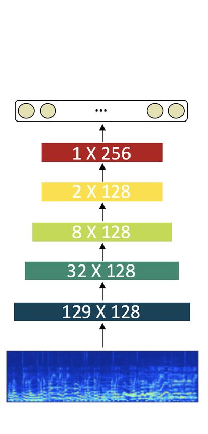
8. ACKNOWLEDGEMENT                                    in neural information processing systems (NIPS),
                                                                     pages 2121–2129, 2013.
 This work was supported by Basic Science Research Pro-
 gram through the National Research Foundation of Korea         [11] Philippe Hamel and Douglas Eck. Learning features
 funded by the Ministry of Science, ICT & Future Planning            from music audio with deep belief networks. In Proc.
 (2015R1C1A1A02036962) and by NAVER Corp.                            of the International Conference on Music Information
                                                                     Retrieval (ISMIR), pages 339–344, 2010.
                    9. REFERENCES
                                                                [12] Mikael Henaff, Kevin Jarrett, Koray Kavukcuoglu, and
 [1] Yoshua Bengio, Aaron Courville, and Pascal Vincent.             Yann LeCun. Unsupervised learning of sparse features
     Representation learning: A review and new perspec-              for scalable audio classification. In Proc. of the Inter-
     tives. IEEE transactions on pattern analysis and ma-            national Conference on Music Information Retrieval
     chine intelligence, 35(8):1798–1828, 2013.                      (ISMIR), pages 681–686, 2011.
 [2] Thierry Bertin-Mahieux, Daniel PW Ellis, Brian Whit-       [13] Po-Sen Huang, Xiaodong He, Jianfeng Gao, Li Deng,
     man, and Paul Lamere. The million song dataset. In              Alex Acero, and Larry Heck. Learning deep structured
     Proc. of the International Society for Music Informa-           semantic models for web search using clickthrough
     tion Retrieval Conference (ISMIR), volume 2, pages              data. In Proc. of the 22nd ACM international confer-
     591–596, 2011.                                                  ence on Conference on information & knowledge man-
 [3] Jane Bromley, Isabelle Guyon, Yann LeCun, Ed-                   agement, pages 2333–2338. ACM, 2013.
     uard Säckinger, and Roopak Shah. Signature verifica-      [14] Eric Humphrey, Juan Bello, and Yann LeCun. Feature
     tion using a “siamese” time delay neural network. In            learning and deep architectures: new directions for mu-
     Advances in Neural Information Processing Systems               sic informatics. Journal of Intelligent Information Sys-
     (NIPS), pages 737–744, 1994.                                    tems, 41(3):461–481, Dec 2013.
 [4] Keunwoo Choi, George Fazekas, and Mark Sandler.
                                                                [15] Sergey Ioffe and Christian Szegedy. Batch normaliza-
     Automatic tagging using deep convolutional neural
                                                                     tion: Accelerating deep network training by reducing
     networks. In Proc. of the International Society for Mu-
                                                                     internal covariate shift. In International Conference on
     sic Information Retrieval Conference (ISMIR), pages
                                                                     Machine Learning (ICML), pages 448–456, 2015.
     805–811, 2016.
                                                                [16] Il-Young Jeong and Kyogu Lee. Learning temporal fea-
 [5] Keunwoo Choi, György Fazekas, Mark Sandler, and
                                                                     tures using a deep neural network and its application
     Kyunghyun Cho. Convolutional recurrent neural net-
                                                                     to music genre classification. In Proc. of the Interna-
     works for music classification. In Proc. of the IEEE In-
                                                                     tional Society for Music Information Retrieval Confer-
     ternational Conference on Acoustics, Speech, and Sig-
                                                                     ence (ISMIR), pages 434–440, 2016.
     nal Processing (ICASSP), pages 2392–2396, 2017.
 [6] Keunwoo Choi, György Fazekas, Mark Sandler, and           [17] Corey Kereliuk, Bob L Sturm, and Jan Larsen. Deep
     Kyunghyun Cho. Transfer learning for music classi-              learning and music adversaries. IEEE Transactions on
     fication and regression tasks. In Proc. of the Interna-         Multimedia, 17(11):2059–2071, 2015.
     tional Conference on Music Information Retrieval (IS-      [18] Gregory Koch, Richard Zemel, and Ruslan Salakhut-
     MIR), pages 141–149, 2017.                                      dinov. Siamese neural networks for one-shot image
 [7] Michaël Defferrard, Kirell Benzi, Pierre Van-                  recognition. In ICML Deep Learning Workshop, vol-
     dergheynst, and Xavier Bresson. Fma: A dataset for              ume 2, 2015.
     music analysis. In Proc. of the International Society
                                                                [19] Honglak Lee, Peter Pham, Yan Largman, and An-
     for Music Information Retrieval Conference (ISMIR),
                                                                     drew Y Ng. Unsupervised feature learning for au-
     pages 316–323, 2017.
                                                                     dio classification using convolutional deep belief net-
 [8] Sander Dieleman and Benjamin Schrauwen. Multi-                  works. In Advances in neural information processing
     scale approaches to music audio feature learning. In            systems (NIPS), pages 1096–1104, 2009.
     International Society for Music Information Retrieval
                                                                [20] Jongpil Lee and Juhan Nam. Multi-level and multi-
     Conference (ISMIR), pages 116–121, 2013.
                                                                     scale feature aggregation using pretrained convolu-
 [9] Sander Dieleman and Benjamin Schrauwen. End-to-                 tional neural networks for music auto-tagging. IEEE
     end learning for music audio. In Proc. of the IEEE In-          Signal Processing Letters, 24(8):1208–1212, 2017.
     ternational Conference on Acoustics, Speech and Sig-
     nal Processing (ICASSP), pages 6964–6968, 2014.            [21] Rui Lu, Kailun Wu, Zhiyao Duan, and Changshui
                                                                     Zhang. Deep ranking: Triplet matchnet for music met-
[10] Andrea Frome, Greg S Corrado, Jon Shlens, Samy                  ric learning. In Proc. of the IEEE International Con-
     Bengio, Jeff Dean, Tomas Mikolov, et al. Devise: A              ference on Acoustics, Speech and Signal Processing
     deep visual-semantic embedding model. In Advances               (ICASSP), pages 121–125, 2017.
[22] Pranay Manocha, Rohan Badlani, Anurag Kumar,
Ankit Shah, Benjamin Elizalde, and Bhiksha Raj.
Content-based representations of audio using siamese
neural networks. In Proc. of the IEEE International
Conference on Acoustics, Speech and Signal Process-
ing (ICASSP), 2018.
[23] Tomas Mikolov, Ilya Sutskever, Kai Chen, Greg S
Corrado, and Jeff Dean. Distributed representations
of words and phrases and their compositionality. In
Advances in neural information processing systems
(NIPS), pages 3111–3119, 2013.
[24] Juhan Nam, Jorge Herrera, Malcolm Slaney, and
Julius O. Smith. Learning sparse feature representa-
tions for music annotation and retrieval. In Proc. of
the International Conference on Music Information Re-
trieval (ISMIR), pages 565–570, 2012.
[25] Jordi Pons, Thomas Lidy, and Xavier Serra. Experi-
menting with musically motivated convolutional neu-
ral networks. In Proc. of the International Workshop
on Content-Based Multimedia Indexing (CBMI), pages
1–6, 2016.
[26] Jan Schlüter and Christian Osendorfer. Music Simi-
larity Estimation with the Mean-Covariance Restricted
Boltzmann Machine. In Proc. of the International Con-
ference on Machine Learning and Applications, pages
118–123, 2011.
[27] Erik M. Schmidt and Youngmoo E. Kim. Learning
emotion-based acoustic features with deep belief net-
works. In Proc. of the IEEE Workshop on Applications
of Signal Processing to Audio and Acoustics (WAS-
PAA), pages 65–68, 2011.
[28] George Tzanetakis and Perry Cook. Musical genre
classification of audio signals. IEEE Transactions on
speech and audio processing, 10(5):293–302, 2002.
[29] Yonatan Vaizman, Brian McFee, and Gert Lanckriet.
Codebook-based audio feature representation for mu-
sic information retrieval. IEEE/ACM Transactions on
Audio, Speech and Language Processing (TASLP),
22(10):1483–1493, 2014.
[30] Jan Wülfing and Martin Riedmiller. Unsupervised
learning of local features for music classification. In
Proc. of the International Society for Music Informa-
tion Retrieval Conference (ISMIR), pages 139–144,
2012.
[31] Chin-Chia Yeh, Li Su, and Yi-Hsuan Yang. Dual-layer
bag-of-frames model for music genre classification. In
Proc. of the IEEE International Conference on Acous-
tics, Speech, and Signal Processing (ICASSP), pages
246–250, 2013.You can also read