GREEN: the new Global Radiation Earth ENvironment model (beta version)
←
→
Page content transcription
If your browser does not render page correctly, please read the page content below
Ann. Geophys., 36, 953–967, 2018
https://doi.org/10.5194/angeo-36-953-2018
© Author(s) 2018. This work is distributed under
the Creative Commons Attribution 4.0 License.

GREEN: the new Global Radiation Earth ENvironment
model (beta version)
Angélica Sicard1 , Daniel Boscher1 , Sébastien Bourdarie1 , Didier Lazaro1 , Denis Standarovski2 , and Robert Ecoffet2
1 ONERA,    The French Aerospace Lab, Toulouse, France
2 CNES,   The French Space Agency, Toulouse, France

Correspondence: Angélica Sicard (angelica.sicard@onera.fr)

Received: 22 March 2018 – Discussion started: 29 March 2018
Revised: 19 June 2018 – Accepted: 19 June 2018 – Published: 4 July 2018

Abstract. GREEN (Global Radiation Earth ENvironment) is           els, primarily due to the covered energy range, but also be-
a new model (in beta version) providing fluxes at any loca-       cause in some regions of space there are discrepancies be-
tion between L∗ = 1 and L∗ = 8, all along the magnetic field      tween the predicted average values and the measurements.
lines, for all local times and for any energy between 1 keV       Moreover, the new US models AE9 and AP9 were devel-
and 10 MeV for electrons and between 1 keV and 800 MeV            oped a few years ago (Ginet et al., 2013). These models are
for protons. This model is composed of global models (AE8         better than AE8 and AP8 in some cases but need to be im-
and AP8, and SPM for low energies) and local models (SLOT         proved in some regions of radiation belts. Therefore, our aim
model, OZONE and IGE-2006 for electrons, and OPAL and             is to develop a radiation belt model, covering a large region
IGP for protons). GREEN is not just a collection of various       of space and energy, from low Earth orbit (LEO) altitudes to
models; it calculates the electron and proton fluxes from the     geostationary Earth orbit (GEO) and above, and from plasma
most relevant existing model for a given energy and location.     to relativistic particles. The aim for the first version of this
Moreover, some existing models can be updated or corrected        new model is to correct the AP8 and AE8 models where they
in GREEN. For examples, a new version of the SLOT model           are deficient or not defined. Ten years ago we developed the
is presented here and has been integrated in GREEN. More-         IGE-2006 model for geostationary orbit electrons (Sicard-
over, a new model of proton flux in geostationary orbit (IGP)     Piet et al., 2008). This model has proven to be more accurate
developed a few years ago is also detailed here and integrated    than AE8 and is used commonly in the industry, covering a
in GREEN. Finally a correction of the AE8 model at high           broad energy range, from 1 keV to 5 MeV. From then, a pro-
energy for L∗ < 2.5 has also been implemented. The inputs         ton model for geostationary orbit, called IGP, was also devel-
of the GREEN model are the coordinates of the points and          oped for material applications and is presented in this paper.
the date (year, month, day, UTC) along an orbit, the particle     These models in geostationary orbit were followed by the
species (electron or proton) and the energies. Then GREEN         OZONE model (Bourdarie et al., 2009), covering a narrower
provides fluxes all along the given orbit, depending on the so-   energy range but the whole outer electron belt; the SLOT
lar cycle and other magnetic parameters such as L∗ , B mirror     model (Sicard-Piet et al., 2014) to assess average electron
and B eq .                                                        values for 2 < L∗ < 4; and finally the OPAL model (Boscher
                                                                  et al., 2014), which provides high-energy proton flux values
                                                                  at low altitudes. As most of these models were developed us-
                                                                  ing more than a solar cycle of measurements – these ones be-
1   Introduction                                                  ing checked, cross-calibrated and filtered – we have no doubt
                                                                  that the obtained averages are more accurate than AP8 and
The well-known NASA AP8 and AE8 models (Sawyer and                AE8 for these particular locations. These local models were
Vette, 1976; Vette, 1991) are commonly used in the satellite      validated along different orbits with independent data sets or
industry to specify the radiation belt environment. Unfortu-      measurements of space environment effects.
nately, there are some limitations in the use of these mod-

Published by Copernicus Publications on behalf of the European Geosciences Union.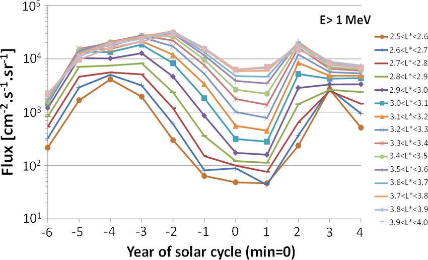
954                        A. Sicard et al.: GREEN: the new Global Radiation Earth ENvironment model (beta version)

Figure 1. Input and output parameters of the GREEN model.

   Obviously, the ideal would be to develop a unified global      (Boscher et al., 2014) and SPM (Ginet et al., 2013). The sec-
model across many L∗ and energies rather than combining           ond step was to define a 3-D grid in energy (Ec), B local /B eq
“submodels”. However, radiation belts are made of several         (with B local the local magnetic field and B eq the equatorial
regions with different dynamics and several populations (low      magnetic field) and L∗ . This grid represents the global archi-
energies and high energies) with different behavior. So it is     tecture of GREEN. This 3-D grid (Ec, B local /B eq , L) is the
easier to develop local models for each region and each en-       same as the one used for the physical model Salammbô (Her-
ergy range.                                                       rera et al., 2016, and references therein) with 133 steps in L∗
   In order to develop a new global model, called GREEN           (between L∗ = 1 and L∗ = 8), 133 steps in B local /B eq and
(Global Radiation Earth ENvironment), with GREEN-e for            49 steps in energy and has not been chosen randomly. After
electrons and GREEN-p for protons, we will use a cache file       verification, this grid allows the results of the most binding
system to switch between models, in order to obtain the most      model (for example OPAL) to be reproduced as best as pos-
reliable value at each location in space and each energy point.   sible. Obviously the energy grid is different for GREEN-e
Of course, the way the model is developed is well suited to       and GREEN-p. Then, fluxes from each model integrated in
future enhancement with new models developed locally or           GREEN are calculated on this 3-D grid. Taking into account
under international partnerships. The first beta version of the   that some local models that compose GREEN give only flux
GREEN model is presented in this paper.                           integrated in energy, only this kind of flux is provided by
                                                                  GREEN (cm−2 s−1 ). Finally, a priority order of the different
                                                                  models is established according to space location and energy
2     Development of the model                                    to provide the most reliable value of flux. The last step is
                                                                  to calculate flux for a given energy and a given location by
2.1    Main principles                                            interpolating in the 3-D grid of the most reliable model.
                                                                     Figure 1 is a scheme describing all the input parame-
GREEN is a new model composed of different global and lo-         ters, the core of the model and all the output parameters
cal models. The first step of the development was to define a     of GREEN. One of the features of GREEN is that it pro-
list of the most relevant models in the case of electrons and     vides fluxes depending on the year of the solar cycle and not
another one for protons. These two lists can be expanded and      just two states as in the case of AE8 (AE8 MIN and AE8
modified at any time. GREEN-e is composed of AE8 (Vette,          MAX). Moreover, when it is possible, GREEN also provides
1991), the SLOT model (Sicard-Piet et al., 2014), OZONE           the maximum envelope of the mean flux, depending also on
(Bourdarie et al., 2009), IGE-2006 (Sicard-Piet et al., 2008)     the year of the solar cycle, due to the variation from one solar
and SPM for the lower energies (Ginet et al., 2013). GREEN-
p is composed of AP8 (Sawyer and Vette, 1976), OPAL

Ann. Geophys., 36, 953–967, 2018                                                          www.ann-geophys.net/36/953/2018/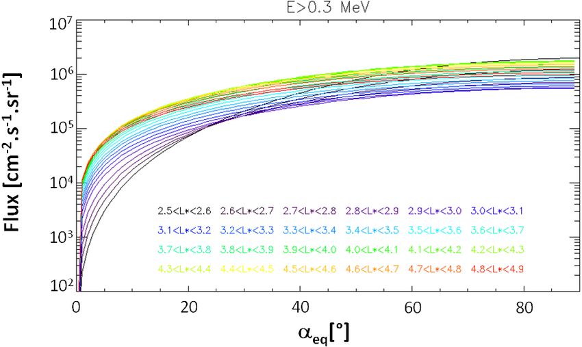
A. Sicard et al.: GREEN: the new Global Radiation Earth ENvironment model (beta version)                                        955

Figure 2. Energy and L coverage of the different models integrated in GREEN-e.

cycle to another (as explained in detail for IGE-2006; Sicard-       use a corrected version of AE8. Indeed, in a previous study,
Piet et al., 2008).                                                  Boscher at al. (2018) showed that high-energy electron fluxes
                                                                     (greater than a few hundred kiloelectron volts) predicted by
2.2     GREEN-e                                                      AE8 are overestimated in the region for L∗ < 2.5. It is diffi-
                                                                     cult to estimate the error made by AE8, but this study aims
In this section, the electron part of GREEN, GREEN-e, is de-         at showing that in this region and for high energy the phys-
scribed in detail. Figure 2 represents energy and L coverage         ical model Salammbô provides electron fluxes in agreement
of the different models integrated in GREEN-e. It is impor-          with in situ measurements. Thus, in this version of GREEN-e
tant to keep in mind that most of the models are defined in          model, AE8 fluxes have been corrected, that is to say, divided
terms of L∗ calculated with International Geomagnetic Ref-           by a given factor, calculated using the Salammbô model. The
erence Field (IGRF) + Olson–Pfitzer magnetic field models,           Salammbô model is not perfect everywhere, but it has been
except AE8. Indeed, when AE8 is used, the L parameter must           proven that the decrease of electron flux with energy is good
be calculated with the Jensen and Cain magnetic field model          (Boscher et al., 2018). Thus, when electron fluxes from AE8
(Vette, 1991).                                                       are higher than those provided by Salammbô, they are di-
                                                                     vided by the ratio between the both, up to a factor 100, in
2.2.1    AE8 and SPM                                                 order to limit the correction (Fig. 3). This correction is not
                                                                     perfect but does allow better estimation of high-energy elec-
As mentioned in Fig. 2, AE8 and SPM are used by default.             tron flux in the region L∗ < 2.5.
This is the case for the SPM model at low energy (< 30 keV)
except in geostationary orbit when IGE-2006 is preferred and         2.2.2   SLOT model
for AE8 at higher energy (> 30 keV) outside the coverage of
the SLOT model, OZONE and IGE-2006. SPM is a model                   Figure 2 shows also that the SLOT model is available from
with no solar cycle dependence; thus electron fluxes result-         L∗ = 2.5 to L∗ = 5 and for energies from 100 keV to 3 MeV.
ing from this model are considered constant throughout the           The SLOT model developed in 2013 (Sicard-Piet et al., 2014)
solar cycle. For AE8, two versions exist: AE8 MAX for the            was a model that reflects the mean flux at each point along
solar maximum and AE8 MIN for the solar minimum. It is               the magnetic field lines. This first version has been updated
common to consider a full solar cycle of 11 years with 4 years       in 2017 and is described here. As explained in a previous
of solar minimum (2 years before the minimum and 2 years             paper (Sicard-Piet et al., 2014), the SLOT model is based
after) and 7 years of solar maximum. Thus, in GREEN, when            on the correlation between the flux dynamics in LEO orbit
AE8 is the preferred model, the appropriate version of AE8           with NOAA-POES (Polar Operational Environmental Satel-
(MIN or MAX) is taken according to the year chosen by the            lites) data and the flux all along the magnetic field line. The
user.                                                                first change in the model is its spatial extension: the upper
   The inner zone of electron radiation belts is a region in         spatial limit of the SLOT model is now L∗ = 5 as opposed
which interest has grown in recent years thanks to data from         to L∗ = 4 before. Then, taking into account new measure-
the Van Allen Probes (Li et al., 2015; Claudepierre et al.,          ments such as those from the Van Allen Probes (MagEIS),
2017). As mentioned in this figure, for L < 2.5 and energy           correlation factors all along the magnetic field line have been
greater than a few hundred kiloelectron volts, we choose to          recalculated, between L∗ = 2.5 and L∗ = 5. An example of

www.ann-geophys.net/36/953/2018/                                                              Ann. Geophys., 36, 953–967, 2018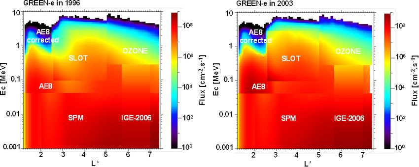
956                        A. Sicard et al.: GREEN: the new Global Radiation Earth ENvironment model (beta version)

Figure 3. Electron fluxes provided by Salammbô in blue (average of years during solar minimum), by AE8 MIN in red and AE8 MIN
corrected in green at L = 2.

Figure 4. Example of correlation between NOAA-POES and Van Allen Probe-A flux for electrons > 0.3 MeV and for L∗ between 3.7 and
3.8.

the correlation between NOAA-POES data and Van Allen                 The most significant change in this new version of the
Probe-A measurements is plotted in Fig. 4 for electrons with      SLOT model is the dependence of fluxes on the solar cycle.
energy > 0.3 MeV and for L∗ between 3.7 and 3.8. This kind        In order to have dependence on the solar cycle in GREEN-e,
of correlation is made with all data used in the model and        we have to study in detail the dynamics of the measurements
listed in Sicard-Piet et al. (2014) plus the Van Allen Probes.    from all NOAA-POES spacecraft. As an example of this so-
As explained by Sicard-Piet et al. (2014), these correlation      lar cycle dependence, > 300 keV electron fluxes vs. time from
factors are multiplied with the NOAA-POES data in order           all NOAA-POES data is plotted in Fig. 6. This figure shows
to obtain mean electron fluxes between > 0.1 and > 3 MeV          clearly a correlation between the dynamics of NOAA-POES
along all magnetic field lines between L∗ = 2.5 and L∗ = 5        electron fluxes and the solar cycle (F10.7). The dynamics
(Fig. 5). An equatorial pitch angle distribution shape based      have been studied for four energy channels: > 0.1, > 0.3, > 1
on a sine function is assumed and constrained by data all         and > 3 MeV.
along the magnetic field lines between L∗ = 2.5 and L∗ = 5           Then, the flux dynamics over time between 1978 and 2015
(Fig. 5).                                                         have been represented in the 11 years of the solar cycle, from
                                                                  year −6 to year 4, with year 0 being the solar minimum.

Ann. Geophys., 36, 953–967, 2018                                                          www.ann-geophys.net/36/953/2018/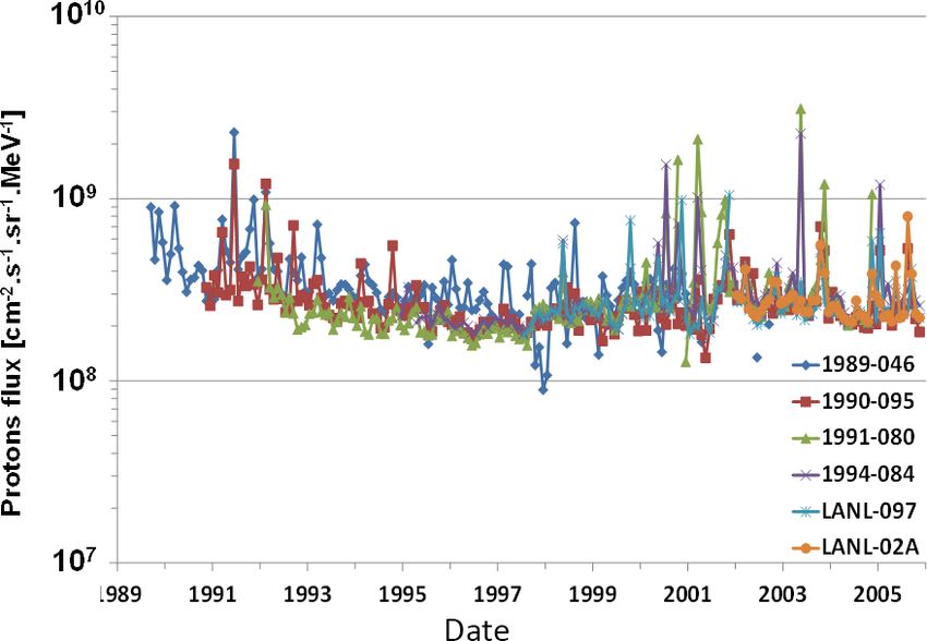
A. Sicard et al.: GREEN: the new Global Radiation Earth ENvironment model (beta version) 957
Figure 5. Electron fluxes along magnetic field lines (90◦ corresponds to the Equator) for energy > 0.3 MeV and for all L∗ intervals of the
SLOT model (in color).
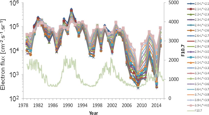
Figure 6. Electron > 300 keV fluxes vs. time (1978–2015) from all NOAA-POES data for each L∗ interval defined in the SLOT model. F10.7
is also represented in green.
The fluxes vs. year of the solar cycle in NOAA-POES or- 2006 results; consequently OZONE will be used for energies
bit for electrons > 1 MeV and for each L∗ interval is plotted > 300 keV in GEO orbit. The version of OZONE developed
in Fig. 7. This modulation with the solar cycle has been de- in 2009 (Bourdarie et al., 2009) was already dependent on the
fined in LEO orbit for the four energy channels of the SLOT solar cycle, so the model was not modified before integration
model and has been applied to the mean flux all along the in GREEN-e.
magnetic field lines, from low altitude to the Equator.
Finally, in order to take into account the modulation of flux 2.2.4 IGE-2006 model
from one solar cycle to another, this new version of the SLOT
model provides mean flux for a given year of the solar cycle IGE-2006 is a specification model developed exclusively for
as well as the maximum flux of the three solar cycles used in geostationary orbit (Sicard-Piet et al., 2008). This orbit is at a
the model for this given year. fixed altitude but is represented by a large L∗ range, between
Thus, the new version of the SLOT model provides elec- 5.7 and 7.1. As explained in Sicard-Piet et al. (2008), fluxes
tron fluxes from 0.1 to 3 MeV for all altitudes with L∗ be- provided by IGE-2006 come from averaged fluxes measured
tween 2.5 and 5 with a dependence on the solar cycle. by all available Los Alamos National Laboratory (LANL)
spacecraft. In this version of GREEN-e, fluxes will be con-
2.2.3 OZONE model sidered as a constant in this L∗ range. IGE-2006 is solar cycle
dependent, so the model was not modified before integration
OZONE is valid for L∗ > 4 and for energies greater than in GREEN-e.
300 keV. In geostationary orbit, OZONE agrees with IGE-
www.ann-geophys.net/36/953/2018/ Ann. Geophys., 36, 953–967, 2018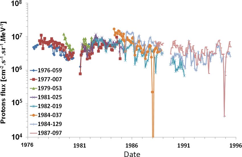
958                         A. Sicard et al.: GREEN: the new Global Radiation Earth ENvironment model (beta version)

Figure 7. Electron > 1 MeV fluxes vs. year of the solar cycle from all NOAA-POES data for each L∗ interval defined in the SLOT model.

Figure 8. Energy and L coverage of the different models integrated in GREEN-p.

2.3     GREEN-p                                                       sion of OPAL has been developed at ONERA, using ICARE-
                                                                      NG measurements on board Jason-2 and Jason-3 (Boscher et
In this section, the proton part of GREEN, GREEN-p, is de-            al., 2011). Now OPAL-v2 provides proton fluxes for energy
scribed in detail. Figure 8 represents energy and L coverage          between 80 and 800 MeV up to the orbit of Jason spacecraft
of the different models integrated in GREEN-p. It is impor-           (1336 km). It is important to keep in mind that input param-
tant to keep in mind that most of the models are defined              eters of OPAL are the radio flux F10.7 of the Sun and the
in terms of L∗ calculated with IGRF + Olson–Pfitzer (Ol-              magnetic field of the given year. As OPAL depends on the ra-
son and Pfitzer, 1977) magnetic field models, except AP8.             dio flux F10.7, an input of OPAL is the date. So, for a given
Indeed, when AP8 is used, the L parameter must be calcu-              date chosen by the user in the past, the real F10.7 value is
lated with the Jensen and Cain magnetic field model for AP8           used to calculate proton fluxes. But for a given date in the
MIN and the Goddard Space Flight Center (GSFC) model                  future, it is not so easy because the F10.7 value is unknown.
for AP8 MAX (Sawyer and Vette, 1976).                                 Consequently, a statistical study has been done on F10.7 val-
                                                                      ues from 1947 to now in order to define a mean F10.7 value
2.3.1    OPAL                                                         for each of the 11 years of a solar cycle. Thus, for a given
                                                                      date chosen by the user in the future, the year of the solar
The first version of OPAL was a model valid for protons
                                                                      cycle is predicted (from year −6 to year +4, with 0 being the
> 80 MeV and for altitude lower than 800 km, depending on
                                                                      year of the minimum), according to which the corresponding
the solar cycle (Boscher et al., 2014). This year, a new ver-

Ann. Geophys., 36, 953–967, 2018                                                               www.ann-geophys.net/36/953/2018/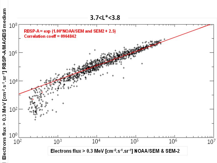
A. Sicard et al.: GREEN: the new Global Radiation Earth ENvironment model (beta version)                                        959

Figure 9. Example of proton flux spectrum (cm−2 s−1 sr−1 ) resulting from OPAL-V2 (in blue) and AP8 MIN (in green).

mean F10.7 value is used in OPAL to calculate proton fluxes.        time; it drifted. This drift is compensated for over time, but
Moreover, added to the mean proton fluxes, OPAL provides            after several years it is impossible to measure the highest
an upper envelope considering the variation from one solar          energies anymore (typically after 10 years, it is impossible
cycle to another. Taking into account that high-energy proton       to obtain measurements above 10 keV). For the development
fluxes are anticorrelated with F10.7 values, this upper enve-       of a proton specification model, data between 1 and 32 keV
lope is calculated using the minimum F10.7 value measured           have been used. Fluxes below 1 keV have not been used,
since 1947 for each year of the solar cycle.                        due to uncertainties in the spacecraft potential determina-
   Figure 9 represents an example of a proton flux spec-            tion. Thus, we determined monthly averages of the proton
trum (cm−2 s−1 sr−1 ) at L∗ = 1.3 near the magnetic equa-           flux for each satellite. These monthly averages were made
tor (αeq = 85.125◦ ) resulting from OPAL-V2 (in blue) and           in order to analyze possible solar cycle or seasonal effects
AP8 MIN (in green). We can observe that, for this L∗ value,         (linked to the magnetic field or to its activity). An exam-
fluxes from OPAL-V2 are slightly higher than those from             ple is given for the 1 keV protons in Fig. 10. Some points
AP8 MIN. This new version of OPAL has been integrated               as high as 2.3 × 10⁹ MeV−1 cm−2 s−1 sr−1 observed in June
in GREEN-p.                                                         1991 could be due to the effect of magnetic activity, a par-
                                                                    ticular contamination during that period or a (or several) bad
2.3.2   IGP                                                         point(s). Apart from these, no seasonal effect is observed in
                                                                    the flux curve; if there is a solar cycle effect, it is very low.
On board the Los Alamos National Laboratory satellites,             As the flux does not vary with time, an average spectrum was
from July 1976 (launch of the satellite: 1976-059) to June          deduced from all the measurements, taking into account the
1995 (end of the measurements on board: 1984-129 and                number of points for each satellite.
1987-097), there was a detector named CPA (Charged Par-
ticle Analyzer), which covered the energy range 80 keV–             CPA measurements
300 MeV (Higbie et al., 1978; Baker et al., 1979). To cover
a larger energy range, we also used the measurements of the         The CPA instrument is in fact made of two different instru-
MPA (Magnetospheric Plasma Analyzer) detector on board              ments: CPA-LoP and CPA-HiP, which respond respectively
LANL satellites being launched between September 1989               to protons in the range 73–512 keV and 400 keV–300 MeV.
(launch of the satellite: 1989-046) and November 1995 (Mc-          The measurements are also globally of high quality. The time
Comas et al., 1993). These measurements cover roughly the           resolution of the instrument is 10 s, which means that the
energy range, 0.1–38 keV.                                           number of points is much higher. A monthly average for each
                                                                    channel was produced. An example of this average is plotted
MPA measurements                                                    in Fig. 11 for 80 keV protons for each available LANL space-
                                                                    craft. From that figure, it appears that there is no seasonal
MPA measurements are globally of good quality. The tem-             variation in the 80 keV proton flux; if there is a solar cycle
poral resolution is 86 s most of the time, but it can be dou-       one, it should be small in the range covered by CPA-LoP (less
bled (172 s) for short periods of time. The detector aged with      than a factor of 2). We must note in this figure a few low flux

www.ann-geophys.net/36/953/2018/                                                              Ann. Geophys., 36, 953–967, 2018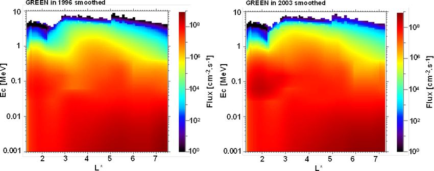
960                         A. Sicard et al.: GREEN: the new Global Radiation Earth ENvironment model (beta version)

Figure 10. Monthly average 1 keV proton flux measured in GEO by the detector MPA on board the different LANL satellites.

Figure 11. Monthly average 80 keV proton flux measured in GEO by the detector CPA-LoP on board the different LANL satellites.

values which lie below the general tendency of the curve; it         erages from the full time period and all spacecraft. Though a
is suspected that they are due to gain switches for that partic-     gap exists between the two instruments, it appears that both
ular channel and that satellite. We have not removed them, as        parts of the spectrum are consistent: at low energy the spec-
the total average is not affected by these points.                   trum is very flat; it falls very quickly for energies greater than
   As for MPA, a global average of all the points was per-           50 keV. We also compared in this figure the obtained spec-
formed, in order to obtain a global spectrum of protons from         trum with AP8 (for longitude 0◦ , AP8 MAX and MIN being
1 keV up to 1 MeV in geostationary orbit. Above 1 MeV, data          equal in this region) (Sawyer and Vette, 1976). For unidirec-
were not used because of the contamination by protons from           tional flux comparison, we divided the AP8 flux by 4π , the
solar flares.                                                        environment being nearly isotropic in geosynchronous orbit
                                                                     for trapped particles. We can see that the obtained spectrum
IGP model                                                            is nearly consistent with AP8. In fact, near 1MeV, the main
                                                                     problem is distinguishing trapped particles from untrapped
Combining the part of the spectrum from MPA and CPA up               ones (solar protons and cosmic rays). That may explain part
to around 1 MeV leads to Fig. 12. The average fluxes are             of the difference. Globally, while the obtained spectrum is
plotted, together with an error bar which corresponds to the         nearly a power law, AP8 is more an exponential law, with
maximum and minimum values obtained in the monthly av-               characteristic energy around 100 keV.

Ann. Geophys., 36, 953–967, 2018                                                              www.ann-geophys.net/36/953/2018/
A. Sicard et al.: GREEN: the new Global Radiation Earth ENvironment model (beta version) 961
Figure 12. Total spectrum of trapped protons deduced from MPA and CPA measurements on board different LANL satellites and from the
model. Fluxes from AP8 and AP9 are provided for comparison.
We tried to determine an empirical formula with all the av- ing to the west, only cosmic rays and solar protons coming
erage flux values. For the high-energy part, we used a kappa from outside the magnetosphere are observed. That is why
function with 9 keV characteristic energy and = 5.45, not far in our analysis no points were extracted for E > 1.14 MeV.
from what was obtained by Christon et al. (1991) in the The model just gives an extrapolation (reasonable as a power
plasma sheet. An exponential part (with 2 keV characteris- law). It is really difficult to validate the IGP model with other
tic energy) was added at low energy to fit the total spectrum: data, because good proton data are extremely rare in GEO
−6.45 orbit, due to contamination by electrons measurements and
E
flux = 4 × 10⁸ exp(−E/0.002) + 7 × 10¹⁰ E 1 + , solar protons.
5.45x0.009
where E is the energy in megaelectron volts (MeV) and the 3 Results and validation
flux in MeV−1 cm−2 s−1 sr−1 .
The model result is compared to the average spectrum in Once each of the local models has been integrated into
Fig. 12. This spectrum is very useful for deducing surface GREEN, we are able to calculate fluxes at any location be-
material degradation for satellites in geostationary orbit. It tween L∗ = 1 and L∗ = 8 all along the magnetic field lines
also can be used for dynamic physical modeling of the radi- and for any energy between 1 keV and 10 MeV for electrons
ation belt proton to set a boundary condition. and between 1 keV and 800 MeV for protons. Figure 13 gives
This model is compared to the NASA AP9-SPM one examples of electron fluxes provided by the GREEN-e model
(Ginet et al., 2013; Roth et al., 2014) also in Fig. 12. The in 1996 (solar minimum) and in 2003 (solar maximum) vs.
NASA AP8 model was limited to energies greater than L∗ and energy at the Equator. The different models used are
100 keV. In geostationary orbit, the low-energy part comes also mentioned on the plot. This figure shows clearly the in-
from the same measurements we used: the MPA detector fluence of the solar cycle on the electron flux, particularly in
on board the LANL spacecraft and the two models are very the Slot region where fluxes are higher during solar maxi-
close (the difference can be due to the interpolation used be- mum. Moreover, we can note that discontinuities exist at the
tween channels). In AP9-SPM, the obtained spectrum is ex- interface of the different models and have to be removed or
trapolated to around 100 keV, but it is possible that our way to at least smoothed in the future versions of GREEN-e. There
connect the two parts of the model has to be improved. With are several ways to attenuate these discontinuities. The first
AP9-SPM, the two parts of the spectrum do not match. Ob- one is to apply a simple smooth function to the 3-D grid of
viously, there is a discontinuity at around 100 keV. At higher GREEN. An example of results obtained with this kind of
energy levels, the spectra from AP8 and AP9 are not too dif- smooth function is represented in Fig. 14. This figure shows
ferent, up to around 500 keV. Above this value, AP9 exceeds that the discontinuities are clearly attenuated but the error
AP8 by a growing factor. The main problem for such energies on the electron flux can remain significant at the interface of
is distinguishing trapped and untrapped particles in the mea- the models. The second method would be to apply a more
surements. We know from magnetospheric shielding calcula- complex smooth function, for example by using our phys-
tions that for this energy range both particles can be observed ical model, Salammbô. But the way to do that needs to be
depending on the viewing direction. Looking to the east, well thought out and defined. The third method, the best but
trapped particles from the radiation belts are observed; look- the hardest, would be to improve the different models close
www.ann-geophys.net/36/953/2018/ Ann. Geophys., 36, 953–967, 2018962 A. Sicard et al.: GREEN: the new Global Radiation Earth ENvironment model (beta version) Figure 13. Electron fluxes vs. L∗ and energy in 1996 and 2003 provided by the GREEN-e model. Figure 14. Electron fluxes vs. L∗ and energy in 1996 and 2003 provided by the GREEN-e model with a simple smooth function. to their boundaries, with new measurements for example. If vided by the GREEN-e model are coherent with those result- each model on one side and the other of an interface provides ing from the MEO-V2 model: equal or slightly higher than a flux closer to a real flux, discontinuities will be removed. mean MEO-V2 fluxes and lower than upper envelope fluxes. The different methods of attenuating discontinuities will be Fluxes from GREEN are also coherent with AE8 and AE9, investigated in detail in the future versions of the GREEN except for energies greater than 5 MeV, where AE9 provides model. electron fluxes higher than GREEN and AE8. Now that the results of GREEN-e have been presented, it In order to validate fluxes in other orbits, a comparison is important to validate them. For the validation, results from between GREEN-e results and NOAA-POES measurements GREEN will be presented without any smooth functions. is done in LEO orbit. Figure 16 represents (i) mean electron The first validation is done in medium Earth orbit (MEO) fluxes between 1999 and 2010 from NOAA-POES measure- by comparing electron fluxes provided by GREEN-e and by ments (in dashed lines) for several energy channels (> 30, other models: the MEO-V2 model (Sicard-Piet et al., 2006), > 100, > 300 keV, > 1 and > 3 MeV) and fluxes from GREEN- AE8, and AE9 and AP9 (v1.5). MEO-v2 model is not used e, calculated based on a full solar cycle, and (ii) electron in GREEN-e and is a good way to validate it. Figure 15 rep- fluxes resulting from the AE9 v1.5 mean. This figure shows resents the electron spectrum from GREEN-e in blue, from that beyond L∗ = 2.5 fluxes resulting from GREEN-e are the MEO-V2 model in red for the mean flux and in green for in agreement with NOAA-POES data, with less than a fac- the upper envelope, and from AE8 in purple for a whole solar tor 3 between the two, particularly in the L range of the cycle. Results from AE9 and AP9 (v1.5 mean) are also plot- SLOT model (2.5 < L∗ < 5), which is based on these data. ted in light blue. This figure shows that electron fluxes pro- At high energy (> 3 MeV) for L∗ > 6, POES data seem to Ann. Geophys., 36, 953–967, 2018 www.ann-geophys.net/36/953/2018/
A. Sicard et al.: GREEN: the new Global Radiation Earth ENvironment model (beta version)                                          963

Figure 15. Electron spectrum from GREEN-e (in blue) in a whole solar cycle compared to the mean (in red) and upper (in green) flux
provided by the MEO-V2 model.

Figure 16. (a) Mean electron fluxes in LEO orbit between 1999 and 2010 from NOAA-POES measurements (in dashed lines) and from one
solar cycle in GREEN-e (in full lines) for several energy channels. (b) Electron fluxes in LEO orbit (820 km, 98◦ ) from AE9 v1.5 mean.

reach the background of the instrument, probably due to cos-          is not usual. It is important to keep in mind that for low
mic particle measurements, while fluxes from the GREEN-e              energy (∼ 30 keV), electron fluxes in GREEN-e come from
model continue to decline while L∗ increases. We can note             AE8, while fluxes for higher energies come from the SLOT
that for low energy (∼ 30 keV) there is a big difference be-          model and OZONE. This energy channel (∼ 30 keV) would
tween GREEN-e and NOAA-POES measurements and that                     be a track of improvement of GREEN. Moreover, fluxes be-
for some L∗ values this flux is lower than > 100 keV, which           low L∗ = 2.5 are not plotted in the figure because it is well

www.ann-geophys.net/36/953/2018/                                                                Ann. Geophys., 36, 953–967, 2018
964                        A. Sicard et al.: GREEN: the new Global Radiation Earth ENvironment model (beta version)

Figure 17. Mean electron fluxes in Jason-2 orbit between 2009 and 2015 from GREEN-e (in full line), Jason-2 measurements (in dashed
line) and AE9 mean v1.5 (dash-dotted line) for E > 2.02 MeV electrons.

known that NOAA-POES data are contaminated by very high                In order to illustrate the reason for this difference between
energy protons at low L∗ values (Evans and Greer, 2000). We         Jason-2 measurements and GREEN and AE9 results, Fig. 18
can also note that there are significant differences between        has been plotted. It is the same figure as Fig. 16 but not dur-
GREEN-e and AE9 above L∗ = 4.5. In LEO orbit, the higher            ing the same period of time: 2009 to 2015 for Fig. 18 as op-
the value of L∗ , the further away from the Equator and the         posed to 1999 to 2010 for Fig. 16. This figure shows that the
more the electron fluxes differ between AE9 and GREEN.              comparison between in situ measurements and GREEN re-
So it seems that, near the Equator, GREEN and AE9 are co-           sults depends on the period of time. If the period of time of
herent, but it is no longer the case at the end of the magnetic     in situ measurements is long enough (several solar cycles) or
field lines for low pitch angles.                                   is representative of a mean flux, data will easily be compared
   The same kind of comparison has been made between                to GREEN results. On the other hand, if the period of time
GREEN-e results and Jason-2 data for E > 2.02 MeV elec-             of in situ measurements is too short compared to a solar cy-
trons for L∗ > 2.5 between 2009 and 2015 and is plotted in          cle or is during a very quiet solar cycle, which is the case for
Fig. 17. The period 2009 to 2015 corresponds to years 0, 1,         Jason-2 measurements, comparison with GREEN flux will
2, 3, 4, −5 and −6 of the solar cycle (0 is the year of the         not be so easy. So the difference of flux at L∗ < 3.5 between
minimum). In Fig. 17, fluxes are an average of results from         GREEN-e and Jason-2 data in Fig. 17 or between GREEN-e
GREEN-e for these years of the solar cycle. Electron fluxes         and NOAA-POES data in Fig. 18 is clearly due to the period
from AE9 (mean v1.5) are also plotted. This graph shows             of time, which corresponds to very quiet years, not represen-
first that there is a discontinuity in the GREEN-e model            tative of a mean solar cycle.
at L∗ = 5, at the interface between the SLOT model and                 Concerning the model GREEN-p, it is much less finalized
OZONE. It is clear that some efforts must be made to remove         than the electron version GREEN-e because only the OPAL
this kind of discontinuity in the next version of GREEN.            model, which has a narrow spatial coverage, has been im-
We can also mention the significant difference between AE9          plemented in addition to AP8 and SPM. It is really difficult
and GREEN at L∗ > 4.5 as in the case of Fig. 16. However,           to measure protons of energy around megaelectron volts in
what we want to highlight with this plot is the difference be-      the radiation belts because of the predominant presence of
tween GREEN-e results and Jason-2 measurements for low              the electrons which very often contaminate the data. Thus,
L∗ values (L∗ < 3.5). Electron flux measured by Jason-2 at          due to a lack of good-quality data in sufficient numbers, it is
this energy level is much lower than the one provided by            difficult to develop a model of protons for energies around
GREEN and AE9 in this region, while Fig. 16 showed a very           megaelectron volts. Some efforts will be made in the near fu-
good correlation between GREEN, AE9 and NOAA mea-                   ture to improve the modeling of megaelectron-volt protons in
surements in the same region (L∗ < 3.5). Why was there an           GREEN-p and compare the results with measurements from
agreement between the results of GREEN and NOAA that no             GPS or THEMIS for example.
longer appears with the Jason-2 measurements? Is this due to           However, we can still present an example of results from
the difference of altitude between the two spacecraft (800 km       GREEN-p and compare them to AP8, even if only OPAL-V2
for NOAA and 1336 km for Jason-2)?                                  is integrated in the global model. Figure 19 represents pro-
                                                                    ton fluxes vs. L∗ resulting from GREEN-p and AP8 MIN

Ann. Geophys., 36, 953–967, 2018                                                            www.ann-geophys.net/36/953/2018/
A. Sicard et al.: GREEN: the new Global Radiation Earth ENvironment model (beta version) 965
Figure 18. Mean electron fluxes in LEO orbit between 2009 and 2015 from NOAA-POES measurements (in dashed lines) and from GREEN-
e (in full lines) for several energy channels.
Figure 19. Proton fluxes vs. L∗ resulting from GREEN-p and AP8 MIN at two magnetic latitudes corresponding to αeq = 90◦ and αeq = 50◦
for E > 80 MeV protons.
at two magnetic latitudes corresponding to αeq = 90◦ and isting models with also some improvements, especially at
αeq = 50◦ , for E > 80 MeV protons. This figure shows that high energy and low L∗ values where the AE8 model has
fluxes from GREEN-p come from OPAL-V2 up to L∗ = 1.3 been corrected, or in the Slot region with the new version of
for αeq = 90◦ and up to L∗ = 1.5 for αeq = 50◦ and from AP8 the SLOT model. Obviously, despite our efforts, some dis-
beyond. At very low L∗ , when AP8 and OPAL-V2 are avail- continuities exist at the interface of the models but will be
able, some small differences appear in the flux. At αeq = 50◦ removed or at least smoothed in the next versions. The ma-
fluxes for GREEN-p are slightly lower than AP8 MIN. jor advantage of GREEN is the dependence of fluxes on the
solar cycle. Most of models included in GREEN are solar
4 Discussion and conclusions cycle dependent, which allows it to have a better estimation
of fluxes according to the duration of the mission vs. solar
GREEN (Global Radiation Earth ENvironment) is a new cycle. Indeed, fluxes provided by the GREEN model are dif-
model providing fluxes at any location between L∗ = 1 and ferent for each of the 11 years of the solar cycle. Concerninga
L∗ = 8 all along the magnetic field lines and for any en- GREEN-p, which is less finalized than GREEN-e, the major
ergy between 1 keV and 10 MeV for electrons and between advantage is in geostationary orbit with the IGP model and
1 keV and 800 MeV for protons. This model is composed at low altitude when OPAL is available, with not only the de-
of global models (AE8 and AP8, and SPM) as well as lo- pendence on the year of the solar cycle but also directly the
cal models (SLOT model, OZONE and IGE-2006 for elec- dependence on the radio flux F10.7 of the Sun and the mag-
trons, and OPAL and IGP for protons). These local mod- netic field of the given year. In the next versions of GREEN-
els are used when they are more relevant than AE8 AP8 or p, future studies will allow the magnetic field to be predicted
SPM. Thus, this version of GREEN is a patchwork of ex-
www.ann-geophys.net/36/953/2018/ Ann. Geophys., 36, 953–967, 2018966 A. Sicard et al.: GREEN: the new Global Radiation Earth ENvironment model (beta version)
for up to several decades and thus will have a better estima- Belt Specification Model, IEEE T. Nucl. Sci., 56, 2251–2257,
tion of the proton fluxes at low altitude. Moreover, in the near https://doi.org/10.1109/TNS.2009.2014844, 2009.
future, some efforts will be made to try to extend the OPAL Christon, S. P., Williams, D. J., Mitchell, M. G., Huang, C. Y., and
model to higher altitude and lower energy by using all the Franck, L. A.: Spectral characteristics of plasma sheet ion and
available good-quality data (GPS or THEMIS for example), electron populations during disturbed geomagnetic conditions, J.
Geophys. Res., 96, 1–22, 1991.
even if we know it will be a hard task.
Claudepierre, S. G., O’Brien, T. P., Fennell, J. F., Blake, J. B., Clem-
Another advantage of GREEN is that it is easy to upgrade. mons, J. H., Looper, M. D., Mazur J. E., Roeder J. L.,Turner,
Indeed, a cache file system allows switching between mod- D. L., Reeves, G. D., and Spence, H. E.: The hidden dynam-
els, in order to obtain the most reliable value at each location ics of relativistic electrons (0.7–1.5 MeV) in the inner zone and
in space and each energy point. Thus, the way the model is slot region, J. Geophys. Res. Space Physics, 122, 3127–3144,
developed is well suited to adding new local developments https://doi.org/10.1002/2016JA023719, 2017.
or to including international partnership. Evans, D. and Greer, M. S.: Polar Orbiting Environmental Satellite
Finally a perspective of GREEN, other than the improve- Space Environment Monitor – 2: Instrument Descriptions and
ment of flux accuracy, would be to develop a special “worst- Archive Data Documentation, NOAA Technical Memorandum,
case” version of GREEN in order to adapt it to space industry 2000.
user needs in the case of short-term missions, typically a few Ginet, G. P., O’Brien, T. P., Huston, S. L., Johnston, W. R., Guild, T.
B., Friedel, R., Lindstrom, C. D., Roth, C. J., Whelan, P., Quinn,
months, such as the case of electric orbit-raising missions.
R. A., Madden, D., Morley, S., and Su, Y.-J.: AE9, AP9 and
SPM: New models for Specifying the Trapped Energetic Particle
and Space Plasma Environment, Space Sci. Rev., 179, 579–615,
Code availability. The GREEN model will be accessible for the 2013.
space industry in the near future in the OMERE tool (http://www. Herrera, D., Maget, V. F., and Sicard-Piet A.: Characterizing mag-
trad.fr/en/space/omere-software/). netopause shadowing effects in the outer electron radiation belt
during geomagnetic storms, J. Geophys. Res.-Space, 121, 9517–
9530, https://doi.org/10.1002/2016JA022825, 2016.
Author contributions. AS, DB and SB developed the model. DL Higbie, P. R., Belian, R. D., and Baker, D. N.: High-
was in charge of downloading and analyzing the data used. This resolution energetic particle measurements at 6.6 Re: 1.
work was carried out under CNES funding under the control of DS Electron micropulsations, J. Geophys. Res., 83, 4851–4855,
and RE. https://doi.org/10.1029/JA083iA10p04851, 1978.
Li, X., Selesnick, R. S., Baker, D. N., Jaynes, A. N., Kanekal,
S. G., Schiller, Q., Blum, L., Fennell, J., and Blake, J.
Competing interests. The authors declare that they have no conflict B.: Upper limit on the inner radiation belt MeV elec-
of interest. tron intensity, J. Geophys. Res.-Space, 120, 1215–1228,
The topical editor, Elias Roussos, thanks Paul O’Brien and one https://doi.org/10.1002/2014JA020777, 2015.
anonymous referee for help in evaluating this paper. McComas, D. J., Bame, S. J., Barraclough, B. L., Donart, J. R.,
Elphic, R. C., Gosling, J. T., Moldwin, M. B., Moore, K. R.,
and Thomsen, M. F.: Magnetospheric Plasma Analyzer: Initial
Three-Spacecraft Observations From Geosynchronous Orbit, J.
Geophys. Res., 98, 13453–13465, 1993.
References Olson, W. P. and Pfitzer, K. A.: Magnetospheric Magnetic Field
Modeling, Ann. Sci. Rep. F44620-75-C-0033, Air Force Off. of
Baker, D. N., Belian, R. D., Higbie, P. R., and Hones Jr., E. W.: Sci. Res., Arlington, VA, USA, 1977.
High-energy magnetospheric protons and their dependence on Roth, C.: AE9/AP9/SPM radiation environment model: User’s
geomagnetic and interplanetary conditions, J. Geophys. Res., 84, guide, Air Force Technical Report, AFRL-RV-PS-TR-2014-
7138–7154, https://doi.org/10.1029/JA084iA12p07138, 1979. 0013, Air Force research Laboratory, Kirtland AFB, NM, USA,
Boscher, D., Bourdarie, S., Falguère, D., Lazaro, D., Bour- 2014.
doux, P., Baldran, T., Rolland, G., and Lorfèvre, E.: In Sawyer, D. M. and Vette, J. I.: Ap-8 trapped proton environment
flight Measurements of Radiation Environment on Board the for solar maximum and solar minimum, NSSDC/WDC-A-R&S
French Satellite JASON-2, IEEE T. Nucl. Sci., 58, 916–922, 76-06, Natl. Space Sci. data Cent., Greenbelt, MD, USA, 1976.
https://doi.org/10.1109/TNS.2011.2106513, 2011. Sicard-Piet, A., Bourdarie, S., Boscher, D., Friedel, R., and
Boscher, D., Sicard-Piet, A., Lazaro, D., Cayton, T., and Rol- Cayton, T.: Solar cycle electron radiation environement at
land, G.: A new Proton Model for Low Altitude High GNSS like altitude, 57th International Astronautical Congress,
Energy Specification, IEEE T. Nucl. Sci., 61, 3401–3407, International Astronautical Congress (IAF), Valencia, Spain,
https://doi.org/10.1109/TNS.2014.2365214, 2014. https://doi.org/10.2514/6.IAC-06-D5.2.04, 2006.
Boscher, D., Bourdarie, S., Maget, V., Sicard, A., Rolland, G., and Sicard-Piet, A., Bourdarie, S., Boscher, D., Friedel, R., Thom-
Standarovski, D.: High energy electrons in the inner zone, IEEE. sen, M., Goka, T., Matsumoto, H., and Koshiishi, H.:
T. Nucl. Sci., https://doi.org/10.1109/TNS.2018.2824543, 2018. A new international geostationary electron model: IGE-
Bourdarie, S., Sicard-Piet, A., Friedel, R., O’Brien, T. P., Cay-
ton. T., Blake, B., Boscher, D., and Lazaro, D.: Outer Electron
Ann. Geophys., 36, 953–967, 2018 www.ann-geophys.net/36/953/2018/A. Sicard et al.: GREEN: the new Global Radiation Earth ENvironment model (beta version) 967 2006, from 1 keV to 5.2 MeV, Space Weather, 6, S07003, Vette, J. I.: The AE-8 Trapped Electron Model Environment, https://doi.org/10.1029/2007SW000368, 2008. NSSDC/WDC-A-R&S 91-24, Natl. Space Sci. Data Cent., Sicard-Piet, A., Boscher, D., Bourdarie, S. Lazaro, D., Greenbelt, MD, USA, 1991. and Rolland, G.: A new ONERA-CNES slot elec- tron model, IEEE T. Nuc.. Sci., 61, 1648–1655, https://doi.org/10.1109/TNS.2013.2293346, 2014. www.ann-geophys.net/36/953/2018/ Ann. Geophys., 36, 953–967, 2018
You can also read