Mitteilungen Nr. 36 Freshwater Fluxes into the World's Oceans - Bundesanstalt für Gewässerkunde
←
→
Page content transcription
If your browser does not render page correctly, please read the page content below
Nr. 36

Mitteilungen

Freshwater Fluxes into the World’s Oceans

Koblenz, May 2021
Fachliche Bearbeitung

Thomas Recknagel
Irina Dornblut
Ulrich Looser
Global Runoff Data Centre

Herausgeber:
Bundesanstalt für Gewässerkunde
(German Federal Institute of Hydrology)
Am Mainzer Tor 1
Postfach 20 02 53
56002 Koblenz
Tel.: +49 (0)261 1306-0
Fax: +49 (0)261 1306 5302
E-Mail: posteingang@bafg.de
Internet: http://www.bafg.de

Druck:
Druckerei des BMVI, Bonn

ISSN 1431 – 2409
ISBN 978-3-940247-19-3

DOI: 10.5675/BfG_Mitteilungen_36.2021

recommended citation:
Recknagel, Th., I. Dornblut, U. Looser (2021): Freshwater Fluxes into the World’s Oceans.
Koblenz, Bundesanstalt für Gewässerkunde. In: Mitteilungen, Nr. 36. ISBN 978-3-940247-19-3, DOI:
10.5675/BfG_Mitteilungen_36.2021
Bundesanstalt für
                                                                                                                                  Gewässerkunde

                                                                                                                                  Mitteilung Nr. 36

Contents

Zusammenfassung . . . . . . . . . . . . . . . . . . . . . . . . . . . . . . . . . . . . . .                                  6

Acronyms . . . . . . . . . . . . . . . . . . . . . . . . . . . . . . . . . . . . . . . . . .                                 7

1 Introduction . . . . . . . . . . . . . . . . . . . . . . . . . . . . . . . . . . . . . . .                                 8

2 Technical documentation on the recent computation 2020         .   .   .   .   .   .   .   .   .   .   .   .   .   .   .    9
  2.1 Workflow reproducibility . . . . . . . . . . . . . .       .   .   .   .   .   .   .   .   .   .   .   .   .   .   .    9
  2.2 Input data and computational setting . . . . . . . .       .   .   .   .   .   .   .   .   .   .   .   .   .   .   .    9
  2.3 Processing: new R package fwf . . . . . . . . . . .        .   .   .   .   .   .   .   .   .   .   .   .   .   .   .   12
  2.4 Results . . . . . . . . . . . . . . . . . . . . . . . .    .   .   .   .   .   .   .   .   .   .   .   .   .   .   .   13
  2.5 Comparison with other Estimates . . . . . . . . . .        .   .   .   .   .   .   .   .   .   .   .   .   .   .   .   14

3 Web Application . . . . . . . . . . . . . . . . . . . . . . . . . . . . . . . . . . . .                                    17

References . . . . . . . . . . . . . . . . . . . . . . . . . . . . . . . . . . . . . . . . . .                               20

Annex 1: Freshwater Fluxes into the World’s Oceans (GRDC, 2004) . . . . . . . . . . .                                        23

Annex 2: Freshwater Fluxes into the World’s Oceans (GRDC, 2009) . . . . . . . . . . .                                        26

Annex 3: Freshwater Fluxes into the World’s Oceans (GRDC, 2014) . . . . . . . . . . .                                        28

                                                                                                                                  page 3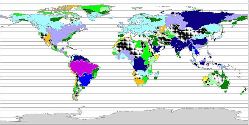
Bundesanstalt für
 Gewässerkunde

Mitteilung Nr. 36

                    List of Figures

                      1    Assignment of WaterGAP 2.2d watersheds to continents . . . . . . . .       .   .   .   .   10
                      2    Assignment of WaterGAP 2.2d watersheds to oceans . . . . . . . . . .       .   .   .   .   10
                      3    Assignment of WaterGAP 2.2d watersheds to GIWA regions . . . . . .         .   .   .   .   11
                      4    Freshwater flux into the World Ocean 1901–2016 (excluding Greenland)       .   .   .   .   14

                      5    Web application: map display . . . . . . . . . . . . . . . . . . . . . . . . . . .         18
                      6    Web application: time series display . . . . . . . . . . . . . . . . . . . . . . .         18
                      7    Web application: tabular display (all numbers are rounded to integer values) . .           19
                      A1   Freshwater fluxes into the World’s oceans of 5° continental coastline cells,
                           GRDC 2004 . . . . . . . . . . . . . . . . . . . . . . . . . . . . . . . . . . . .          24
                      A2   Freshwater fluxes into the World’s oceans of 5° continental coastline cells,
                           GRDC 2004 . . . . . . . . . . . . . . . . . . . . . . . . . . . . . . . . . . . .          27
                      A3   Freshwater fluxes into the World’s oceans from GIWA regions, web map service,
                           GRDC 2014 . . . . . . . . . . . . . . . . . . . . . . . . . . . . . . . . . . . .          29

        page 4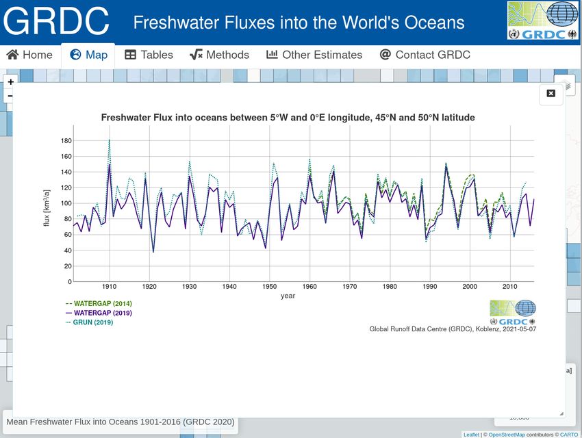
Bundesanstalt für
                                                                                                  Gewässerkunde

                                                                                                  Mitteilung Nr. 36

List of Tables

  1    Mean freshwater fluxes 1901–2016 from continents into World’s oceans . . . .         13
  2    Estimations of freshwater fluxes from World’s continents . . . . . . . . . . . .     15
  3    Estimations of freshwater fluxes into World’s oceans . . . . . . . . . . . . . .     16

  A1   Mean longterm freshwater fluxes from continents into World’s oceans, 2004 edition 24
  A2   Mean freshwater fluxes (1961–1990) from continents into World’s oceans, 2009
       edition . . . . . . . . . . . . . . . . . . . . . . . . . . . . . . . . . . . . . . . 26
  A3   Mean freshwater fluxes (1961–1990) from continents into World’s oceans, 2014
       edition . . . . . . . . . . . . . . . . . . . . . . . . . . . . . . . . . . . . . . . 28

                                                                                                  page 5
Bundesanstalt für
 Gewässerkunde

Mitteilung Nr. 36

                    Zusammenfassung

                    Die Süßwasserzuflüsse in die Weltmeere (Freshwater Fluxes into the World’s Oceans) ist ein
                    Datenprodukt, welches vom Weltdatenzentrum Abfluss (Global Runoff Data Centre, GRDC)
                    erstellt wird. Die aktuellste Berechnung erfolgte im Dezember 2020 und umfasst die Zeitpe-
                    riode 1901–2016. Für die Bereitstellung wurde eine neue Web-Applikation geschaffen, in die
                    auch die 2004, 2009 und 2014 berechneten Daten zu Archivzwecken integriert sind.

                    Grundlage der Berechnungen sind die Ergebnisse der Reanalyse des Wasserhaushaltes mit
                    dem globalen Wasserhaushaltsmodell WaterGAP 2.2d, welche von der AG Hydrologie der
                    Universität Frankfurt 2020 veröffentlicht wurden. Für die Auswertung wurden die auf einem
                    0,5°x0,5°-Raster vorliegenden Rohdaten zu jährlichen Durchschnittswerten für Kontinente
                    und Ozeane, 5°- und 10°-Bänder sowie den von Global International Waters Assessment
                    (GIWA) definierten Regionen aggregiert. Die Darstellung erfolgt sowohl in einer Kartenan-
                    wendung als auch in der seit 1975 verwendeten tabellarischen Struktur.

        page 6
Bundesanstalt für
                                                                              Gewässerkunde

                                                                              Mitteilung Nr. 36

Acronyms

BfG Bundesanstalt für Gewässerkunde (German Federal Institute of Hydrology)

CRU Climate Research Unit

GCOS Global Climate Observing System

GIWA Global International Waters Assessment

GRDC Global Runoff Data Centre

GRUN Global Runoff Reconstruction

R Programming language for statistical computing

RC Runoff Coefficient

UNEP United Nations Environmental Programme

WaterGAP Water Global Assessment and Prognosis

WMO World Meteorological Organization

                                                                              page 7
Bundesanstalt für
Gewässerkunde
Mitteilung Nr. 36
1 Introduction
The GRDC Freshwater Fluxes into the World’s Oceans is a web application provided by the
Global Runoff Data Centre (GRDC) to present the Freshwater Fluxes into the World’s Oceans
data product. Continental freshwater input into the oceans is computed by the GRDC at ir-
regular intervals, most recently in December 2020 referencing the time period 1901–2016.
Previous data sets prepared in 2004, 2009 and 2014 are integrated into the service. The 2004,
2009 and 2014 data sets were not re-calculated and freshwater flux estimates are given as cal-
culated at that time. Map layers present the freshwater fluxes by continent, by ocean or for
specific land areas, for example those associated with the UNEP GIWA Regions (UNEP 2006).
Freshwater fluxes per 5° and 10° latitude bands and through 5° coastline cells show how much
freshwater flows from a specific land area into a specific ocean through a particular stretch of
coast. Tabular summaries present the continental fluxes into 5° or 10° latitude bands within
predefined reference periods. The design of tables consistently follows a template according to
Baumgartner and Reichel (1975) to assure comparability with previous calculations and across
variable reference periods. Estimations of continental runoff or freshwater input to oceans
made by other authors are listed for comparison as documented in literature. This service is
published as an interactive web application (https://shiny.bafg.de/fwf) by the German Federal
Institute of Hydrology (BfG). Disclaimer, Terms and Conditions of the BfG apply. Please cite
in your publication the GRDC as the source of the data: Global Freshwater Fluxes into the
World’s Oceans. Online provided by Global Runoff Data Centre. Koblenz: Federal Institute of
Hydrology (BfG). URL, date of retrieval.
page 8Bundesanstalt für
Gewässerkunde
Mitteilung Nr. 36
2 Technical documentation on the recent
computation 2020
2.1 Workflow reproducibility
In recent years, there have been repeated calls for more reproducibility in hydrological compu-
tations and research (e.g. Hutton et al. 2016; Stagge et al. 2019). Production and publication
of GRDC data products is subject to an ongoing review process with the aim of meeting data
quality requirements arising from e.g. WMO Resolutions 25 (Cg-XIII) and 24 (Cg-18), the
GCOS implementation plan (Wuldera et al. 2016), or from WMO Data Management Prin-
ciples (WMO 2019). The programming language R has established itself as a major tool for
answering the requirements of reproducible and seamless workflows (Slater et al. 2019). For
the 2021 edition of the data product Freshwater Fluxes into the World’s Oceans, a correspond-
ing workflow has been created.
2.2 Input data and computational setting
The input data for the December 2020 computation are:
• WaterGAP v2.2d flow direction scheme (Müller Schmied et al. 2020)
• WaterGAP v2.2d standard model output: river discharge (Müller Schmied et al. 2020)
• continent boundaries (vector polygons, based on Esri 2019)
• ocean boundaries (vector polygons, based on International Hydrographic Organization
1953)
• GIWA regions (vector polygons, based on UNEP 2006)
The WaterGAP 2.2d model operates on the 0.5° x 0.5° CRU grid between 90°N and 60°S. For
this computation of the freshwater fluxes the extent of continents and oceans is specified as
follows:
North America includes Northern America, Greenland, Central America and the Caribbean.
Asia is separated from Europe by Ural Mountains, Ural River, Caspian Sea, Caucasus Moun-
tains, Black Sea, Bosporus and Dardanelles. Australia includes Australia, New Zealand,
Melanesia, Micronesia and Polynesia (aka Oceania). Antarctica excludes the main land and all
islands south of 60°S, but includes islands within the Antarctic Convergence north of 60°S.
The Arctic Ocean includes Hudson Bay, Greenland Sea and Norwegian Sea. The Atlantic
Ocean includes Mediterranean Sea and Black Sea.
page 9Bundesanstalt für
Gewässerkunde
Mitteilung Nr. 36
Except for the Caspian Sea, inland sinks have not been considered in this computation. In
compliance with the previous version, for evaluation the outlet cell of the Amazon river has
been assigned to the southern hemisphere, although in the flow direction scheme it is located
at the 0.25°N, 50°W cell (in the real World, the estuary is situated exactly on the equator).
That means, that the flux from Amazon river is in its entirety assigned to the 10° latitude band
between 0°N and 10°S, to the 5° latitude band between 0°N and 5°S, and to the 5° x 5° cell at
0°N-5°S/50°W-55°W.
South America
North America
Europe
Australia
Asia
Antarctica
Africa
Figure 1: Assignment of WaterGAP 2.2d watersheds to continents
Pacific Ocean
Indian Ocean
Caspian Sea
Atlantic Ocean
Arctic Ocean
Figure 2: Assignment of WaterGAP 2.2d watersheds to oceans
page 10West Greenland Shelf
Norwegian Sea Arctic
East Greenland Shelf
East Bering Sea West Bering Sea
Iceland Shelf Baltic Sea Barents Sea
Baffin Bay, Labrador Sea, Canadian Arch.
North Sea
Newfoundland Shelf Sea of Okhotsk
Gulf of Alaska Caspian Sea
Gulf of St. Lawrence Scotian Shelf Celtic−Biscay Shelf
California Current Sea of Japan Oyashio Current
Black Sea
Iberian Coastal
Gulf of Mexico Northeast Shelf Bohai Sea
Yellow Sea Kuroshio Current
Gulf of California Southeast Shelf The Gulf Arabian Sea
Mediterranean Sea East−China Sea
Canary Current Bay of Bengal
Caribbean Islands
undefined Red Sea
Eastern Equatorial Pacific Mekong River
Guinea Current Gulf of Aden South China Sea
Caribbean Sea
Somali Coastal Current Sulu−Celebes Sea
Amazon
Small Island States
Indonesian Seas
Brazilian Northeast Coral Sea Basin
Benguela Current
Agulhas Current North Australian Shelf
Brazil Current
Great Barrier Reef
Patagonian Shelf
Great Australian Bight
Humboldt Current
Tasman Sea
120°W 60°W 0° 60°E 120°E
Figure 3: Assignment of WaterGAP 2.2d watersheds to GIWA regions
page 11
Gewässerkunde
Bundesanstalt für
Mitteilung Nr. 36Bundesanstalt für
Gewässerkunde
Mitteilung Nr. 36
Standard output of WaterGAP 2.2d model are data in monthly resolution. Because yearly
time steps are used in this computation, the input files were pre-processed with the tool cdo
(Schulzweida 2019):
cdo yearmean watergap_22d_WFDEI-GPCC_histsoc_dis_monthly_1901_2016.nc4 \
watergap_22d_WFDEI-GPCC_histsoc_dis_yearly_1901_2016.nc4
2.3 Processing: new R package fwf
All functions needed to process the freshwater fluxes data product are included in the newly
developed R package fwf. Basic steps are described below.
The first instruction creates a directed graph based on the flow direction map. The resulting
object of data type graph (R-package igraph) allows to quickly determine the catchment area
associated with an outlet cell.
graphBundesanstalt für
Gewässerkunde
Mitteilung Nr. 36
In the last step, a time series object is generated (data type hydtsReg, package hydts):
tsBundesanstalt für
Gewässerkunde
Mitteilung Nr. 36
Figure 4: Freshwater flux into the World Ocean 1901–2016 (excluding Greenland)
The values range between a minimum of 34573 km³ (1993) and a maximum of 42947 km³
(1949). The standard deviation is 1476 km³. The application of the Mann-Kendall trend test
does not show any significant monotonic trend over the entire period. However, looking at
subsections, a significant positive trend is found for the period 1901–1950 (p = 4.80 · 10−5 ) and
a significant negative trend for the period 1951–2000 (p = 1.36 · 10−5 ).
2.5 Comparison with other Estimates
Estimates of freshwater input to the World’s oceans that have been calculated by other authors
are given in table 2 and table 3 as documented in literature. The spatial and temporal settings
are given as described in the source. For further analysis of the methods applied, reference is
made to the source publication.
page 14Table 2: Estimations of freshwater fluxes from World’s continents
Source Reference Period Asia1 Africa North America2 South America Europe3 Australia4 Antarctica Land
Baumgartner and Reichel (1975)*, table 12 not specified 12200 3400 5900 11100 2800 2400 2000 39700
Korzoun et al. (1977)*, table 11 & 12 not specified 14100 4600 8180 12200 2970 2510 2310 47000
Lvovich (1979)*, table 3 not specified 13190 4225 5960a 10380 3110 1965 2200 41730b
Shiklomanov (1993/1999/2000)*, table 2 not specified 13510 4050 7890 12030 2900 2404 not specified 42780
GRDC (1996), table 3 not specified 12559 8585 4309 13578 2446 1231 not specified 42709c
GRDC (2004), online not specified 13848 3690 6294 11896 3083 1722 not specified 40553c
GRDC (2009), online not specified 11603 3511 5475 11083 2752 1685 not specified 36109c
GRDC (2014), online 1961–1990 13754 4250 6856 11796 3367 1844 not specified 41867c
GRDC (2020), this study 1901–2016 12377 4197 6730 11300 2921 2652 8d 40185
Fekete et al. (1999), table 4 not specified 13414e 4474e 6478e 11708e 2673e 712e not specified 39476e
Fekete et al. (2002), table 3, text not specified 13091e 4517e 5982e 11715e 2772e 1320e not specified 39319e
Vörösmarty et al. (2000), table 4 not specified 13700 4520 5890 11700 2770 714 not specified 39300
Oki et al. (2001), table 2 not specified 9385 3616 3824 8789 2191 1680 not specified 29845
Oki et al. (2004), table 2** not specified 10940e 4830e 6210e 11300e 5410e 1940e 1900 42520e
Döll et al. (2003), table 1 1961–1990 11234 3529 5540 11382 2763 2239 not specified 36687c
Syed et al. (2009), table 2, Case: GRACE & ECMWF March 2003–May 2005 7784 2515 6000 9828 1601 185f excluded not specified
Syed et al. (2009), table 2, Case: GRACE & NCEP-NCAR March 2003–May 2005 7938 4717 7104 10332 1299 561f excluded not specified
*
water balance of continents: Pcontinent - Econtinent + Q incl groundwater non-drained by rivers
**
values in the original source are given in 1015 kg/a
a
excl Greenland (700 km3/a)
b
incl Greenland (700 km3/a)
c
excl Antarctica
d
islands within Arctic Convergence, north of 60 latitude
e
including endorheic basins (internal drainage)
f
refers to Australasia
1
separated from Europe by Ural Mountains, Ural River, Caspian Sea, Caucasus Mountains, Black Sea, Bosporus and Dardanelles
2
includes Northern America, Central America and the Caribbean
3
separated from Asia by Ural Mountains, Ural River, Caspian Sea, Caucasus Mountains, Black Sea, Bosporus and Dardanelles
4
includes Australia, New Zealand, Melanesia, Micronesia and Polynesia (aka Oceania)
page 15
Gewässerkunde
Bundesanstalt für
Mitteilung Nr. 36page 16
Mitteilung Nr. 36
Gewässerkunde
Bundesanstalt für
Table 3: Estimations of freshwater fluxes into World’s oceans
3 3
Source Reference Period Arctic1 Atlantic2, 3 Indian Pacific Southern Ocean4 Inland Sinks Sea5
Baumgartner and Reichel (1975)*, table XXXV not specified 2611 19351a 5601a 12137a 528 & 887 & 572b not specified 39700a
Korzoun et al. (1977)*, table 13 & 14 not specified 5200 20800a 6100a 14800a 600 & 800 & 1800b not specified 47000a
Shiklomanov (1993/1999/2000)*, table 11 not specified 4281 19799 4858 12211 not specified not specified 41115
GRDC (2004), online not specified 3864 20373 5051 11245 not specified 800c 40971
GRDC (2009), online not specified 3197 19127 4251 9534 not specified 682c 36109
GRDC (2014), online 1961–1990 4080 20722 5238 11826 not specified 692c 41867
GRDC (2020), this study 1901–2016 4442 18719 5139 11531 not specified 353c 39831
Fekete et al. (1999), table 4 not specified 2947d 18357d & 1169e 4802d 11127d not specified 1075 39476d
Fekete et al. (2002), table 5 not specified 3268d 19711d 4862d 10479d not specified not specified 38320d
Dai and Trenberth (2002), table 4, Case: 921 rivers not specified 3658 19168 & 838e 4532 9092 not specified not specified 37288
Dai and Trenberth (2002), table 4, Case: ECMWF P-E 1979–1993 3967 20585 & 1144e 4989 7741 not specified not specified 38426
Dai and Trenberth (2002), table 4, Case: NCEP-NCAR P-E 1979–1995 4358 16823 & 909e 3162 7388 not specified not specified 32640
Oki et al. (2004), table 2 ** not specified 3660 16300f & 4320g 4320 6780f & 2560g 3660 2020 42520
Syed et al. (2009), table 4, Case: GRACE & ECMWF March 2003–May 2005 3482 14998 1686 7988 not specified not specified not specified
Syed et al. (2009), table 4, Case: GRACE & NCEP-NCAR March 2003–May 2005 3654 18107 1668 9080 not specified not specified not specified
Wisser et al. (2010), Table 2, Case: natural conditions 1901–2002 2288 18340d & 1197e 4983 9853 not specified 1072 37984
Wisser et al. (2010), table 2, Case: disturbed conditions 1901–2002 2282 18305d & 1168e 5525 9626 not specified 1037 37401
Milliman and Farnsworth (2011), table 2.4 not specified 4800 13200f & 3400g 4000 6100f & 4100g not specified not specified 36000
*
water balance of oceans: Pocean - Eocean + Q, Q incl groundwater non-drained by rivers
**
values in the original source are given in 1015 kg/a
a
including Southern Ocean
b
southern parts of Atlantic, Indian and Pacific ocean
c
Lake Aral & Caspian Sea only
d
including endorheic basins
e
Mediterranean and Black Sea
f
northern portion of the ocean
g
southern portion of the ocean
1
including Hudson Bay, Greenland Sea and Norwegian Sea
2
including Mediterranean Sea and Black Sea
3
separated from Southern Ocean along the Antarctic Convergence line
4
separated from Atlantic, Indian and Pacific Oceans along the Antarctic Convergence line
5
excluding inland sinksBundesanstalt für
Gewässerkunde
Mitteilung Nr. 36
3 Web Application
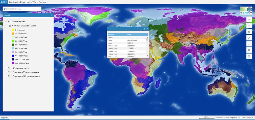
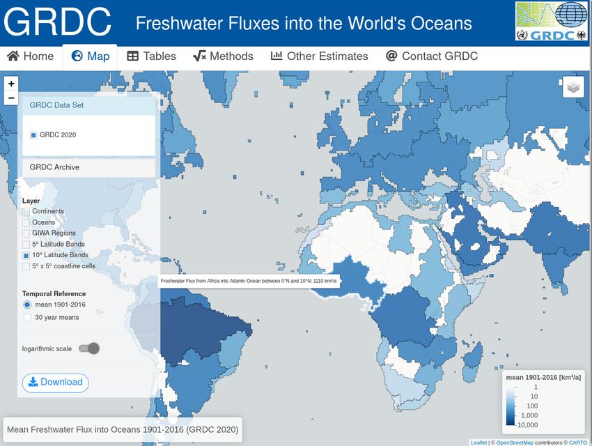
The Freshwater Fluxes into the World’s Oceans 2020 are presented in a new web application,
which also integrated the results of the previous versions as calculated in 2004, 2009 and 2014.
Map layers show the mean freshwater fluxes in km³/a for the period 1901–2016 as well as for
30-year periods including the WMO reference periods 1931–1960 and 1961–1990 (figure 5).
For each selected region a graph (figure 6) shows the fluxes for the entire period, compared
to the results of the edition 2014 and to a global gridded reconstruction of runoff covering the
period 1902–2014 (GRUN).
The GRUN reconstruction used a machine learning algorithm trained by observation data to
derive monthly river discharges based on precipitation and temperature from an atmospheric
reanalysis (Ghiggi et al. 2019). When comparing to the GRUN dataset, it should be noted that
the GRUN model is not coupled to a routing module. Evaporation losses through lakes and
reservoirs as well as water withdrawals are therefore not considered, in contrast to WaterGAP,
which can lead to a large overestimate of the total flux. For large catchments, this also leads to
a negative offset of the discharge amplitudes. Since the GRUN dataset covers a similar time
period as the WaterGAP 2.2d dataset, it is presented for comparison, with reference to the
limitations. Tabular summaries of freshwater fluxes into 5° and 10° latitude bands are given
for the entire reference period, 30-year periods and decadal intervals (figure 7).
page 17Bundesanstalt für
Gewässerkunde
Mitteilung Nr. 36
Figure 5: Web application: map display
Figure 6: Web application: time series display
page 18Figure 7: Web application: tabular display (all numbers are rounded to integer values)
page 19
Gewässerkunde
Bundesanstalt für
Mitteilung Nr. 36Bundesanstalt für
Gewässerkunde
Mitteilung Nr. 36
References
Baumgartner, Albert, and Eberhard Reichel. 1975. The World water balance. Vol. 179. Elsevier
New York.
Couet, T. de, and T. Maurer. 2004. “Surface freshwater fluxes into the World oceans. Online
edition 2004.” Global Runoff Data Centre. Koblenz: Federal Institute of Hydrology (BfG).
———. 2009. “Surface Freshwater Fluxes into the World Oceans. Online edition 2009.” Global
Runoff Data Centre. Koblenz: Federal Institute of Hydrology (BfG).
Dai, Aiguo, and Kevin E Trenberth. 2002. “Estimates of freshwater discharge from continents:
Latitudinal and seasonal variations.” Journal of Hydrometeorology 3 (6): 660–87.
Döll, Petra, Frank Kaspar, and Bernhard Lehner. 2003. “A global hydrological model for
deriving water availability indicators: model tuning and validation.” Journal of Hydrology 270
(1-2). Elsevier: 105–34.
Esri. 2019. “World Continents.”
Fekete, Balazs M, Charles J Vörösmarty, and Wolfgang Grabs. 1999. “Global, composite runoff
fields based on observed river discharge and simulated water balances.” Global Runoff Data
Centre Koblenz.
Ghiggi, Gionata, Vincent Humphrey, Sonia I Seneviratne, and Lukas Gudmundsson. 2019.
“GRUN: an observation-based global gridded runoff dataset from 1902 to 2014.” Earth System
Science Data 11 (4). Copernicus GmbH: 1655–74.
Grabs, W., T. de Couet, and J. Pauler. 1996. “Freshwater fluxes from continents into the World
Oceans based on data of the Global Runoff Data Base.” Federal Institute of Hydrology (BfG).
Hutton, Christopher, Thorsten Wagener, Jim Freer, Dawei Han, Chris Duffy, and Berit Arheimer.
2016. “Most computational hydrology is not reproducible, so is it really science?” Water
Resources Research 52 (10). Wiley Online Library: 7548–55.
International Hydrographic Organization. 1953. “Limits of Oceans and Seas—Special Publica-
tion 23.” IHO Monte Carlo, Monaco.
Lvovitch, M. I. 1973. “The global water balance.” Eos, Transactions American Geophysical
Union 54 (1): 28–53. doi:https://doi.org/10.1029/EO054i001p00028.
Milliman, John D, and Katherine L Farnsworth. 2013. River discharge to the coastal ocean: a
global synthesis. Cambridge University Press.
page 20Bundesanstalt für
Gewässerkunde
Mitteilung Nr. 36
Müller Schmied, Hannes, Denise Cáceres, Stephanie Eisner, Martina Flörke, Claudia
Herbert, Christoph Niemann, Thedini Asali Peiris, et al. 2020. “The global water re-
sources and use model WaterGAP v2.2d - Standard model output.” Data set. PANGAEA.
doi:10.1594/PANGAEA.918447.
Oki, Taikan, Yasushi Agata, Shinjiro Kanae, Takao Saruhashi, Dawen Yang, and Katumi Musiake.
2001. “Global assessment of current water resources using total runoff integrating pathways.”
Hydrological Sciences Journal 46 (6). Taylor & Francis: 983–95.
Oki, Taikan, Dara Entekhabi, and Timothy Ives Harrold. 1999. “The global water cycle.” Global
Energy and Water Cycles 10. Cambridge University Press Cambridge: 27.
Schulzweida, Uwe. 2019. “CDO User Guide.” doi:10.5281/zenodo.3539275.
Shiklomanov, I. A. 2009. “World water resources and their use.” joint SHI/UNESCO product.
https://hydrologie.org/DON/html.
Slater, Louise J, Guillaume Thirel, Shaun Harrigan, Olivier Delaigue, Alexander Hurley, Abdou
Khouakhi, Ilaria Prosdocimi, Claudia Vitolo, and Katie Smith. 2019. “Using R in hydrology: a
review of recent developments and future directions.” Hydrology and Earth System Sciences 23
(7). EGU: 2939–63.
Stagge, James H, David E Rosenberg, Adel M Abdallah, Hadia Akbar, Nour A Attallah, and
Ryan James. 2019. “Assessing data availability and research reproducibility in hydrology and
water resources.” Scientific Data 6 (1). Nature Publishing Group: 1–12.
Syed, Tajdarul H, James S Famiglietti, and Don P Chambers. 2009. “GRACE-based estimates of
terrestrial freshwater discharge from basin to continental scales.” Journal of Hydrometeorology
10 (1): 22–40.
UNEP. 2006. “Challenges to international waters: Regional assessments in a global perspective.”
United Nations Environment Programme, Nairobi, Kenya.
USSR National Committee for the International Hydrological decade and Korzun, Valentin
Ignatevich. 1977. Atlas of World water balance. Unesco Press.
Vörösmarty, Charles J, Pamela Green, Joseph Salisbury, and Richard B Lammers. 2000. “Global
water resources: vulnerability from climate change and population growth.” Science 289 (5477).
American Association for the Advancement of Science: 284–88.
Wilkinson, K., M. von Zabern, and J. Scherzer. 2014. “Global freshwater fluxes into the World
oceans. Online edition 2014.” Global Runoff Data Centre. Koblenz: Federal Institute of
Hydrology (BfG).
Wisser, Dominik, Balazs M Fekete, CJ Vörösmarty, and AH Schumann. 2010. “Reconstructing
20th century global hydrography: a contribution to the Global Terrestrial Network-Hydrology
(GTN-H).” Hydrology and Earth System Sciences 14 (1). Copernicus: 1–24.
WMO. 2019. Manual on the High-quality Global Data Management Framework for Climate.
Geneva, Switzerland: World Meteorological Organization.
page 21Bundesanstalt für
Gewässerkunde
Mitteilung Nr. 36
Wuldera, MA, JC White, TR Loveland, CE Woodcock, A Belward, and WB Cohen. 2016. “The
global observing system for climate: implementation needs. GCOS Implementation Plan 2016,
GCOS-200 (GOOS-214).”
page 22Bundesanstalt für
Gewässerkunde
Mitteilung Nr. 36
Annex 1: Freshwater Fluxes into the World’s
Oceans (GRDC, 2004)
The 2004 edition was only published online on the GRDC website. This editorial summary is
based on excerpts from the online publication at the GRDC website 2004. The result tables
of freshwater fluxes into 5° or 10° latitude bands are integrated in the Freshwater Fluxes to
the World Oceans web service (fwf.grdc.bafg.de). The freshwater flux estimates are given as
published in 2004.
Freshwater input from continents into the oceans is of major interest in research concerned
with global monitoring of freshwater resources, the flux of matter into coastal areas and the
sea, or the influence of freshwater fluxes on circulation patterns on regional and global scales.
For clarification: The term freshwater flux is used here for continental surface runoff that
flows into the oceans through rivers.
In 1995, a first estimation of continental runoff as well as freshwater fluxes into the oceans
was published by GRDC based on river discharge data collected in the Global Runoff
Database (Grabs, Couet, and Pauler 1996). At that time, the continental runoff through
rivers was extrapolated from catchment-related fluxes calculated as the sum of annual runoff
volumes from catchment areas that are represented by one of 194 selected GRDC stations
close to the river mouth. Rivers draining into the Caspian, the Mediterranean and the Baltic
Sea were excluded.
In 2004, the mean annual Surface Freshwater Fluxes into the World Oceans has been re-
calculated on the basis of new observation data and using a 0.5° flow direction grid. The area
extrapolation has been replaced by runoff coefficients (RC) in order to better capture the land
areas that are not covered by observation data. For grid cells that form the edge of the conti-
nents the integral freshwater flux from hinterland catchments was calculated as the spatially
weighted product of a runoff coefficient and the precipitation. Excluding internal runoff, a
long-term total volume of 40.533 km³/a from continents (except Antarctica and islands) into
the four oceans (see table A1) was estimated.
For 251 watersheds whose outlet is represented by a GRDC station close to the mouth and
representing an upstream catchment greater than 25,000 km², the long-term annual runoff was
derived from observed river discharge. A runoff coefficient (RC) for the upstream catchment
was calculated by relating the observed discharge at this station to the catchment area and the
mean monthly precipitation in the period 1961-1990. RC was used to estimate a mean annual
runoff from land areas not integrally captured by a GRDC station by means of regionalization
page 23Bundesanstalt für
Gewässerkunde
Mitteilung Nr. 36
Table A1: Mean longterm freshwater fluxes from continents into World’s oceans, 2004 edition
Arctic Ocean Atlantic Ocean Indian Ocean Pacific Ocean Sum Sea*
Europe 666 2417 - - 3083
Asia 2349 6 4174 7320 13848
Africa - 2906 784 - 3690
Australia - - 95 1627 1722
North America 849 3761 - 1685 6294
South America - 11283 - 614 11897
Sum Land* 3863 20373 5051 11245 40533
* slight deviations due to rounding
from nearby monitored areas considering the observed discharge of additional 1378 GRDC
stations close to the coast of continents.
Using a 0.5° elevation grid optimized for flow path detection (Döll and Lehner 2002) the
hinterland catchments upstream of approx. 12.000 individual grid cells that form the edge of
the continents were determined, and the continental grid cells co-registered with a edge grid
cell through which they drain into an ocean or internal sink. Each edge grid cell got assigned
either a calculated or estimated RC to calculate the integral flux from its adjacent catchment as
the spatially weighted product of RC and precipitation over all co-registered grid cells.
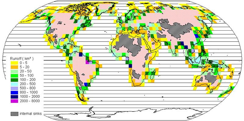
Figure A1: Freshwater fluxes into the World’s oceans of 5° continental coastline cells, GRDC
2004
Freshwater fluxes through specific coastline sections were calculated by summarizing the
fluxes for subsets of continental edge cells. For example, freshwater input was calculated
for the sub-regions defined by the Global International Waters Assessment initiative GIWA
(UNEP 2006) as well as for a 5° and 10° grid. Figure A1 shows the freshwater fluxes through
the 5° grid cells along the coasts of the continents. The freshwater fluxes into 5° or 10° lati-
page 24Bundesanstalt für
Gewässerkunde
Mitteilung Nr. 36
tude bands given in a table using a template according to Baumgartner and Reichel (1975),
became part of the Freshwater Fluxes to the World Oceans web service (fwf.grdc.bafg.de).
References of edition 2004:
Baumgartner, Albert, and Eberhard Reichel. 1975. The World water balance. Vol. 179. Elsevier
New York.
Döll, Petra, and Bernhard Lehner. 2002. “Validation of a new global 30-min drainage direction
map.” Journal of Hydrology 258 (1-4). Elsevier: 214–31.
Grabs, W., T. de Couet, and J. Pauler. 1996. “Freshwater fluxes from continents into the World
Oceans based on data of the Global Runoff Data Base.” Federal Institute of Hydrology (BfG).
UNEP. 2006. “Challenges to international waters: Regional assessments in a global perspective.”
United Nations Environment Programme, Nairobi, Kenya.
page 25Bundesanstalt für
Gewässerkunde
Mitteilung Nr. 36
Annex 2: Freshwater Fluxes into the World’s
Oceans (GRDC, 2009)
The 2009 edition was only published online on the GRDC website. This editorial summary is
based on excerpts from the online publication at the GRDC website 2009. The result tables
of freshwater fluxes into 5° or 10° latitude bands are integrated in the Freshwater Fluxes to
the World Oceans web service (fwf.grdc.bafg.de). The freshwater flux estimates are given as
published in 2009.
Freshwater input from continents into the oceans is of major interest in research concerned
with global monitoring of freshwater resources, the flux of matter into coastal areas and the
sea, or the influence of freshwater fluxes on circulation patterns on regional and global scales.
For clarification: The term freshwater flux is used here for continental surface runoff that
flows into the oceans through rivers.
In 2009, the mean annual Surface Freshwater Fluxes into the World Oceans has been re-
calculated on basis of runoff volumes simulated with the Global Hydrology Model WaterGAP
2.1 at a spatial resolution of 0.5°. Referencing the period from 1961 to 1990, a long-term total
volume of 36.109 km³/a from continents into the four oceans (see table A2) was estimated.
Table A2: Mean freshwater fluxes (1961–1990) from continents into World’s oceans, 2009
edition
Arctic Ocean Atlantic Ocean Indian Ocean Pacific Ocean Sum Sea*
Europe 451 2301 - - 2752
Asia 2108 10 3309 6177 11603
Africa - 2742 768 - 3511
Australia - - 174 1511 1685
North America 638 3515 - 1322 5475
South America - 10560 - 524 11083
Sum Land* 3197 19127 4251 9534 36109
* slight deviations due to rounding
In contrast to previous versions, the 2009 edition is completely based on simulated annual
runoff volumes at a 0.5° grid (55 km by 55 km at the Equator), computed by a team at the
University of Frankfurt using the Global Hydrology Model WaterGAP 2.1 (not considering
Antarctica and Greenland). A daily water balance was calculated for 66.896 grid cells, consid-
ering canopy, snow and soil water, groundwater or surface water storages, and as well impacts
page 26Bundesanstalt für
Gewässerkunde
Mitteilung Nr. 36
from human water consumption. River discharge of one grid cell integrated local inflow and
inflow from upstream cells. The WaterGAP model was individually tuned for each sub-basin
based on observed river discharges (Hunger and Döll 2008).
The discharge value computed for one 0.5° catchment cell was routed downstream from cell
to cell to the coastline cell that forms the outlet of the catchment, using the global drainage
direction map DDM30 (P. Döll and Lehner 2002).
Figure A2: Freshwater fluxes into the World’s oceans of 5° continental coastline cells, GRDC
2004
By combining the runoff volumes of the 0.5° coastline cells, freshwater fluxes from specific
hinterland catchments into specific oceans were calculated, for example the freshwater input
from sub-regions defined by the Global International Waters Assessment initiative GIWA
(UNEP 2006), as shown in figure A2. The freshwater fluxes into 5° or 10° latitude bands given
in a table using a template according to Baumgartner and Reichel (1975), became part of the
Freshwater Fluxes to the World Oceans web service (https://shiny.bafg.de/fwf).
References of edition 2009:
Baumgartner, Albert, and Eberhard Reichel. 1975. The World water balance. Vol. 179. Elsevier
New York.
Döll, Petra, and Bernhard Lehner. 2002. “Validation of a new global 30-min drainage direction
map.” Journal of Hydrology 258 (1-4). Elsevier: 214–31.
Hunger, M, and P Döll. 2008. “Value of river discharge data for global-scale hydrological
modeling.” Hydrology and Earth System Sciences 12 (3). Copernicus GmbH: 841–61.
UNEP. 2006. “Challenges to international waters: Regional assessments in a global perspective.”
United Nations Environment Programme, Nairobi, Kenya.
page 27Bundesanstalt für
Gewässerkunde
Mitteilung Nr. 36
Annex 3: Freshwater Fluxes into the World’s
Oceans (GRDC, 2014)
The 2014 edition was published as a stand-alone web service on the GRDC website. This
editorial summary is based on excerpts from the online publication at the GRDC website 2014.
The annual freshwater fluxes computed in 2014 were integrated in the Freshwater Fluxes to
the World Oceans web service (fwf.grdc.bafg.de). The freshwater flux estimates are given as
published in 2014.
Freshwater input from continents into the oceans is of major interest in research concerned
with global monitoring of freshwater resources, the flux of matter into coastal areas and the
sea, or the influence of freshwater fluxes on circulation patterns on regional and global scales.
For clarification: The term freshwater flux is used here for continental surface runoff that
flows into the oceans through rivers.
In 2014, the Global Freshwater Fluxes into the World Oceans has been updated on the basis
of new model results from an improved Global Hydrology Model WaterGAP 2.2 at a spatial
resolution of 0.5°. Referencing the period from 1961 to 2009, a long-term total volume of
41.867 km³/a from continents into the four oceans (see table A3) was estimated.
Table A3: Mean freshwater fluxes (1961–1990) from continents into World’s oceans, 2014
edition
Arctic Ocean Atlantic Ocean Indian Ocean Pacific Ocean Sum Sea*
Europe 655 2712 - - 3367
Asia 2498 15 3996 7245 13754
Africa - 3130 1120 - 4250
Australia - - 121 1723 1844
North America 927 4028 - 1901 6856
South America - 10838 - 958 11796
Sum Land* 4080 20722 5238 11826 41867
* slight deviations due to rounding
As in the 2009 re-calculation, the estimates of freshwater fluxes are based on simulated annual
runoff volumes at a 0.5° grid, computed by a team at the University of Frankfurt using the
updated Global Hydrology Model WaterGAP 2.2 (not considering Antarctica and Greenland).
Daily river discharges and storages at a spatial resolution of 0.5° were simulated for the whole
land area (66.896 cells). The model was calibrated against observed river discharge at 1319
page 28Bundesanstalt für
Gewässerkunde
Mitteilung Nr. 36
gauging stations around the World, and the adjusted calibration factor regionalized to grid
cells outside of the calibration basins. Since the initial publication of the WaterGAP model
(Döll, Kaspar, and Lehner 2003), major changes were made to keep the model up to date
(Müller Schmied et al. 2014).
The discharge value computed for one 0.5° catchment cell was transferred downstream along a
river network using the global drainage direction map DDM30 (Döll and Lehner 2002) to the
0.5° coastline cell that forms the outlet of the catchment.
Figure A3: Freshwater fluxes into the World’s oceans from GIWA regions, web map service,
GRDC 2014
The 2014 edition was published as a stand-alone Web Map Service providing annual means
of continental freshwater input from GIWA regions, through 5° coastline cells and into 5° and
10° latitude bands. The results published online in the web map service became part of the
Freshwater Fluxes to the World Oceans web service (fwf.grdc.bafg.de), as well as the tabular
summaries of freshwater fluxes into 5° or 10° latitude bands using a template according to
Baumgartner and Reichel (1975),
References of edition 2014:
Baumgartner, Albert, and Eberhard Reichel. 1975. The World water balance. Vol. 179. Elsevier
New York.
Döll, Petra, and Bernhard Lehner. 2002. “Validation of a new global 30-min drainage direction
map.” Journal of Hydrology 258 (1-4). Elsevier: 214–31.
Döll, Petra, Frank Kaspar, and Bernhard Lehner. 2003. “A global hydrological model for
deriving water availability indicators: model tuning and validation.” Journal of Hydrology 270
(1-2). Elsevier: 105–34.
Müller Schmied, Hannes, Stephanie Eisner, Daniela Franz, Martin Wattenbach, Felix Theodor
Portmann, Martina Flörke, and Petra Döll. 2014. “Sensitivity of simulated global-scale fresh-
water fluxes and storages to input data, hydrological model structure, human water use and
page 29Bundesanstalt für
Gewässerkunde
Mitteilung Nr. 36
calibration.” Hydrology and Earth System Sciences 18 (9). Copernicus GmbH: 3511–38.
page 30In der Reihe BfG-Mitteilungen sind bisher u. a. erschienen:
Nr. 13 Molekularbiologische Grundlagen und limnologische Bedeutung der Lichthemmung (Photoinhibition)
der Photosynthese in Fließgewässern – Literaturstudie. Koblenz 1997, 48 S.
Nr. 14 Festschrift zum 50jährigen Jubiläum. Koblenz, Januar 1998, 72 S.
Nr. 15 Schadstoffbelastung der Sedimente in den Ostseeküstengewässern. Koblenz, Juli 1998, 124 S.
Nr. 16 Zukunft der Hydrologie in Deutschland. Tagung vom 19.-21. Januar 1998 in Koblenz. Koblenz, Oktober
1998, 224 S.
Nr. 17 Der Main – Fluß und Wasserstraße. Vortragsveranstaltung des Wasserstraßenneubauamtes Aschaffenburg
am 5. und 6. Mai 1997 in Würzburg. Koblenz, November 1998, 148 S.
Nr. 18 Erfolgskontrollen an Bundeswasserstraßen – Beweissicherung für Eingriffsbeurteilung und Kompensa-
tionsmaßnahmen. Beiträge zum Kolloquium am 18.11.1997 in Koblenz. Koblenz, Februar 1999, 52 S.
Nr. 19 Mathematische Modelle in der Gewässerkunde – Stand und Perspektiven. Beiträge zum Kolloquium am
15./16.11.1998 in Koblenz. Koblenz, August 1999, 130 S.
Nr. 20 Umweltverträglichkeitsuntersuchungen an Bundeswasserstraßen – Materialien zur Behandlung von
Alternativen und Wechselwirkungen sowie zur Durchführung der Verträglichkeitsprüfung nach FFH-
Richtlinie. Koblenz, Februar 2000, 64 S.
Nr. 21 GIS-gestützte hydrologische Kartenwerke in Mitteleuropa. Beiträge zum internationalen Workshop vom
12.-14.10.1999 in Koblenz. Koblenz, Juli 2000, 199 S.
Nr. 22 Sedimentbewertung in europäischen Flussgebieten – Sediment Assessment in European River Basins.
Beiträge zum internationalen Symposium vom 12.-14. April 1999 in Berlin. Koblenz, November 2000,
196 S. (deutsch/englisch)
Nr. 23 Bewertung von großen Fließgewässern mittels Potamon-Typie-Index (PTI). Verfahrensbeschreibung und
Anwendungsbeispiele. Koblenz, Februar 2001, 28 S.
Nr. 24 Mathematisch-numerische Modelle in der Wasserwirtschaft. Handlungsempfehlung für Forschungs- und
Entwicklungsarbeiten. Koblenz, Mai 2002, 56 S.
Nr. 25 Einsatz von ökologischen Modellen in der Wasser- und Schifffahrtsverwaltung. Das integrierte Flussauen-
modell INFORM, Koblenz, Mai 2003, 212 S.
Nr. 26 Methode der Umweltrisikoeinschätzung und FFH-Verträglichkeitseinschätzung für Projekte an Bun-
deswasserstraßen. – Ein Beitrag zur Bundesverkehrswegeplanung – , Koblenz, Mai 2004, 23 S. + Anla-
gen
Nr. 27 Niedrigwasserperiode 2003 in Deutschland. Ursachen – Wirkungen – Folgen. Koblenz, Oktober 2006,
212 S. + CD
Nr. 28 Möglichkeiten zur Verbesserung des ökologischen Zustands von Bundeswasserstraßen. Fallbeispielsamm-
lung. Koblenz, März 2009, 36 S.
Nr. 29 Das hydrologische Extremjahr 2011: Dokumentation, Einordnung, Ursachen und Zusammenhänge.
Koblenz, Januar 2014, 164 S. + CD
Nr. 30 Fachbeiträge zum Sedimentmanagementkonzept Elbe. Koblenz, Dezember 2014, 164 S.
Nr. 31 Das Hochwasserextrem des Jahres 2013 in Deutschland: Dokumentation und Analyse. Koblenz, Dezem-
ber 2014, 232 S.
Nr. 32 Vergleich neuartiger Geräte zur Schwebstoffgewinnung für das chemische Gewässermonitoring
SCHWEBSAM. Koblenz, März 2015, 80 S.
Nr. 33 WSV-Lab – ein Managementwerkzeug zur qualitativ-gewässerkundlichen Bearbeitung von Baggermaß-
nahmen der WSV. Koblenz, September 2015, 40 S.
Nr. 34 Historische Abflussdaten für die Elbe – Ableitung von Tagesabflüssen am Pegel Magdeburg-Strombrücke
im Zeitraum von 1727 bis 1890. Koblenz, Februar 2020, 68 S.You can also read


