Hough Transforms and 3D SURF for robust three dimensional classification
←
→
Page content transcription
If your browser does not render page correctly, please read the page content below
Hough Transforms and 3D SURF for robust
         three dimensional classification

      Jan Knopp1 , Mukta Prasad2 , Geert Willems1 , Radu Timofte1 , and
                             Luc Van Gool1,2
                                 1
                                     KU Leuven, 2 ETH Zurich

       Abstract. Most methods for the recognition of shape classes from 3D
       datasets focus on classifying clean, often manually generated models.
       However, 3D shapes obtained through acquisition techniques such as
       Structure-from-Motion or LIDAR scanning are noisy, clutter and holes.
       In that case global shape features—still dominating the 3D shape class
       recognition literature—are less appropriate. Inspired by 2D methods,
       recently researchers have started to work with local features. In keep-
       ing with this strand, we propose a new robust 3D shape classification
       method. It contains two main contributions. First, we extend a robust
       2D feature descriptor, SURF, to be used in the context of 3D shapes.
       Second, we show how 3D shape class recognition can be improved by
       probabilistic Hough transform based methods, already popular in 2D.
       Through our experiments on partial shape retrieval, we show the power
       of the proposed 3D features. Their combination with the Hough trans-
       form yields superior results for class recognition on standard datasets.
       The potential for the applicability of such a method in classifying 3D
       obtained from Structure-from-Motion methods is promising, as we show
       in some initial experiments.

1    Introduction
A number of methods for 3D shape class recognition have been proposed already.
So far, the dominant line of work has been to use global features, i.e. features
that need the complete, isolated shape for their extraction. Examples are Fourier
or spherical harmonics [1, 2], shape moments [2], shape histograms [3]. There are

                      SfM

                                                                                CLASS
                                              shape                class
                  scanning                                                        OF
                                            description         recognition
                                                                              THE SHAPE
               modelling

          3D shape acquisition

Fig. 1. Proposed approach classifies noisy 3D shapes obtained from SfM, scans etc.
The method is invariant to the texture and recognizes difficult objects such as plants.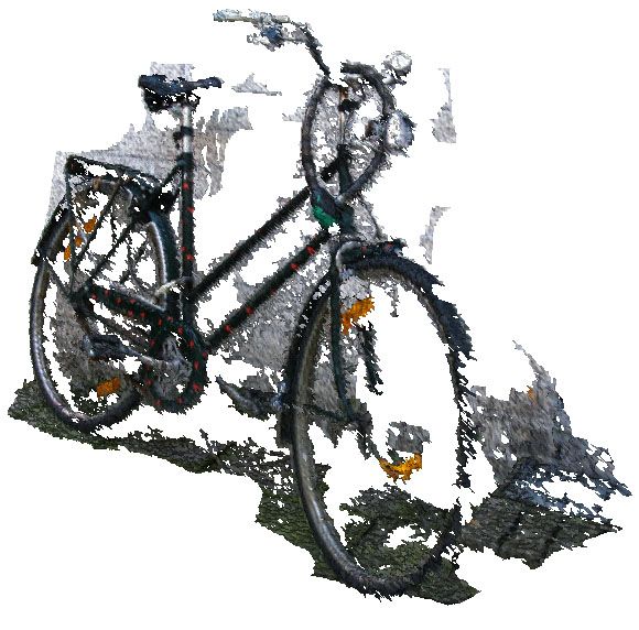
2      J. Knopp, M. Prasad, G. Willems, R. Timofte, L. Van Gool

at least three potential problems with these global approaches: (i) it is diffi-
cult to handle partial shapes. For instance, when an artifact has been damaged,
even the most perfect scan will still only capture a part of what the original
shape should have been, (ii) many capturing scenarios contain irrelevant, neigh-
bouring clutter in addition to the relevant data coming from the object. Global
methods mix the two, jeopardizing class recognition. Some local, skeleton-based
descriptions are also known to suffer from these problems (e.g. [4]), (iii) several
classes contain deformable shapes, some parts of which may be more deformable
than other more rigid parts. Global methods are also less successful at handling
intra-class variations while remaining sufficiently discriminative to noise, clut-
ter, articulated deformations and inter-class variations. In many 3D application
based on retrieval, classification and detection, all these three problems have to
be addressed.
    As work in 2D object class recognition has shown, the use of local rather
than global features is advantageous. 2D class detection methods deal with oc-
clusions and clutter quite successfully already. We therefore seek to apply these
techniques to the 3D case as well. So far, relatively few 3D categorisation meth-
ods based on local features, like tensors [5], heat kernel signatures [6], integral
shape descriptors [7, 8], and scale dependent features [9] have been proposed.
    Ovsjanikov et al. [10] extended the standard bag-of-features (BOF) approach
of Sivic and Zisserman [19] by looking for the frequency of word pairs instead
of the single word, called spatially-sensitive bags of features. Toldo et al. [11]
described 3D shapes by splitting them into segments, which are then described
on the basis of their curvature characteristics. These descriptors are quantized
into a visual vocabulary. Finally, an SVM is learnt for the actual categorisation.
Methods that use other information than pure shape (e.g. [12, 13]) are not con-
sidered here because we are interested in the still-common case where no other
information is available.
    The afore-mentioned methods assume clean, pre-segmented shapes, i.e. with-
out them being attached to a 3D ‘background’. As such, these BOF approaches
could suffer from the problem that the information can get buried under clut-
ter, especially when the object of interest is small compared to this background.
In 3D this difference is magnified. For instance, a statue of a person in front
of a building may cover a large part of the 2D image scene, but will be tiny
compared to the size of the building in 3D, where all objects appear with their
actual, relative scales. In Hough transform based approaches, the process of
recognition is tied up with hypothesis verification (through object localization).
This means that it has higher discriminative power against clutter than BOF
based approaches.
    This paper proposes an approach to 3D shape categorisation that can perform
better at the tasks described above. A 3D extension to SURF [14] serves as
our local descriptor described in § 2. This feature has proved quite effective
in 2D and can now be viably computed even in 3D. In contrast to a dense or
random coverage with spin images [15], a 3D interest point detector picks out a
repeatable and salient set of interest points. These descriptors are quantized and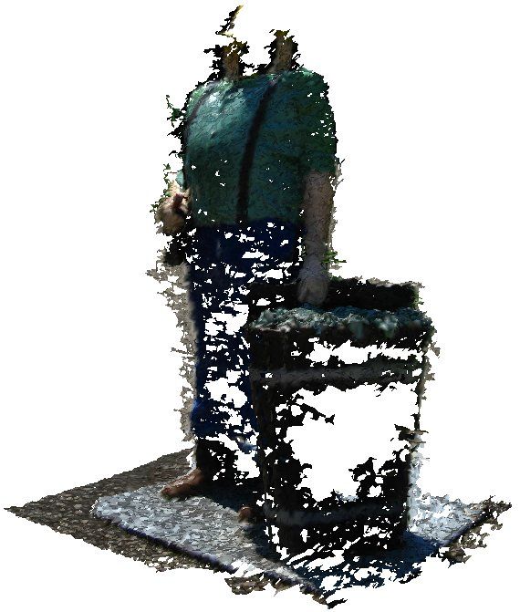
Hough Transforms and 3D SURF for robust three dimensional classification 3
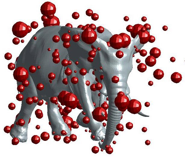
(a) (b) (c)
Fig. 2. Illustration of the detection of 3D SURF features. The shape (a) is voxelized
into the cube grid (side of length 256) (b). 3D SURF features are detected and back-
projected to the shape (c), where detected features are represented as spheres and with
the radius illustrating the feature scale.
used in a Hough approach, like Implicit Shape Model (ISM) [16], which keeps
the influence of each feature better localized than in a BOF approach as seen
in § 3. Our approach favorably compares to the state-of-the-art in 3D shape class
recognition and retrieval as seen in § 4, § 5.
2 Shape representation as the set of 3D SURF features
For our problem of class recognition, we collected a set M of shapes separated
into two disjoint sets: (i) training data MT and (ii) query data MQ . The mth
3D shape is represented as {Vm , Fm }, where Vm is a collection of vertices and Fm is
a collection of polygons (specifically triangles) defined on these vertices.
In order to describe each shape m ∈ M as a set of local rotation and scale-
invariant interest points, we propose an extension of SURF to 3 dimensions.
It is important to note at this point, that this extension can also be seen as
a special case of the recently proposed Hessian-based spatio-temporal features
by Willems et al. [17], where temporal and spatial scale are identical. As such,
the theoretical results that were obtained from scale space theory still hold.
Furthermore, most of the implementation details can be reused, except the fact
that the search space has now shrunk from 5 to 4 dimensions (x, y, z, σ). For
more in-depth information on Hessian-based localization and scale selection in
3 dimensions, we refer the reader to [17].
The extraction of the 3D features is as follows. First, we voxelize a shape in a
volumetric 3D cube of size 2563 using the intersection of faces with the grid-bins
as shown in figure 2(b), after each shape is uniformly scaled to fit the cube while
accounting for a boundary of 40 at each side. The cube parameters were chosen
empirically. Next, we compute a saliency measure S for each grid-bin x and
several scales σ (over three octaves). We define S as the absolute value of the
determinant of the Hessian matrix H(x, σ) of Gaussian second-order derivatives
L(x, σ) computed by box filters,
4 J. Knopp, M. Prasad, G. Willems, R. Timofte, L. Van Gool
Lxx (x, σ) Lxy (x, σ) Lxz (x, σ)
S(x, σ) = H(x, σ) = Lyx (x, σ) Lyy (x, σ) Lyz (x, σ) , (1)
Lzx (x, σ) Lzy (x, σ) Lzz (x, σ)
as proposed in [17]. This has as implication that, unlike in the case of SURF [14],
a positive value of S does not guarantee that all eigenvalues of H have identi-
cal signs. Consequently, not only blob-like signals are detected, but also saddle
points. Finally, Km unique features: dmk , k ∈ {1 . . . Km } are extracted from the
volume using non-maximal suppression (see [17] for more details).
In a second stage, a rotation and scale-invariant 3D SURF descriptor is com-
puted around each interest point. First, we compute the local frame of the fea-
ture. We therefore uniformly sample Haar-wavelet responses along all 3 axes
within a distance 3 × σ from each feature. Next, each response is weighted with
a Gaussian centered at the interest point, in order to increase robustness to small
changes in position. Each weighted response is plotted in the space spanned by
the 3 axes. We sum the response vectors in all possible cones with an open-
ing angle of π/3 and define the direction of the longest resulting vector as the
dominant orientation. However, instead of exhaustively testing a large set of
cones uniformly sampled over a sphere, we approximate this step by putting a
cone around each response. After the dominant direction has been obtained, all
responses are projected along this direction after which the second orientation
is found using a sliding window [14]. The two obtained directions fully define
the local frame. Defining a N × N × N grid around the feature and computing
the actual descriptor, is implemented as a straight-forward extension of the 2D
version. At each grid cell, we store a 6-dimensional description vector of Haar
wavelet responses as in [17]. In the rest of the paper, we assume N = 3.
For the feature k of the shape m we maintain a tuple of associated information
as shown below: n o
dmk = pmk , σmk , smk , (2)
3×1 162×1
where pmk represents the relative 3D position of the feature point to the shape’s
centre, σmk is the scale of the feature point and smk is 162-dimensional 3D SURF
descriptor vector1 of the feature vector dmk .
3 Implicit Shape Model for 3D classification
In order to correctly classify query shapes, we need to assemble a model of
each class based on the local 3D SURF features, and define a ranking function
to relate a shape to each class. The Implicit Shape Model converts the SURF
features to a more restricted ‘visual vocabulary’ generated from training data.
We will discuss this in § 3.1. Based on the information acquired during training,
each visual word on a query shape then casts weighted votes for the location of
the shape center for a particular class, which will be seen in § 3.2. Depending
1
3 × 3 × 3 × 6 = 162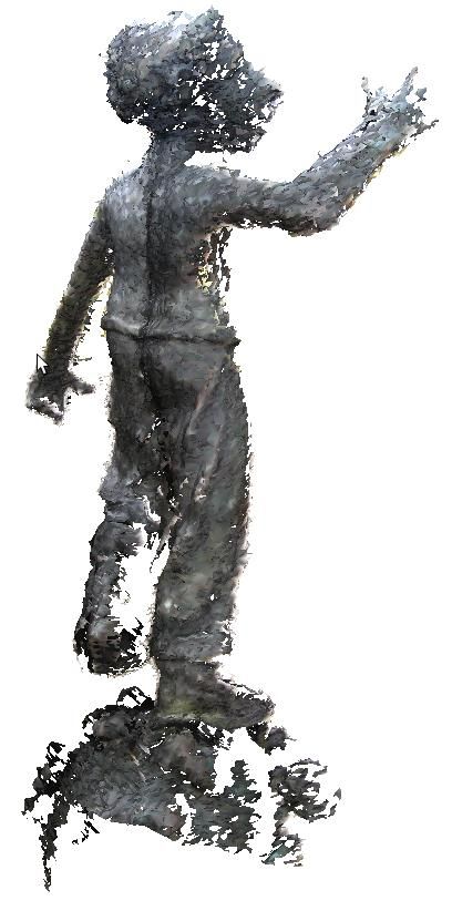
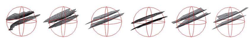
Hough Transforms and 3D SURF for robust three dimensional classification                    5

Fig. 3. Each row shows some partial 3D shapes from which features were computed
that belong to the same visual word. The feature center is represented as a red dot,
while the sphere represents the feature scale. Each shape is shown normalized with
respect to the scale of the feature.

on whether the query shape’s center is already known, the above information is
used for classification in two ways as outlined in § 3.3.

3.1    Visual Vocabulary Construction

To reduce the dimensionality of feature matching and limit the effects of noise, we
quantize the SURF features to a vocabulary of visual words, which we define as
the cluster centers of an approximate K-means algorithm (see Muja et al. [18]).
Following standard practice [19, 20] in large-scale image searching, we set the
number of visual words (clusters) to 10% of the total number of features in
our training set. In practice, this yields a reasonable balance between mapping
similar shapes to the same visual word (Fig. 3) while ensuring that features that
are assigned the same word are indeed likely to correspond (Fig. 4).

3.2    Learning and Weighting Votes

Rather than storing a shape for each class, the ISM-based methods keep track
of where a visual word v would be located on a shape of class c relative to c’s
center ([16, 21]). This information — the collection of visual words and offsets
from shape centers — is assembled from the training set, and stored along with
the visual words themselves. Word v is therefore associated with a list of votes,
each of those being generated from a feature (introduced in Eq. 2) and defined
by the feature’s class c, its vector to the shape center (x0 , y 0 , z 0 ), its scale σ 0 , and
the scale of the shape. Each word may therefore cast votes for multiple classes.
Words may also cast multiple votes for the same class, as in Fig. 5, because there
may be multiple features on a shape associated with the same visual word.
6        J. Knopp, M. Prasad, G. Willems, R. Timofte, L. Van Gool

    Fig. 4. Examples of visual vocabulary based correspondences between 3D shapes.

    Suppose now that a query shape contains a feature at location [x, y, z]T with
scale σ that is assigned to visual word v. That feature will cast a vote, λ, for a
shape of class c centered at location
                 h                                                            iT
            λ = x − x0 (σ/ σ 0 ), y − y 0 (σ/ σ 0 ), z − z 0 (σ/ σ 0 ), σ/ σ 0 , (3)

with relative shape size σ/ σ 0 . If the query shape exactly matches a training
shape, the votes associated with that training shape will all be cast at the query
shape’s center, making a strong cluster of votes for the match. On the other
hand, the votes associated with a training shape from a different class will get
scattered around, because the spatial arrangement of features (and therefore
visual words) will be different, see Fig. 5.
    Note that although a single assignment of features to the closest visual word
is natural, it is subject to noise when cluster centers are close together. Therefore,
during the training phase, each feature activates the closest word and every other
word within a distance τ , as in [16, 20, 22]. This ensures that similar visual words
that are located at the same position on a shape will all vote appropriately.
    An issue is that different classes may have different numbers of features, and
not all features discriminate equally well between classes. We account for these
next discuss factors with a pair of weights,
 (i) a statistical weight Wst as every vote should be invariant to the number of
     training samples in the class,
(ii) a learned weight Wlrn weights every vote so it correctly votes for a class
     centre across training shapes.

(i) The statistical weight Wst (ci , vj ) weights all the votes cast by visual word
vj for class ci by
                                                                           nvot (ci ,vj )
                                         1               1                  n     (c )
                   Wst (ci , vj ) =   nvw (ci )   ·   nvot (vj )   ·    X nf tr (ci ,v )     ,   (4)
                                                                               vot k j
                                                                               nf tr (ck )
                                                                       ck ∈C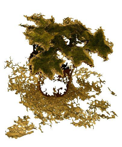
Hough Transforms and 3D SURF for robust three dimensional classification               7

Fig. 5. Example of the votes cast from four features on a cat shape instance. All
detected features are visualized as small black dots and votes are shown as lines starting
from the feature (marked blue). The votes from a toy ISM model were learned from
six shapes of the cat-class (visualized as green lines) and six shapes of flamingo-class
(red lines).

where the different numbers n are determined from the training set. For instance,
nvot (vj ) is the total number of votes from visual word vj , nvot (ci , vj ) is the
number of votes for class ci from vj , nvw (ci ) is the number of visual words that
vote for class ci , nf tr (ci ) is the number of features from which ci was learned. C is
the set of all classes. The first term makes every class invariant to the number
of visual words in its training set, while the second normalizes for the number of
votes each visual word casts. The final term reflects the probability that vj votes
for class ci as opposed to some other class.

(ii) Additionally, motivated by Maji’s et al. [23] work, we normalize votes on
the basis of how often they vote for the correct training shape centers (during
training). We define λij as the vote cast by a particular instance of visual word
vj on a particular training shape of class ci ; that is, λij records the distance of
the particular instance of visual word vj to the center of the training shape on
which it was found. We now apply this vote to every instance of visual word
vj on every training shape in class ci , and compute a Gaussian function of the
distance between the center position voted for and the actual center. This scheme
puts more emphasis on features with voted positions close to that actual center.
    For every vote λij , our goal is to obtain one value summarizing the statistics
of distances to shape centers,
                                                  da (λij )2
                                                                      !
                                               −
                     Wlrn (λij ) = f       e           σ2       a∈A        ,          (5)

where A is the set of all features associated with word vj on a shape of class ci
and da (λij ) is the Euclidean distance as just defined. We use a standard deviation
of σ taken as 10% of the shape size, which defines the accepted amount of noise.
For the function f , we observed the best performance for the median.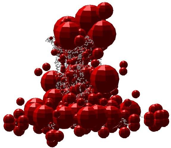
8            J. Knopp, M. Prasad, G. Willems, R. Timofte, L. Van Gool

                                           Visual                    Implicit Shape
                                         vocabulary                      Model

                  3D SURF                    indexing                   voting                              search

    query model             model+features              quanitzed features            probabilistic votes            recognized class

Fig. 6. Overview of our 3D ISM class recognition. On the query shape, 3D SURF
features are detected, described and quantized into the visual vocabulary. Using the
previously trained 3D Implicit Shape Model, each visual word then generates a set
of votes for the position of the class center and the relative shape size. Finally, the
recognized class is found at the location with maximum density of these votes.

       The final weight is the combination of Wst and Wlrn ,
                                      W (λij ) = Wst (vj , ci ) · Wlrn (λij ).                                                     (6)

3.3        Determining a Query Shape’s Class
The class recognition decision for a given 3D query shape is determined by the
set of 5D votes (shape center, size of the shape and class), weighted by the
function W . However, we need a mechanism to cluster votes cast at nearby but
distinct locations. Depending on the type of query shape, we use one of two
approaches:
 1. Cube Searching (CS): In the spirit of Leibe et al. [16], we discretize the
    5D search space into bins; each vote contributes to all bins based on its
    Gaussian-weighted distance to them. The recognized class and shape center
    is given by the highest score. The principal advantage of this approach is
    that it does not require a clean query shape — noisy or partial query input
    is handled by explicitly searching for the optimal shape center as well as the
    class.
 2. Distance to Shape Center (DC): Unlike image queries, where the shape’s
    center within the image is usually unknown, it is quite easy to compute the
    centroid of a clean 3D shape, and use this as the shape center. Doing so can
    simplify class recognition and improve its robustness by reducing the search
    to the best class given this center. We do this by weighting each vote by
    a Gaussian of its distance to the query shape’s center. Processing of such
    complete 3D shapes is a popular task in the 3D literature [11, 10]. Obviously,
    the real object center coinciding with the shape center is not always valid
    and we cannot use it for partial shapes or for the recognition of 3D scenes
    (with additional clutter or noise).

4        Experiments and Applications
Our main target is to robustly classify 3D shapes. Having visually assessed the
3D SURF descriptors (§ 2) in Figs. (3,4), we evaluate it further for the difficult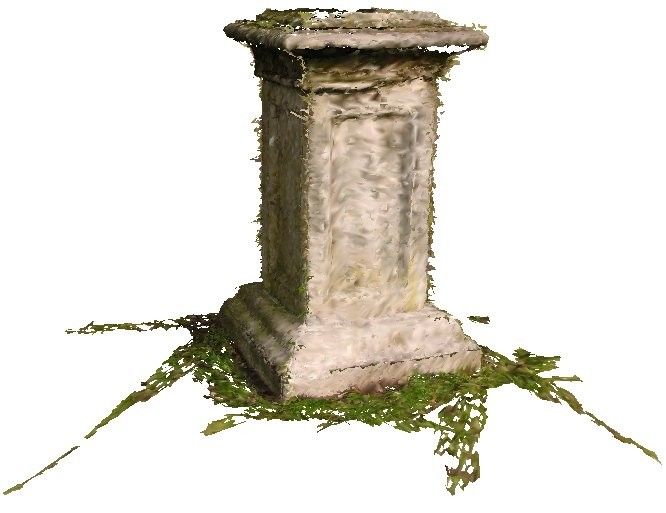
Hough Transforms and 3D SURF for robust three dimensional classification           9

task of partial shape retrieval in § 4.2. Since the task is retrieval, the features are
used in the BOF framework for this test. Supported by the good performance,
we further use 3D SURF features in conjunction with the probabilistic Hough
voting method of § 3 (ISM) to demonstrate its power for class recognition and
for assessing the sensitivity to missing data on standard datasets. Our proposed
method outperforms the other approaches in these clean shape datasets. Finally,
we tackle classification of 3D scenes reconstructed from real life images. Such
scenes are challenging due to clutter, noise and holes. We show promising results
on such data in § 4.4.

4.1   Datasets

All the datasets (Fig. 9) used in our evaluations consists of clean and segmented
shapes and are defined at the outset.

  (i) KUL dataset: simple dataset of 94 training shapes of 8 classes from the
      Internet and 22 query shapes.
 (ii) Princeton dataset: challenging dataset of 1.8K shapes (half training, half
      testing), 7 classes taken from the Princeton Benchmark [24].
(iii) Tosca+Sumner dataset: dataset for retrieval/classification [25, 26] of 474
      shapes, 12 classes of which 66 random ones form a test set.
(iv) SHREC’09 datasets: 40 classes, 720 training and 20 partial query shapes
      from the Partial Shape Retrieval Contest [27] with complete ground-truth.

4.2   3D SURF features for shape retrieval

We have presented a novel method for local features extraction and descrip-
tion for 3D shapes. We investigate now the performance of our approach to the
state of the art descriptors.
    As the task here is that of shape retrieval (as opposed to our classification
based method from § 3), we use 3D SURF features in the large-scale image re-
trieval approach of Sivic and Zisserman [19] based on BOF. First, 3D SURF
features of all shapes were quantized using the visual vocabulary as in § 3. Sec-
ond, we compute the BOF vectors. Third, using the BOF, every shape model
is represented as the normalized tf-idf vector [28] preferring the discriminative
visual words. Finally, the similarity between shapes is measured as the L1 dis-
tance between the normalized tf-idf vectors. L1 measure was shown to perform
better than the dot-product in image retrieval [19].
    For the problem of partial shape retrieval 3D SURF is pitched against other
descriptors in the SHREC’09 Contest [27] for the dataset (iv) in § 4.1. Fig. 7(a)
presents our results together with results from the SHREC’09 Contest. Note that
3D SURF features outperform the rendered range-images -based SIFT descrip-
tors [27], in similar BOF frameworks.
    Fig. 7(b,c) shows the retrieval performance on two additional datasets. As
the main result, we observed high sensitivity of all descriptors to to the dataset
10                            J. Knopp, M. Prasad, G. Willems, R. Timofte, L. Van Gool

                     0.6                                                                                  BOF−our 3DSURF
                                                                                                          BOF−Sun’s HKS
                                                                                                          BOF−Jonson’s SI
                     0.4                                                                                  BOF−Kobbelt’s SH
      Precision                                                                                           BOF−Osada’s shapeD2
                                                                                                          Random
                                                                                                          Daras: CMVD Binary
                     0.2                                                                                  Daras: CMVD Depth
                                                                                                          Daras: Merged CMVD−Depth
                                                                                                          and CMVD−Binary
                              0                                                                           Furuya: BOF−SIFT
                                  0        0.2          0.4       0.6              0.8             1      Furuya: BOF−GRID−SIFT
                                                           Recall
                                                (a) SHREC’09 dataset
                                  1                                                      1

                              0.8                                                       0.8
                  Precision

                                                                            Precision
                              0.6                                                       0.6

                              0.4                                                       0.4

                              0.2                                                       0.2

                                  0                                                      0
                                      0   0.2      0.4      0.6   0.8   1                     0   0.2   0.4      0.6   0.8     1
                                                      Recall                                               Recall
                         (b) Tosca, small resolution shapes                                       (c) KUL dataset

Fig. 7. Comparison of different detectors/descriptors using the video google [19]
retrieval approach. The performance is measured as Precision-Recall curve.
(a) SHREC’09 Partial Shape Retrieval Contest [27] provided results which were com-
pared with our 3D SURF and other approaches. (b,c) Note that the performance highly
depends on the shape’s type as results very depend on dataset.

type, i.e. SI [15] outperforms all methods in Tosca dataset, while it gives the
worst results on KUL dataset, but couldn’t be evaluated on SHREC’09 due to
computational constraints.
   We also observed (on shapes from 1.2K-65K faces and 670-33K vertices) that
our method is faster than other local descriptors. In average, 3D SURF takes
20.66s, HKS [6] 111.42s and SI [15] more than 15mins. The experiment was
performed on 4xQuad Core AMD Opteron, 1.25Ghz/core.

4.3                3D SURFs in the ISM framework for 3D classification
Here we apply our method (ISM, § 3) for shape classification in these variations:
(a) ISM-CS: with the cube-searching method from § 3.3 (1).
(b) ISM-DC: with the assumption that the shape’s centre is known (see § 3.3 (2)).
The above versions of our method are compared against the following:
(i) BOF-knn: Encouraged by the good results of the 3D shape retrieval al-
    gorithm in § 4.2, we use this as one competitor. The test query shape is
    assigned to the most commonly occurring class of the best k-retrieved train-
    ing shapes in a nearest-neighbor classification approach. Parameter k was
Hough Transforms and 3D SURF for robust three dimensional classification 11
100
classification performance [%]
Fig. 8. Sensitivity
of 3D classification
90
to missing data.
The classification
80
performance is plot-
70
ted as the shape is
3D SURF, ISM−DC increasingly cropped.
60
3D SURF, ISM−CS See the fish example
3D SURF, BOF−knn
3D SURF, Toldo−BOF−SVM
on the bottom row.
50 We found that our
0 10 20 30 40 50 60 70 80
approach outper-
erased part of shape [%]
forms knn as well
as Toldo’s [11] SVM
method.
learnt to optimize classification of train shapes. The shapes are represented
by normalized tf-idf vectors and L1 is used as metric.
(ii) Toldo-BOF-SVM: This is our implementation of Toldo et al. [11], where
BOF vectors are computed on the training data MT . Then, the multi-class
SVM classifier ([29]) is learned on the BOF vectors to predict the class label
of the query shapes MQ . The kernel function is defined in terms of histogram
intersection as in [11].
First, we investigate the sensitivity of classification methods with respect
to the occlusions. Fig. 8 shows the performance of methods in the presence of
occlusion on KUL dataset (§ 4.1 (i)). ISM-DC gives the best results for complete
models and the performance of ISM-CS outperforms all methods with the more
partial queries.
Table 1 summarizes all results on standard datasets of 3D shapes. Here, we
measured the performance of classification methods on several datasets. Our
approach using the Hough voting gave the average performance (see the last
column in Table 1). The Princeton dataset (§ 4.1 (ii)) is the most challenging
and although all methods gave similar results, we outperform the others. This
dataset has very high variation amongst its 3D models i.e. the animal class
contains widely varying models of ’ant’ and ’fish’. For an SVM to learn a good
classifier, we need a good non-linear kernel which has learnt such differences
well. In such cases, non-parametric nearest-neighbor classifiers have a natural
advantage.
The SHREC’09 dataset (§ 4.1 (iv)), previously used for the retrieval of partial
queries, is now used for classification. ISM doesn’t perform well as this method
needs relatively large number of training examples [16, 21] which is not satisfied
in this case.
We conclude that our ISM based method beats k-nn and SVM in most cases.12 J. Knopp, M. Prasad, G. Willems, R. Timofte, L. Van Gool
Princeton:
Tosca+Sumner:
SHREC’09:
Fig. 9. Samples of query shapes from the state-of-the-art datasets.
Princeton Tosca+Sumner SHREC’09
method # TP # FP perfor. # TP # FP perfor. # TP # FP perfor. avg. perf.
ISM 529 378 58.3% 56 1 98% 8 14 40% 65.4%
BOF-knn 491 416 54.1% 56 1 98% 7 13 35% 62.4%
BOF-SVM 472 435 52.0% 41 16 72% 12 8 60% 61.3%
Table 1. Table summarizes all results of classification on state-of-the-art datasets.
Proposed approach beats k-nn and SVM in most cases.
4.4 3D shape classification of reconstructed real life scenes
As a final note, it is interesting to investigate the relative roles 2D and 3D object
class detection could play in real-life. We carry out a small experiment to see
whether 3D detection would really offer an added value.
Given many images taken in uncontrolled conditions around a real object,
state-of-the-art methods such as the Arc3D web-service [30] can be used to
extract a dense 3D model from the captured images. Such object models exhibit
varying amounts of noise, holes and clutter from the surroundings, as can be
seen from the examples (see Fig. 10). For each class on Fig. 10 we reuse the 3D
ISM models trained on datasets of the SHREC’09 (for bike and plant classes),
Tosca+Sumner (for woman) and KUL (for cube and people). We also used 2D
Felzenszwalb detectors [31] trained on data from the PASCAL’08 datasets for
bikes, potted plants, and pedestrians. As shown in the Fig. 10, a small test was
run, where 3D reconstructions were produced from images for an instance of
each of the 6 objects. In each of these cases, the classification using 3D ISM was
successful, while SVM based method of Toldo et al. [11] failed in all cases. As
to the 2D detectors, the bike was found in 12 out of the 15 images, the potted
plant in none of the 81 images, and the person in 47 out of the hundred. This
would indicate that given a video images input, a single 3D detection into the
images could be more effective than 2D detections in separate images. But issues
concerning 2D vs. 3D detection need to be explored further.
5 Conclusion
In this paper, we introduced 3D SURF features in combination with the proba-
bilistic Hough voting framework for the purpose of 3D shape class recognition.Hough Transforms and 3D SURF for robust three dimensional classification 13
people: 11 out of 33 woman: 47 out of 100
plant: 0 out of 81
bike: 12 out of 15
people: 18 out of 18
cube: n/a
Fig. 10. 3D class recognition from the set of images. For each sample: correctly recog-
nized class using 3D ISM, the number of correctly recognized objects in images using
the method of Felzenszwalb et al. [31] (the best for PASCAL’08), samples of detection
results are highlighted by squares, and the reconstructed shape by Arc3D [30].
This work reaffirms the direction taken by recent research in 2D class detection,
but thereby deviates rather strongly from traditional 3D approaches, which are
often based on global features, and where only recently some first investigations
into local features combined with bag-of-features classification were made.
We have demonstrated through experiments, first the power of the features
(§ 4.2), followed by the combined power of the features and the classification
framework (§ 4.3). This method outperforms existing methods and both aspects
seem to play a role in that.
Acknowledgment. We are grateful for financial support from EC Integrated
Project 3D-Coform.
References
1. Kobbelt, L., Schrder, P., Kazhdan, M., Funkhouser, T., Rusinkiewicz, S.: Rotation
invariant spherical harmonic representation of 3d shape descriptors. (2003)
2. Saupe, D., Vranic, D.V.: 3d model retrieval with spherical harmonics and moments.
In: DAGM-Symposium on Pattern Recognition. (2001)
3. Osada, R., Funkhouser, T., Chazelle, B., Dobki, D.: Shape distributions. ACM
Transactions on Graphics (2002) 807–832
4. Leymarie, F.F., Kimia, B.B.: The shock scaffold for representing 3d shape. In:
Workshop on Visual Form (IWVF4). (2001)
5. Mian, A.S., Bennamoun, M., Owens, R.: Three-dimensional model-based object
recognition and segmentation in cluttered scenes. IEEE PAMI 28 (2006)
6. Sun, J., Ovsjanikov, M., Guibas, L.: A concise and provably informative multi-scale
signature based on heat diffusion. In: SGP. (2009) 1383–139214 J. Knopp, M. Prasad, G. Willems, R. Timofte, L. Van Gool
7. Gelfand, N., Mitra, N.J., Guibas, L.J., Pottmann, H.: Robust global registration.
In: Symposium on Geometry Processing. (2005) 197–206
8. Pottmann, H., Wallner, J., Huang, Q.X., Yang, Y.L.: Integral invariants for robust
geometry processing. Comput. Aided Geom. Des. 26 (2009) 37–60
9. Novatnack, J., Nishino, K.: Scale-dependent/invariant local 3d shape descriptors
for fully automatic registration of multiple sets of range images. In: ECCV. (2008)
10. Ovsjanikov, M., Bronstein, A.M., Bronstein, M.M., Guibas, L.J.: Shapegoogle: a
computer vision approach for invariant shape retrieval. (2009)
11. Toldo, R., Castellani, U., Fusiello, A.: A bag of words approach for 3d object
categorization. In: MIRAGE. (2009)
12. Golovinskiy, A., Kim, V.G., Funkhouser, T.: Shape-based recognition of 3d point
clouds in urban environments. In: ICCV. (2009)
13. Brostow, G.J., Shotton, J., Fauqueur, J., Cipolla, R.: Segmentation and recognition
using structure from motion point clouds. In: ECCV (1). (2008)
14. Bay, H., Ess, A., Tuytelaars, T., Van Gool, L.: Speeded-up robust features (surf).
Comput. Vis. Image Underst. 110 (2008) 346–359
15. Johnson, A.E., Hebert, M.: Using spin images for efficient object recognition in
cluttered 3d scenes. IEEE PAMI 21 (1999) 433–449
16. Leibe, B., Leonardis, A., Schiele, B.: Robust object detection with interleaved
categorization and segmentation. IJCV 77 (2008) 259–289
17. Willems, G., Tuytelaars, T., Van Gool, L.: An efficient dense and scale-invariant
spatio-temporal interest point detector. In: ECCV. (2008) 650–663
18. Muja, M., Lowe, D.: Fast approximate nearest neighbors with automatic algorithm
configuration. In: VISAPP. (2009)
19. Sivic, J., Zisserman, A.: Video Google: A text retrieval approach to object matching
in videos. In: ICCV. (2003)
20. Jégou, H., Douze, M., Schmid, C.: Improving bag-of-features for large scale image
search. IJCV (2010) to appear.
21. Lehmann, A., Leibe, B., , Gool, L.V.: Feature-centric efficient subwindow search.
In: ICCV. (2009)
22. Philbin, J., Chum, O., Isard, M., Sivic, J., Zisserman, A.: Lost in quantization:
Improving particular object retrieval in large scale image databases. In: CVPR.
(2008)
23. Maji, S., Malik, J.: Object detection using a max-margin hough transform. In:
CVPR. (2009) 1038–1045
24. Shilane, P., Min, P., Kazhdan, M., Funkhouser, T.: The princeton shape bench-
mark. In: Shape Modeling International. (2004)
25. Bronstein, A., Bronstein, M., Kimmel, R.: Numerical Geometry of Non-Rigid
Shapes. Springer Publishing Company, Incorporated (2008)
26. Sumner, R.W., Popovic, J.: Deformation transfer for triangle meshes. ACM Trans.
Graph. 23 (2004) 399–405
27. Dutagaci, H., Godil, A., Axenopoulos, A., Daras, P., Furuya, T., R. Ohbuchi, R.:
Shrec 2009 - shape retrieval contest of partial 3d models. (2009)
28. Salton, G., Buckley, C.: Term-weighting approaches in automatic text retrieval.
Inf. Process. Manage. 24 (1988) 513–523
29. Chang, C.C., Lin, C.J.: LIBSVM: a library for support vector machines. (2001)
Software available at http://www.csie.ntu.edu.tw/~cjlin/libsvm.
30. Vergauwen, M., Gool, L.V.: Web-based 3d reconstruction service. Mach. Vision
Appl. 17 (2006) 411–426
31. Felzenszwalb, P.F., Girshick, R.B., McAllester, D., Ramanan, D.: Object detection
with discriminatively trained part based models. IEEE PAMI 99 (2009)You can also read