Manipulating Highly Deformable Materials Using a Visual Feedback Dictionary
←
→
Page content transcription
If your browser does not render page correctly, please read the page content below
Manipulating Highly Deformable Materials Using a Visual Feedback
                                                                          Dictionary
                                                                                  Biao Jia, Zhe Hu, Jia Pan, Dinesh Manocha
                                                                                 http://gamma.cs.unc.edu/ClothM/

                                            Abstract— The complex physical properties of highly de-
                                         formable materials such as clothes pose significant challenges
                                         fanipulation systems. We present a novel visual feedback
                                         dictionary-based method for manipulating defoor autonomous
arXiv:1710.06947v3 [cs.RO] 16 Jan 2019

                                         robotic mrmable objects towards a desired configuration. Our
                                         approach is based on visual servoing and we use an efficient
                                         technique to extract key features from the RGB sensor stream
                                         in the form of a histogram of deformable model features. These
                                         histogram features serve as high-level representations of the
                                         state of the deformable material. Next, we collect manipulation
                                         data and use a visual feedback dictionary that maps the velocity
                                         in the high-dimensional feature space to the velocity of the
                                         robotic end-effectors for manipulation. We have evaluated our
                                         approach on a set of complex manipulation tasks and human-
                                         robot manipulation tasks on different cloth pieces with varying
                                         material characteristics.

                                                                I. I NTRODUCTION                                 Fig. 1: Manipulation Benchmarks: We highlight the real-time
                                            The problem of manipulating highly deformable materials              performance of our algorithm on three tasks: (1) human-robot
                                                                                                                 jointly folding a cloth with one hand each; (2) robot folding a
                                         such as clothes and fabrics frequently arises in different ap-          cloth with two hands; (3) human-robot stretching a cloth with four
                                         plications. These include laundry folding [1], robot-assisted           combined hands. The top row shows the initial state for each task
                                         dressing or household chores [2], [3], ironing [4], coat                and the bottom row is the final state. Our approach can handle the
                                         checking [5], sewing [6], and transporting large materials              perturbations due to human movements.
                                         like cloth, leather, and composite materials [7]. Robot ma-             on appropriate low-dimensional features. Current methods
                                         nipulation has been extensively studied for decades and                 may not work well while performing complex tasks or when
                                         there is extensive work on the manipulation of rigid and                the model undergoes large deformations. Furthermore, in
                                         deformable objects. Compared to the manipulation of a rigid             many human-robot systems, the deformable material may
                                         object, the state of which can be completely described by a             undergo unknown perturbations and it is important to design
                                         six-dimensional configuration space, the manipulation of a              robust manipulation strategies [3], [10].
                                         deformable object is more challenging due to its very high              Main Results: In this paper, we present a novel feature
                                         configuration space dimensionality. The resulting manipula-             representation, a histogram of oriented wrinkles (HOW), to
                                         tion algorithm needs to handle this dimensional complexity              describe the shape variation of a highly deformable object
                                         and maintain the tension to perform the task.                           like clothing. These features are computed by applying
                                            One practical approach to dealing with general deformable            Gabor filters and extracting the high-frequency and low-
                                         object manipulation is based on visual servoing, [8], [9]. At           frequency components. We precompute a visual feedback
                                         a broad level, these servoing techniques use perception data            dictionary using an offline training phase that stores a
                                         captured using cameras and formulate a control policy map-              mapping between these visual features and the velocity of
                                         ping to compute the velocities of the robotic end-effectors             the end-effector. At runtime, we automatically compute the
                                         in real-time. However, a key issue in these methods is to               goal configurations based on the manipulation task and use
                                         automatically extract key low-dimensional features of the               sparse linear representation to compute the velocity of the
                                         deformable material that can be used to compute a mapping.              controller from the dictionary (Section III). Furthermore,
                                         The simplest methods use manual or other techniques to                  we extend our approach so that it can be used in human-
                                         extract features corresponding to line segments or curvature            robot collaborative settings. Compared to prior manipulation
                                         from a set of points on the surface of the deformable material.         algorithms, the novel components of our work include:
                                         In addition, we need appropriate mapping algorithms based
                                                                                                                   •   A novel histogram feature representation of highly
                                           Biao Jia and Dinesh Manocha are with the Department of Computer             deformable materials (HOW-features) that are computed
                                         Science, University of North Carolina at Chapel Hill. E-mail: {biao,          directly from the streaming RGB data using Gabor
                                         dm}@cs.unc.edu.
                                           Zhe Hu and Jia Pan are with the Department of Mechanical Biomedical         filters (Section IV).
                                         Engineering, City University of Hong Kong.                                •   A sparse representation framework using a visual feed-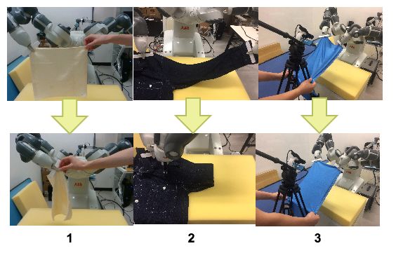
m                   state of the deformable object
      back dictionary, which directly correlates the histogram      r                   robot’s end-effector configuration
      features to the control instructions (Section V).             v                   robot’s end-effector velocity, v = ṙ
   • The combination of deformable feature representation,          I(w, h)             image from the camera, of size (wI , hI )
                                                                    s(I)                HOW-feature vector extracted from image I
      a visual feedback dictionary, and sparse linear represen-     di (I)              the i-th deformation kernel filter
      tations that enable us to perform complex manipulation        I (t) , r(t)        time index t of images and robot configurations
      tasks, including human-robot collaboration, without sig-      {∆s(i) },{∆r(i) }   features and labels of the visual feedback dictionary
      nificant training data (Section V-C).                         ρ(·, ·)             error function between two items
                                                                    λ                   positive feedback gain
We have integrated our approach with an ABB YuMi dual-              L                   interaction matrix linking velocities of the feature
arm robot and a camera for image capture and used it                                    space to the end-effector configuration space
                                                                    F                   interaction function linking velocities of the feature
to manipulate different cloth materials for different tasks.                            space to the end-effector configuration space
We highlight the real-time performance for tasks related to         pj (i)              jth histogram of value i
stretching, folding, and placement (Section VI).                    Ndof,I,r,d          number of degrees of freedom of the manipulator
                                                                                        images {I (t) }, samples {r(t) } ,filters {d(t) }
                    II. R ELATED W ORK                              Cf r                constant of frame rate
                                                                    r ∗ , s ∗ , m∗      desired target configuration, feature, state
   Many techniques have been proposed for the automated             r̂, ŝ, m̂          approximated current configuration, feature, state
manipulation of flexible materials. Some of them have been                           TABLE I: Symbols used in the paper
designed for specific tasks, such as peg-in-hole and laying
                                                                   techniques for folding clothes. Cusumano-Towner et al. [21]
down tasks with small elastic parts [11] or wrapping a cloth
                                                                   learn a Hidden Markov Model (HMM) using a sequence of
around a rigid surface [12]. There is extensive work on
                                                                   manipulation actions and observations.
folding laundry using pre-planned materials. In this section,
we give a brief review of prior work on deformable object          C. Visual Servoing for Deformable Objects
representation, manipulation, and visual servoing.                    Visual servoing techniques [22], [23] aim at controlling a
A. Deformable Object Representation                                dynamic system using visual features extracted from images.
                                                                   They have been widely used in robotic tasks like manip-
   The recognition and detection of deformable object char-        ulation and navigation. Recent work includes the use of
acteristics is essential for manipulation tasks. There is exten-   histogram features for rigid objects [24]. Sullivan et al. [13]
sive work in computer vision and related areas on tracking         use a visual servoing technique to solve the deformable
features of deformable models. Some of the early work is           object manipulation problem using active models. Navarro-
based on active deformable models [13]. Ramisa et al. [14]         Alarcon et al. [8], [9] use an adaptive and model-free linear
identify the grasping positions on a cloth with many wrinkles      controller to servo-control soft objects, where the object’s
using a bag-of-features-based detector. Li et al. [15] encode      deformation is modeled using a spring model [25]. Langsfeld
the category and pose of a deformable object by collecting         et al. [26] perform online learning of part deformation
a large set of training data in the form of depth images from      models for robot cleaning of compliant objects. Our goal is
different view points using offline simulation.                    to extend these visual servoing methods to perform complex
B. Deformable Object Manipulation                                  tasks on highly deformable materials.
   Robotic manipulation of general deformable objects relies                                  III. OVERVIEW
on a combination of different sensor measurements. The                In this section, we introduce the notation used in the
RGB images or RGB-Depth data are widely used for de-               paper. We also present a formulation of the deformable object
formable object manipulation [1], [4], [9]. Fiducial markers       manipulation problem. Next, we give a brief background on
can also be printed on the deformable object to improve the        visual servoing and the feedback dictionary. Finally, we give
manipulation performance [16]. In addition to visual percep-       an overview of our deformable manipulation algorithm that
tion, information from other sensors can also be helpful, like     uses a visual feedback dictionary.
the use of contact force sensing to maintain the tension [7]. In
many cases, simulation techniques are used for manipulation        A. Problem Formulation
planning. Clegg et al. [17] use reinforcement learning to train       The goal of manipulating a highly deformable material is
a controller for haptics-based manipulation. Bai et al. [18]       to drive a soft object towards a given target state (m∗ ) from
use physically-based optimization to learn a deformable ob-        its current state (m). The state of a deformation object (m)
ject manipulation policy for a dexterous gripper. McConachie       can be complex due to its high dimensional configuration.
et al. [19] formulate model selection for deformable object        In our formulation, we do not represent this state explicitly
manipulation and introduces a utility metric to measure the        and treat it as a hidden variable. Instead, we keep track of
performance of a specific model. These simulation-based            the deformable object’s current state in the feature space (s)
approaches need accurate deformation material properties,          and its desired state (s∗ ), based on HOW-features.
which can be difficult to achieve. Data-driven techniques             The end-effector’s configuration r is represented using the
have been used to design the control policies for deformable       Cartesian coordinates and the orientations of end-effectors or
object manipulation. Yang et al. [20] propose an end-to-           the degree of each joint of the robot. When r corresponds to
end framework to learn a control policy using deep learning        the Cartesian coordinates of the end-effectors, an extra step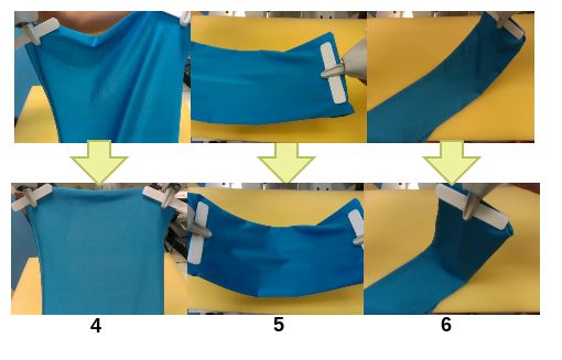
Fig. 2: Computing the Visual Feedback Dictionary: The input to
this offline process is the recorded manipulation data with images     Fig. 3: Runtime Algorithm: The runtime computation consists
and the corresponding configuration of the robot’s end-effector. The   of two stages. We extract the deformable features (HOW-features)
output is a visual feedback dictionary, which links the velocity of    from the visual input and computes the visual feedback word by
the features and the controller.                                       subtracting the extracted features from the features of the goal
                                                                       configuration. We apply the sparse representation and compute the
                                                                       velocity of the controller for manipulation.
is performed by the inverse kinematics motion planner [27]
to map the velocity v to the actual controlling parameters.            is equivalent to minimizing the Euclidean distance in the
   The visual servo-control is performed by computing an               feature space and this can be expressed as:
appropriate velocity (v) of the end-effectors. Given the visual
feedback about the deformable object, the control velocity                       rˆ∗ = arg min((s(r) − s∗ )T (s(r) − s∗ )),         (3)
                                                                                           r
(v) reduces the error in the feature space (s − s∗ ). After
continuously applying feedback control, the robot will ma-             where s∗ = s(r∗ ) is the HOW-feature corresponding to the
nipulate the deformable object toward its goal configuration.          goal configuration (r∗ ). The visual servoing problem can
In this way, the feedback controller can be formulated as              be solved by iteratively updating the velocity of the end-
computing a mapping between the velocity in the feature                effectors according to the visual feedback:
space of the deformable object and the velocity in the end-                                                   ∗
                                                                                               v = −λL+
                                                                                                      s (s − s ),                   (4)
effector’s configuration space (r):
                                                                       where L+  s is the pseudo-inverse of the interaction matrix
                    r∗ − r = −λF (s − s∗ )                      (1)    Ls = ∂r∂s
                                                                                 . It corresponds to an interaction matrix that links
where F is an interaction function that is used to map the two         the variation of the velocity in the feature space ṡ to the
velocities in different spaces and λ is the feedback gain. This        velocity in the end-effector’s configuration space. L+
                                                                                                                            s can be

formulation works well only if some standard assumptions               computed offline by training data defined in [24].
related to the characteristics of the deformable object hold.          C. Visual Feedback Dictionary
These include infinite flexibility with no energy contribution
                                                                          The visual feedback dictionary corresponds to a set of
from bending, no dynamics, and being subject to gravity
                                                                       vectors with instances of visual feedback {∆s(i) } and the
and downward tendency (see details in [28]). For our tasks
                                                                       corresponding velocities of the end-effectors {∆r(i) }, where
of manipulating highly deformable materials like clothes or
                                                                       {∆s(i) } = (s − s∗ ). Furthermore, we refer to each in-
laundry at a low speed, such assumptions are valid.
                                                                       stance {∆s(i) , ∆r(i) } as the visual feedback word. This
B. Visual Servoing                                                     dictionary is computed from the recorded manipulation data.
   In this section we give a brief overview of visual servo-           The input includes a set of images ({I (t) }) and the end-
ing [22], [29], [24], [30], which is used in our algorithm. In         effector configurations ({r(t) }). Its output is computed as
general-purpose visual servoing, the robot wants to move an            ({{∆s(i) }, {∆r(i) }}). We compute this dictionary during
object from its original configuration (r) towards a desired           an offline learning phase using sampling and clustering
configuration (r∗ ). In our case, the object’s configuration           methods (see Algorithm 2 for details), and use this dictionary
(r) also corresponds to the configuration of the robot’s end-          at runtime to compute the velocity of the controller by
effector, because the rigid object is fixed relative to the end-       computing the sparse decomposition of a feedback ∆s. More
effectors during the manipulation task. These methods use a            details about computing the visual feedback dictionary are
cost function ρ(·, ·) as the error measurement in the image            give in Algorithm 2.
space and the visual servoing problem can be formulated as             D. Offline and Runtime Computations
an optimization problem:
                                                                          Our approach computes the visual dictionary using an
                     rˆ∗ = arg min ρ(r, r∗ ),                   (2)    offline process (see Fig. 2). Our runtime algorithm consists
                               r
                                                                       of two components. Given the camera stream, we extract the
where rˆ∗ is the configuration of the end-effector after the           HOW-features from the image (s(I)) and compute the cor-
optimization step and is the closest possible configuration to         responding velocity of the end-effector using an appropriate
the desired position (r∗ ). In the optimal scenario, rˆ∗ = r∗ .        mapping. For the controlling procedure, we use the sparse
   Let s be a set of HOW-features extracted from the image.            representation method to compute the interaction matrix,
Depending on the configuration r, the visual servoing task             as opposed to directly solving the optimization problem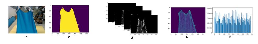
(Equation 2). In practice, the sparse representation method is    the position in the feature space of the deformation to achieve
more efficient. The runtime phase performs the actual visual      the manipulation task. Our approach is inspired by the study
servoing with the current image at time t (I (t) ), the visual    of grids of Histogram of Oriented Gradient [35], which is
feedback dictionary ({{∆s(i) }, {∆r(i) }}), and the desired       computed on a dense grid of uniformly spatial cells.
goal configurations given by (I ∗ ) as the input.                    We compute the grids of histogram of deformation model
                                                                  feature by dividing the image into small spatial regions and
  IV. H ISTOGRAM OF D EFORMATION M ODEL F EATURE
                                                                  accumulating local histogram of different filters (di ) of the
   In this section, we present our algorithm to compute           region. For each grid, we compute the histogram in the region
the HOW-features from the camera stream. These are low-           and represent it as a matrix. We vary the grid size and
dimensional features of the highly deformable material. The       compute matrix features for each size. Finally, we represent
pipeline of our HOW-feature computation process is shown          the entries of a matrix as a column feature vector. The
in Figure 4. Next, we explain each of these stages in detail.     complete feature extraction process is described in Algorithm
                                                                  1.
A. Foreground Segmentation
  To find the foreground partition of a cloth, we apply the       Algorithm 1 Computing HOW-Features
Gaussian mixture algorithm [31] on the RGB data captured
                                                                  Require: image I of size (wI , hI ), deformation filtering or
by the camera. The intermediate result of segmentation is
                                                                      Gabor kernels {d1 · · · dNd }, grid size set{g1 , · · · , gNg }.
shown in Figure 4(2).
                                                                  Ensure: feature vector s
B. Deformation Enhancement                                         1: for i = 1, · · · , Nd do
                                                                   2:   for j = 1, · · · , Ng do
    To model the high dimensional characteristics of the
                                                                   3:      for (w, h) = (1, 1), · · · , (wI , hI ) do
highly deformable material, we use deformation enhance-
                                                                   4:        (x, y) = (TRUNC(w/gj ), TRUNC(h/gj )) // com-
ment. This is based on the perceptual observation that
                                                                             pute the indices using truncation
most deformations can be modeled by shadows and shape
                                                                   5:        si,j,x,y = si,j,x,y + di (I(w, h)) //add the filtered
variations. Therefore, we extract the features corresponding
                                                                             pixel value to the specific bin of the grid
to shadow variations by applying a Gabor transform [32]
                                                                   6:      end for
to the RGB image. This results in the enhancement of the
                                                                   7:   end for
ridges, wrinkles, and edges (see Figure 4). We convolve the
                                                                   8: end for
N deformation filters {di } to the image I and represent the
                                                                   9: return s
result as {di (I)}.
    In the spatial domain, a 2D Gabor filter is a Gaussian
kernel function modulated by a sinusoidal plane wave [33]            The HOW-feature has several advantages. It captures the
and it has been used to detect wrinkles [34]. The 2D Gabor        deformation structure, which is based on the characteristics
filter can be represented as follows:                             of the local shape. Moreover, it uses a local representation
                                  2       2                       that is invariant to local geometric and photometric transfor-
                                 x0 + γ 2 y 0         x0
 g(x, y; λ, θ, φ, σ, γ) = exp(−          2
                                              ) sin(2π + φ),      mations. This is useful when the translations or rotations are
                                      2σ              λ           much smaller than the local spatial or orientation grid size.
                                                            (5)
where x0 = x cos θ + y sin θ, y 0 = −x sin θ + y cos θ, θ is
the orientation of the normal to the parallel stripes of the            V. M ANIPULATION USING V ISUAL F EEDBACK
Gabor filter, λ is the wavelength of the sinusoidal factor,                           D ICTIONARY
φ is the phase offset, σ is the standard deviation of the            In this section, we present our algorithm for computing
Gaussian, and γ is the spatial aspect ratio. When we apply        the visual feedback dictionary. At runtime, this dictionary
the Gabor filter to our deformation model image, the choice       is used to compute the corresponding velocity (∆r) of the
of wavelength (λ) and orientation (θ) are the key parameters      controller based on the visual feedback (∆s(I)).
with respect to the wrinkles of deformable materials. As a
result, the deformation model features consist of multiple
                                                                  A. Building Visual Feedback Dictionary
Gabor filters (d1···n (I)) with different values of wavelengths
(λ) and orientations (θ).                                            As shown in Figure 2, the inputs of the offline training
                                                                  phase are a set of images and end-effector configurations
C. Grids of Histogram                                             ({I (t) }, {r(t) }) and the output is the visual feedback dictio-
   A histogram-based feature is an approximation of the           nary ({{∆s(i) }, {∆r(i) }}).
image which can reduce the data redundancy and extract               For the training process, the end-effector configurations,
a high-level representation that is robust to local variations    ({r(t) }), are either collected by human tele-operation or
in an image. Histogram-based features have been adopted to        generated randomly. A single configuration (r(i) ) of the robot
achieve a general framework for photometric visual servo-         is a column vector of length Ndof , the number of degrees-
ing [24]. Although the distribution of the pixel value can be     of-freedom to be controlled. r ∈ RNdof and its value is
represented by a histogram, it is also significant to represent   represented in the configuration space.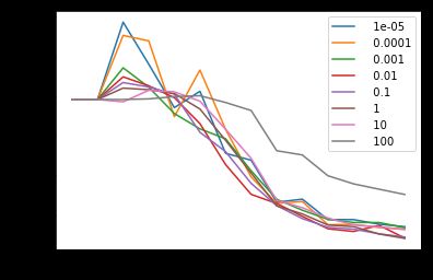
Fig. 4: Pipeline for HOW-feature Computation: We use the following stages for the input image (1): (2) Foreground segmentation
using Gaussian mixture; (3) Image filtering with multiple orientations and wavelengths of Gabor Kernel; (4) Discretization of the filtered
images to form grids of histogram; (5) Stacking the feature matrix to a single column vector.

   In order to compute the mapping (FH ) from the visual                            back dictionary. These representations tend to assign zero
feedback to the velocity, we need to transform the configura-                       weights to most irrelevant or redundant features and are used
tions {r(t) } and image stream {I (t) } into velocities {∆r(t) }                    to find a small subset of most predictive features in the high
and the visual feature feedback {∆s(t) }. One solution is to                        dimensional feature space. Given a noisy observation of a
select a fixed time step ∆t and to represent the velocity in
both the feature and the configuration space as:                                    feature at runtime (s) and the visual feedback dictionary
                                                                                    constructed by features {∆s(i) } with labels {∆r(i) }, we
            (t+ ∆t    )     (t− ∆t )                    (t+ ∆t   )        (i− ∆t  )                   ˆ which is a sparse linear combination of
          r       2     − r     2                   s(I        2 ) − s(I        2 )
                                                                                    represent ∆s by ∆s,
∆r(t) =                              ; ∆s(I (t) ) =                                       (i)
                  ∆t/Cf r                                       ∆t/Cf r             {∆s }, where β is the sparsity-inducing L1 term. To deal
 where Cf r is the frame rate of the captured video.                                with noisy data, we rather use the L2 norm on the data-fitting
    However, sampling by a fixed time step (∆t) leads to term and formulate the resulting sparse representation as:
a limited number of samples (NI − ∆t) and can result in                                                           X
over-fitting. To overcome this issue, we break the sequential                         β̂ = arg min(||min(∆s −         βi ∆s(i) )||22 + α||β||1 ), (6)
order of the time index to generate more training data from                                    β                   i
I (t) and r(t) . In particular, we assume the manipulation task
can be observed as a Markov process [36] and each step where α is a slack variable that is used to balance the trade-
is independent from every other. In this case, the sampling off between fitting the data perfectly and using a sparse
rates are given as follows, (when the total sampling amount solution. The sparse coefficient β ∗ is computed using a
is n):                                                                              minimization formulation:
                (pt )     (pt+n )                       (pt )         (pt+n )
              r        −r                           s(I       ) − s(I         )                                              (j)
                                                                                                     X             X                    X
  ∆r(t) =                           ; ∆s(I (t) ) =                                    β ∗ = arg min(     ρ(∆s∗i −      βj ∆si ) + α         ||βj ||1 )
           (pt − pt+n )/Cf r                     (pt − pt+n )/Cf r                        β        i               j                    j
 where p1,··· ,2n is a set of indices randomly generated, and                                                                         (7)
pt ∈ [1 · · · NI ]. In order to build a more concise dictionary,                                                    ˆ and the probable
                                                                             After β̂ is computed, the observation ∆s
we also apply K-Means Clustering [37] on the feature space,                         ˆ can be reconstructed by the visual feedback dictio-
                                                                             label ∆r
which enhance the performance and prevent the over-fitting                   nary :
problem.                                                                             ˆ =
                                                                                           X
                                                                                                           ˆ =
                                                                                                                 X
                                                                                    ∆s        β̂i ∆s(i)   ∆r         β̂i ∆r(i)        (8)
   In practice, the visual feedback dictionary can be regarded
                                                                                               i                           i
as an approximation of the interaction function F (see                                                  ∗
Equation 1). The overall algorithm to compute the dictionary                 The corresponding ∆r of the i−th DOF in the configuration
is given in Algorithm 2.                                                     is given as:
                                                                                                                (j)
                                                                                                      X
                                                                                               ∆ri∗ =     βj∗ ∆ri ,                (9)
B. Sparse Representation                                                                                       j
  At runtime, we use sparse linear representation [38] to                              (j)
compute the velocity of the controller from the visual feed-                 where   ∆si    denotes the i−th datum of the j−th feature
                                                                             , ∆s∗i denotes
                                                                                         P the value of the response, and the norm-1
                                                                             regularizer j ||βj ||1 typically results in a sparse solution
                                                                             in the feature space.
                                                                             C. Goal Configuration and Mapping
                                                                               We compute the goal configuration and the corresponding
                                                                             HOW-features based on the underlying manipulation task at
                                                                             runtime. Based on the configuration, we compute the velocity
                                                                             of the end-effector. The different ways to compute the goal
                                                                             configuration are:
Fig. 5: Visual Feedback Dictionary: The visual feedback word is
defined by the difference between the visual features ∆s = s − s∗              • For the task of manipulating deformable objects to a
and the controller positions ∆r = r − r∗ . The visual feedback                    single state m∗ , the goal configuration can be repre-
dictionary {{∆s(i) }, {∆r(i) }} consists of visual feedback words                 sented simply by the visual feature of the desired state
computed. We show the initial and final states on the left and right,             s∗ = s(I ∗ ).
respectively.
Algorithm 2 Building the Visual Feedback Dictionary
Require: image stream {I (t) } and positions of end-effectors
{r(t) } with sampling amount n, dictionary size Ndic
(i) (i)
Ensure: Visual Feedback Dictionary {{∆sd }, {∆rd }}
1: {∆sd } = {}, {∆rd } = {}
2: p = NI RAND (2n) // generate random indices for sam-
pling
3: for i = 1, · · · , n do
4: ∆s(i) = s(I (p(i)) ) − s(I (p(i+n)) ) // sampling
5: ∆r(i) = r(p(i)) − r(p(i+n)) // sampling
6: end for
Fig. 6: Manipulation Benchmarks: We highlight three bench-
7: centers = K-MEANS({∆s(i) }, Ndic ) // compute the
marks corresponding to: (4) flattening; (5) placement; (6) folding.
centers of the feature set for clustering Top Row: The initial state of each task. Bottom Row: The goal
8: for i = 1, · · · , Ndic do state of each task. More details are given in Fig. 11.
9: j = arg mini (centers[i] − s(i) )
10: {∆sd } = {∆sd , ∆s(j) } {∆rd } = {∆rd , ∆r(j) }
11: end for
12: return {∆sd }, {∆rd }
• For the task of manipulating deformable objects to a
hidden state h∗ , which can be represented by a set
of states of the object h∗ = {m1 , · · · , mn } as a set
of visual features {s(I1 ), · · · , s(In )}. We modify the
formulation in Equation 1 to compute v as:
v = −λ min(F (s(I) − s(Ij ))) (10)
i
• For a complex task, which can be represented using
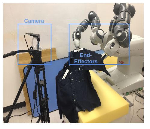
a sequential set of states {m1 , · · · , mn }, we estimate Fig. 7: Setup for Manipulation Tasks: We use an 12-DOF
the sequential cost of each state as c(mi ). We use a dual-arm ABB YuMi and an RGB camera to perform complex
modification that tends to compute the state with the manipulation tasks using visual servoing, with and without humans.
lowest sequential cost: A. Robot Setup and Benchmarks
∗ Our algorithm was implemented on a PC and integrated
i = arg min(c(mi ) − λF (s(I) − s(Ii ))). (11)
i with an ABB YuMi dual-arm robot with 12-DOF to capture
After i∗ is computed, the velocity for state mi is {r(t) } and perform manipulation tasks. We use a RealSense
determined by s(Ii∗ ), and mi is removed from the set camera is used to capture the RGB videos at (640 × 480)
of goals for subsequent computations. resolution. In practice, we compute the Cartesian coordinates
of the end-effectors of the ABB YuMi as the controlling
D. Human Robot Interaction configuration r ∈ R6 and use an inverse kinematics-based
motion planner [27] directly. The setup is shown in Figure
In many situations, the robot is working next to the human. 7.
The human is either grasping the deformable object or ap- To evaluate the effectiveness of our deformable manipula-
plying force. We classify the human-robot manipulation task tion framework, we use 6 benchmarks with different clothes,
using the hidden state goal h∗ , where we need to estimate which have different material characteristics and shapes.
the human’s action repeatedly. As the human intention is Moreover, we use different initial and goal states depending
unknown to the robot, the resulting deformable material on the task, e.g. stretching or folding. The details are listed
is assigned several goal states {m1 , · · · , mn }, which are in Table II. In these tasks, we use three different forms
determined conditionally by the action of human. of goal configurations for the deformable object manipula-
tions, as discussed in Section V-C. For benchmarks 4-6, the
VI. I MPLEMENTATION
task corresponds to manipulating the cloth without human
In this section, we describe our implementation and the participation and we specify the goal configurations. For
experimental setup, including the robot and the camera. benchmarks 1-3, the task is to manipulate the cloth with
We highlight the performance on several manipulation tasks human participation. The human is assisted with the task, but
performed by the robot only or robot-human collaboration. the task also introduces external perturbations. Our approach
We also highlight the benefits of using HOW-features and makes no assumptions about the human motion, and only
the visual feedback dictionary. uses the visual feedback to guess the human’s behavior. InBenchmark# Object Initial State Task/Goal
1 towel unfold in the air fold with human
2 shirt shape (set by human) fixed shape
3 unstretchable cloth position (set by human) fixed shape
4 stretchable cloth random flattening
5 stretchable cloth random placement
6 stretchable cloth unfolded shape on desk folded shape
TABLE II: Benchmark Tasks: We highlight various complex
manipulation tasks performed using our algorithm. Three of them
involve human-robot collaboration and we demonstrate that our
method can handle external forces and perturbations applied to the
cloth. We use cloth benchmarks of different material characteristics.
The initial state is a random configuration or an unfolded cloth on
a table, and we specify the final configuration for the task. The
benchmark numbers correspond to the numbers shown in Fig. 1
Fig. 8: Parameter Selection for Visual Feedback Dictionary and
and Fig. 6
Sparse Representation: We vary the dictionary size on the X-axis
and compute the velocity error for different values of α chosen for
benchmark 1, the robot must anticipate the human’s pace sparse representation for benchmark 4.
and forces for grasping to fold the towel in the air. In Feature Benchmark 4 Benchmark 5 Benchmark 6
benchmark 2, the robot needs to process a complex task with HOG 71.44% 67.31% 82.62%
several goal configurations when performing a folding task. Color Histograms 62.87% 53.67% 97.04%
In benchmark 3, the robot is asked to follow the human’s HOW 92.21% 71.97% 85.57%
HOW+HOG 94.53% 84.08% 95.08%
actions to maintain the shape of the sheet. All 6 benchmarks
are defined with goal states/features of the cloth, regardless of TABLE III: Comparison between Deformable Features: We
whether if there is a human moving the cloth or not. Because evaluated the success rate of the manipulator based on different
different states the cloth can be precisely represented and features in terms of reaching the goal configuration based on the
velocity computed using those features. For each experiment, the
corresponding controlling parameters can be computed, the number of goals equals the number of frames. There are 393, 204
robot can perform complicated tasks as well. and 330 frames in benchmarks 4, 5, and 6, respectively. Overall,
we obtain the best performance by using HOG + HOW features.
B. Benefits of HOW-feature
There are many standard techniques to compute low- and 7. This parameter provides a tradeoff between data fitting
dimensional features of deformable models from RGB data and sparse solution and governs the velocity error between
known in computer vision and image processing. These the desired velocity v ∗ and the actual velocity, ||v − v ∗ ||2 . In
include standard HOG and color histograms. We evaluated practice, α affects the convergence speed. If α is small, the
the performance of HOW-features along with the others sparse computation has little or no impact and the solution
and also explore the combination of these features. The tends to a common linear regression. If α is large, then we
test involves measuring the success rate of the manipulator suffer from over-fitting.
in moving towards the goal configuration based on the
computed velocity, as given by Equation 4. We obtain best VII. C ONCLUSION , L IMITATIONS AND F UTURE W ORK
results in our benchmarks using HOG+HOW features. The
HOG features capture the edges in the image and the HOW We present an approach to manipulate deformable ma-
captures the wrinkles and deformation, so their combination terials using visual servoing and a precomputed feedback
works well. For benchmarks 1 and 2, the shapes of the dictionary. We present a new algorithm to compute HOW-
objects changes significantly and HOW can easily capture features, which capture the shape variation and local features
the deformation by enhancing the edges. For benchmarks 3, of the deformable material using limited computational re-
4, and 5, HOW can capture the deformation by the shadowed sources. The visual feedback dictionary is precomputed using
area of wrinkles. For benchmark 6, the total shadowed area sampling and clustering techniques and used with sparse
continuously changes through the process, in which the color representation to compute the velocity of the controller to
histogram describes the feature slightly better. perform the task. We highlight the performance on a 12-DOF
ABB dual arm and perform complex tasks related to stretch-
C. Benefits of Sparse Representation ing, folding, and placement. Furthermore, our approach can
The main parameter related to the visual feedback dictio- also be used for human-robot collaborative tasks.
nary that governs the performance is its size. At runtime, it Our approach has some limitations. The effectiveness of
is also related to the choice of the slack variable in the sparse the manipulation algorithm is governed by the training data
representation. As the size of the visual feedback dictionary of the specific task, and the goal state is defined by the
grows, the velocity error tends to reduce. However, after demonstration. Because HOW-features are computed from
reaching a certain size, the dictionary contributes less to the 2D images, the accuracy of the computations can also vary
control policy mapping. That implies that there is redundancy based on the illumination and relative colors of the cloth.
in the visual feedback dictionary. There are many avenues for future work. Besides overcoming
The performance of sparse representation computation at these limitations, we would like to make our approach robust
runtime is governed by the slack variable α in Equations 6 to the training data and the variation of the environment.Furthermore, we could use a more effective method for [19] D. McConachie and D. Berenson, “Bandit-based model selection for
collecting the training data and generate a unified visual deformable object manipulation,” arXiv preprint arXiv:1703.10254,
2017.
feedback dictionary for different tasks. [20] P.-C. Yang, K. Sasaki, K. Suzuki, K. Kase, S. Sugano, and T. Ogata,
“Repeatable folding task by humanoid robot worker using deep
VIII. ACKNOWLEDGEMENT learning,” IEEE Robotics and Automation Letters, vol. 2, no. 2, pp.
Jia Pan and Zhe Hu were supported by HKSAR General 397–403, 2017.
[21] M. Cusumano-Towner, A. Singh, S. Miller, J. F. O’Brien, and
Research Fund (GRF) CityU 21203216, and NSFC/RGC P. Abbeel, “Bringing clothing into desired configurations with lim-
Joint Research Scheme (CityU103/16-NSFC61631166002). ited perception,” in IEEE International Conference on Robotics and
Automation, 2011, pp. 3893–3900.
R EFERENCES [22] F. Chaumette and S. Hutchinson, “Visual servo control. i. basic
approaches,” IEEE Robotics & Automation Magazine, vol. 13, no. 4,
[1] S. Miller, J. van den Berg, M. Fritz, T. Darrell, K. Goldberg, and pp. 82–90, 2006.
P. Abbeel, “A geometric approach to robotic laundry folding,” The [23] S. Hutchinson, G. D. Hager, and P. I. Corke, “A tutorial on visual servo
International Journal of Robotics Research, vol. 31, no. 2, pp. 249– control,” IEEE transactions on robotics and automation, vol. 12, no. 5,
267, 2011. pp. 651–670, 1996.
[2] A. Kapusta, W. Yu, T. Bhattacharjee, C. K. Liu, G. Turk, and C. C. [24] Q. Bateux and E. Marchand, “Histograms-based visual servoing,”
Kemp, “Data-driven haptic perception for robot-assisted dressing,” IEEE Robotics and Automation Letters, vol. 2, no. 1, pp. 80–87, 2017.
in IEEE International Symposium on Robot and Human Interactive [25] S. Hirai and T. Wada, “Indirect simultaneous positioning of deformable
Communication, 2016, pp. 451–458. objects with multi-pinching fingers based on an uncertain model,”
[3] Y. Gao, H. J. Chang, and Y. Demiris, “Iterative path optimisation for Robotica, vol. 18, no. 1, pp. 3–11, 2000.
personalised dressing assistance using vision and force information,” in [26] J. D. Langsfeld, A. M. Kabir, K. N. Kaipa, and S. K. Gupta,
IEEE/RSJ International Conference on Intelligent Robots and Systems, “Online learning of part deformation models in robotic cleaning of
2016, pp. 4398–4403. compliant objects,” in ASME Manufacturing Science and Engineering
[4] Y. Li, X. Hu, D. Xu, Y. Yue, E. Grinspun, and P. K. Allen, “Multi- Conference, vol. 2, 2016.
sensor surface analysis for robotic ironing,” in IEEE International [27] P. Beeson and B. Ames, “Trac-ik: An open-source library for improved
Conference on Robotics and Automation, 2016, pp. 5670–5676. solving of generic inverse kinematics,” in IEEE-RAS 15th International
[5] L. Twardon and H. Ritter, “Interaction skills for a coat-check robot: Conference on Humanoid Robots, 2015, pp. 928–935.
Identifying and handling the boundary components of clothes,” in [28] J. Van Den Berg, S. Miller, K. Goldberg, and P. Abbeel, “Gravity-
IEEE International Conference on Robotics and Automation, 2015, based robotic cloth folding,” in Algorithmic Foundations of Robotics
pp. 3682–3688. IX. Springer, 2010, pp. 409–424.
[6] J. Schrimpf, L. E. Wetterwald, and M. Lind, “Real-time system [29] C. Collewet and E. Marchand, “Photometric visual servoing,” IEEE
integration in a multi-robot sewing cell,” in IEEE/RSJ International Transactions on Robotics, vol. 27, no. 4, pp. 828–834, 2011.
Conference on Intelligent Robots and Systems, 2012, pp. 2724–2729. [30] Q. Bateux and E. Marchand, “Direct visual servoing based on multiple
[7] D. Kruse, R. J. Radke, and J. T. Wen, “Collaborative human-robot intensity histograms,” in IEEE International Conference on Robotics
manipulation of highly deformable materials,” in IEEE International and Automation, 2015, pp. 6019–6024.
Conference on Robotics and Automation, 2015, pp. 3782–3787. [31] D.-S. Lee, “Effective gaussian mixture learning for video background
[8] D. Navarro-Alarcon, Y. H. Liu, J. G. Romero, and P. Li, “Model- subtraction,” IEEE transactions on pattern analysis and machine
free visually servoed deformation control of elastic objects by robot intelligence, vol. 27, no. 5, pp. 827–832, 2005.
manipulators,” IEEE Transactions on Robotics, vol. 29, no. 6, pp. [32] T. S. Lee, “Image representation using 2d gabor wavelets,” IEEE
1457–1468, 2013. Transactions on pattern analysis and machine intelligence, vol. 18,
[9] D. Navarro-Alarcon, H. M. Yip, Z. Wang, Y. H. Liu, F. Zhong, no. 10, pp. 959–971, 1996.
T. Zhang, and P. Li, “Automatic 3-d manipulation of soft objects by [33] J. G. Daugman, “Uncertainty relation for resolution in space, spatial
robotic arms with an adaptive deformation model,” IEEE Transactions frequency, and orientation optimized by two-dimensional visual corti-
on Robotics, vol. 32, no. 2, pp. 429–441, 2016. cal filters,” JOSA A, vol. 2, no. 7, pp. 1160–1169, 1985.
[10] D. Kruse, R. J. Radke, and J. T. Wen, “Collaborative human-robot [34] K. Yamazaki and M. Inaba, “A cloth detection method based on image
manipulation of highly deformable materials,” in IEEE International wrinkle feature for daily assistive robots,” in IAPR Conference on
Conference on Robotics and Automation, 2015, pp. 3782–3787. Machine Vision Applications, 2009, pp. 366–369.
[11] L. Bodenhagen, A. R. Fugl, A. Jordt, M. Willatzen, K. A. Andersen, [35] N. Dalal and B. Triggs, “Histograms of oriented gradients for human
M. M. Olsen, R. Koch, H. G. Petersen, and N. Krüger, “An adaptable detection,” in IEEE Conference on Computer Vision and Pattern
robot vision system performing manipulation actions with flexible Recognition, vol. 1, 2005, pp. 886–893.
objects,” IEEE transactions on automation science and engineering, [36] L. E. Baum, “An inequality and associated maximization thechnique
vol. 11, no. 3, pp. 749–765, 2014. in statistical estimation for probabilistic functions of markov process,”
[12] D. Berenson, “Manipulation of deformable objects without modeling Inequalities, vol. 3, pp. 1–8, 1972.
and simulating deformation,” in Intelligent Robots and Systems (IROS), [37] J. A. Hartigan and M. A. Wong, “Algorithm as 136: A k-means
2013 IEEE/RSJ International Conference on. IEEE, 2013, pp. 4525– clustering algorithm,” Journal of the Royal Statistical Society. Series
4532. C (Applied Statistics), vol. 28, no. 1, pp. 100–108, 1979.
[13] M. J. Sullivan and N. P. Papanikolopoulos, “Using active-deformable [38] D. L. Donoho and M. Elad, “Optimally sparse representation in general
models to track deformable objects in robotic visual servoing exper- (nonorthogonal) dictionaries via 1 minimization,” Proceedings of the
iments,” in IEEE International Conference on Robotics and Automa- National Academy of Sciences, vol. 100, no. 5, pp. 2197–2202, 2003.
tion, vol. 4, 1996, pp. 2929–2934.
[14] A. Ramisa, G. Alenya, F. Moreno-Noguer, and C. Torras, “Using
depth and appearance features for informed robot grasping of highly
wrinkled clothes,” in Robotics and Automation (ICRA), 2012 IEEE
International Conference on. IEEE, 2012, pp. 1703–1708.
[15] Y. Li, C.-F. Chen, and P. K. Allen, “Recognition of deformable object
category and pose,” in IEEE International Conference on Robotics and
Automation, 2014, pp. 5558–5564.
[16] C. Bersch, B. Pitzer, and S. Kammel, “Bimanual robotic cloth manip-
ulation for laundry folding,” in IEEE/RSJ International Conference on
Intelligent Robots and Systems, 2011, pp. 1413–1419.
[17] A. Clegg, W. Yu, Z. Erickson, C. K. Liu, and G. Turk, “Learning to
navigate cloth using haptics,” arXiv preprint arXiv:1703.06905, 2017.
[18] Y. Bai, W. Yu, and C. K. Liu, “Dexterous manipulation of cloth,” in
Computer Graphics Forum, vol. 35, no. 2, 2016, pp. 523–532.You can also read