DropLoss for Long-Tail Instance Segmentation
←
→
Page content transcription
If your browser does not render page correctly, please read the page content below
DropLoss for Long-Tail Instance Segmentation
                                                                  Ting-I Hsieh1 * , Esther Robb2 * , Hwann-Tzong Chen1,3 , Jia-Bin Huang2
                                                                        1                                      2                    3
                                                                            National Tsing Hua University          Virginia Tech        Aeolus Robotics
arXiv:2104.06402v2 [cs.CV] 17 Apr 2021

                                                                       Abstract
                                            Long-tailed class distributions are prevalent among the practi-
                                            cal applications of object detection and instance segmentation.
                                            Prior work in long-tail instance segmentation addresses the
                                            imbalance of losses between rare and frequent categories by
                                            reducing the penalty for a model incorrectly predicting a rare
                                            class label. We demonstrate that the rare categories are heavily
                                            suppressed by correct background predictions, which reduces
                                            the probability for all foreground categories with equal weight.           (a) Gradient percentage            (b) Prediction scores
                                            Due to the relative infrequency of rare categories, this leads
                                            to an imbalance that biases towards predicting more frequent             Figure 1: Motivation. (a) Percentage of gradient updates
                                            categories. Based on this insight, we develop DropLoss – a               from incorrect foreground classification (blue) and ground-
                                            novel adaptive loss to compensate for this imbalance without             truth background anchors (orange) on LVIS (Gupta, Dollár,
                                            a trade-off between rare and frequent categories. With this
                                            loss, we show state-of-the-art mAP across rare, common, and
                                                                                                                     and Girshick 2019). We divide the categories into “frequent”
                                            frequent categories on the LVIS dataset. Codes are available             (white shading), “common” (orange shading), and “rare” (yel-
                                            at https://github.com/timy90022/DropLoss.                                low shading). For rare categories, background gradients oc-
                                                                                                                     cupy a disproportionate percentage of total gradients. (b) The
                                                                                                                     distribution of average foreground class prediction scores
                                                                    Introduction                                     for ground-truth background bounding boxes at earlier (red)
                                         Object detection and instance segmentation have a wide ar-                  and later (blue) training stages. We find that, for background
                                         ray of practical applications. State-of-the-art object detection            bounding boxes, the prediction scores of rare categories are
                                         methods adopt a multistage framework (Girshick et al. 2014;                 more severely suppressed, and the training is biased towards
                                         Girshick 2015; Ren et al. 2015) trained on large-scale datasets             predicting more frequent categories.
                                         with abundant examples for each object category (Lin et al.
                                         2014). However, datasets used in real-word applications com-
                                         monly fall into a long-tailed distribution over categories, i.e.,           suppressed by incorrect foreground class predictions. To re-
                                         the majority of classes have only a small number of train-                  duce these “discouraging gradients” and allow the network
                                         ing examples. Training a model on these datasets inevitably                 to explore the solution space for rare categories, the EQL
                                         induces an undesired bias towards frequent categories. The                  method (Tan et al. 2020) removes losses to rare categories
                                         limited diversity of rare-category samples further increases                from incorrect foreground classification. However, we ob-
                                         the risk of overfitting. Methods for addressing the issues in-              serve that most “discouraging gradients” in fact originate
                                         volving long-tailed distributions commonly fall into several                from correct background classification (where a bounding
                                         groups: i) resampling to balance the category frequencies, ii)              box does not contain any labeled objects). In the background
                                         reweighting the losses of rare and frequent categories, and                 case, the classification branch receives losses to suppress all
                                         iii) specialized architectures or feature transformations.                  foreground class prediction scores.
                                            The instance segmentation problem presents unique chal-
                                         lenges for learning long-tailed distributions, as it contains                  In Figure 1, we study the effect of such discouraging gradi-
                                         multiple training objectives to supervise region proposal,                  ents on the different categories of a long-tail dataset, catego-
                                         bounding box regression, mask regression, and object clas-                  rized by number of training images into rare (1-10 images),
                                         sification. Each of these losses contributes to the overall                 common (11-100), and frequent (> 100) categories. We find
                                         balance of model training. The prior state-of-the-art in long-              that these losses disproportionately affect rare and common
                                         tail instance segmentation (Tan et al. 2020) discovered a                   categories, due to the infrequency of “encouraging gradients”
                                         phenomenon where the predictions for rare categories are                    in which a bounding box contains the correct category label.
                                                                                                                     Specifically, Figure 1(a) shows that 50-70% of discourag-
                                         * equal   contribution                                                      ing gradients for rare categories originate from background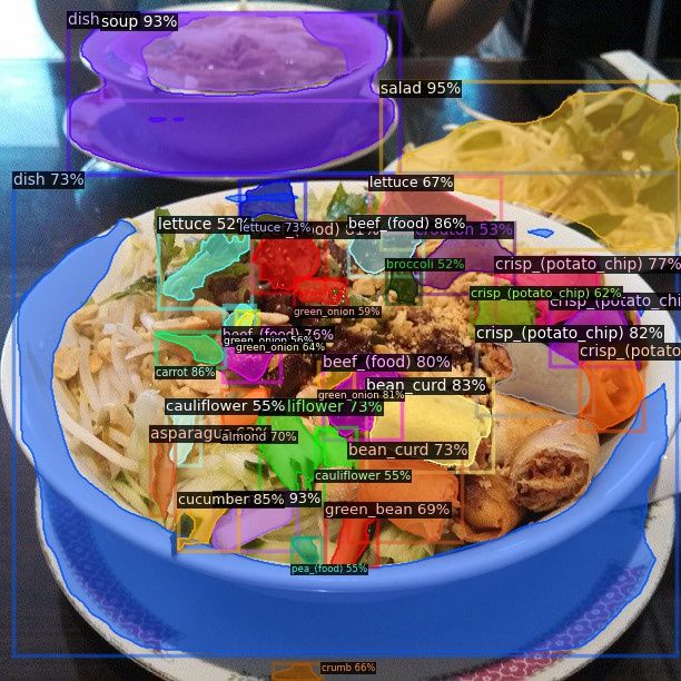
predictions, compared with only 30-40% of discouraging gra-        Resampling Methods. Oversampling methods (Chawla
 dients for frequent categories. Discouraging gradients from        et al. 2002; Han, Wang, and Mao 2005; Mahajan et al. 2018;
 background classification (orange curve) contribute a much         Hensman and Masko 2015; Huang et al. 2016; He et al.
 higher percentage of total discouraging gradients compared         2008; Zou et al. 2018) duplicate rare class samples to bal-
 to that of incorrect foreground prediction (blue curve) as used    ance out the class frequency distribution. However, over-
 in EQL (Tan et al. 2020). Figure 1(b) shows that using a           sampling methods tend to overfit to the rare categories, as
 ground-truth background anchor, a trained model predicts           this type of method does not address the fundamental lack
 scores for rare categories with several orders-of-magnitude        of data. Several oversampling methods aim to address this
 lower confidence than for frequent categories. This demon-         by augmenting the available data (Chawla et al. 2002; Han,
 strates a bias towards predicting more frequent categories.        Wang, and Mao 2005), but undersampling methods are often
    Based on these observations, we develop a simple yet effec-     preferred (Drummond, Holte et al. 2003). Undersampling
 tive method to adaptively rebalance the ratio of background        methods (Drummond, Holte et al. 2003; Tsai et al. 2019;
 prediction losses between rare/common and frequent cate-           Kahn and Marshall 1953) remove frequent class samples
 gories. Our proposed method DropLoss removes losses for            from the dataset to balance the class frequency distribution.
 rare and common categories from background predictions             The loss of information from removing these samples can
 based on sampling a Bernoulli variable with parameters de-         be mitigated through careful selection using statistical tech-
 termined by batch statistics. DropLoss prevents suppression        niques (Tsai et al. 2019; Kahn and Marshall 1953). It can
 of rare and common categories, increasing opportunities for        be beneficial to combine the advantages of undersampling
 correct predictions of infrequent classes during training and      and oversampling (Chawla et al. 2002). Dynamic methods
 reducing frequent class bias.                                      adjust the sampling distribution throughout training based on
    The contributions of this work are summarized as follows:       loss or metrics (Pouyanfar et al. 2018). Class balance sam-
1. We provide an analysis of the unique characteristics of          pling (Kang et al. 2019; Shen, Lin, and Huang 2016) uses
    long-tailed distributions, particularly in the context of in-   class-aware strategies to rebalance the data distribution for
    stance segmentation, to pinpoint the imbalance problem          learning classifiers and representations. In the context of the
    caused by disproportionate discouraging gradients from          dense instance segmentation problem, it is difficult to apply
    background predictions during training.                         the above resampling methods because the number of class
                                                                    examples per image may vary.
2. We develop a methodology for alleviating imbalances in
    the long-tailed setting by leveraging the ratio of rare and     Reweighting and Cost-sensitive Methods. Rather than re-
    frequent classes in a sampled training batch.                   balancing the sampling distribution, reweighting methods
3. We present state-of-the-art instance segmentation results        seek to balance the loss weighting between rare and frequent
    on the challenging long-tail LVIS dataset (Gupta, Dollár,      categories. Class frequency reweighing methods commonly
    and Girshick 2019).                                             use the inverse frequency of each class to weight the loss
                                                                    (Huang et al. 2016; Wang, Ramanan, and Hebert 2017; Cui
                       Related Work                                 et al. 2019). Cost-sensitive methods (Li, Liu, and Wang 2019;
                                                                    Lin et al. 2017d) aim to balance the model loss magnitudes be-
Object Detection and Instance Segmentation. Two-stage               tween rare and frequent categories. An existing meta-learning
detection architectures (Girshick et al. 2014; Girshick 2015;       method (Shu et al. 2019) explicitly learns loss weights based
Ren et al. 2015; Lin et al. 2017a) have been successful in          on the data. Our method provides a simple way to combine
the object detection setting, where the first stage proposes a      class frequency-aware sampling and cost-sensitive learning.
“region of interest” and the second stage refines the bounding
box and performs classification. This decomposition was             Feature Manipulation Methods. In contrast to resampling
initially proposed in R-CNN (Girshick et al. 2014). Fast R-         methods and reweighting methods that focus on modifying
CNN (Girshick 2015) and Faster R-CNN (Ren et al. 2015)              the loss based on class frequency, feature manipulation meth-
improve efficiency and quality for object detection. Mask R-        ods aim to design specific architectures or feature relation-
CNN later adapts Faster R-CNN to the instance segmentation          ships to address the long-tail problem. Normalization can be
setting by adding a mask prediction branch in the second            used to control the distribution of deep features, preventing
stage (He et al. 2017). Mask R-CNN has proven effective             frequent categories from dominating training (Kang et al.
in a wide variety of instance segmentation tasks. Our work          2019). Metric learning methods (Kang et al. 2019; Zhang
adopts this architecture. In contrast with two-stage methods,       et al. 2017) learn maximally-distant “prototypes” of deep
single-stage methods provide faster inference by eliminating        features to improve performance on data-scarce categories,
the region proposal stage and instead predicting a bounding         effectively transferring knowledge between head and tail cat-
box directly from anchors (Liu et al. 2016; Redmon et al.           egories. Similarly, knowledge transfer in feature space can
2016; Lin et al. 2017c). However, two-stage architectures           be accomplished using memory-based prototypes (Liu et al.
generally provide better localization.                              2019) or transfer of intra-class variance (Yin et al. 2019).
Learning Long-tailed Distributions. Techniques for learn-           Long-tail Learning Settings. Several methods have been
ing long-tailed distributions generally fall into three groups:     proposed to handle the problem of learning from imbalanced
resampling, reweighting and cost-sensitive learning, and fea-       datasets in other settings such as object classification (Cui
ture manipulation. We discuss each in the following sections.       et al. 2019; Cao et al. 2019; Jamal et al. 2020; Tan et al. 2020).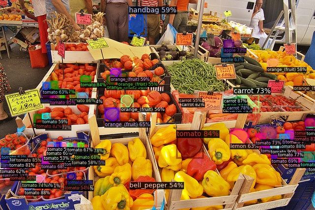
In the long-tail object recognition setting, the prior state-of-
the-art method (Tan et al. 2020) uses selective reweighting.
Their work observed that rare categories receive significantly
more “discouraging gradients” compared with frequent cate-
gories, and develop a method for rebalancing discouraging
gradients from foreground misclassifications. Their method
uses a binary 0 or 1 reweighting based on whether the class is
rare or frequent. Unlike this work, our method focuses on the
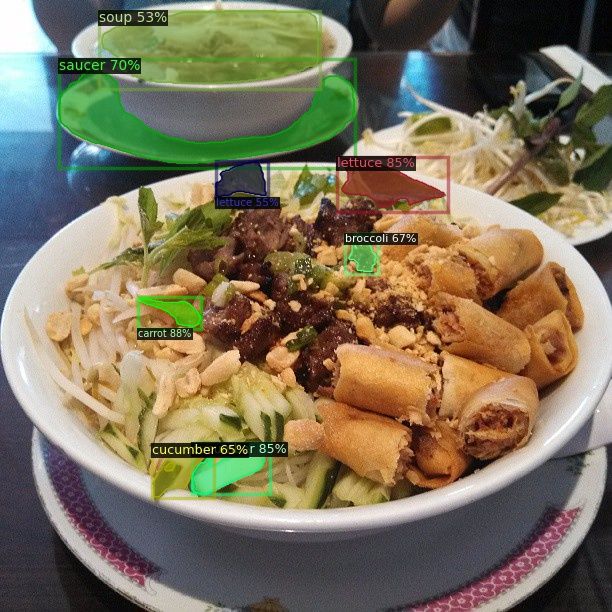
much more prevalent background classification losses in the (a) Weight wj as a function (b) Frequent-rare category
instance segmentation setting, and we develop a new adaptive of the logarithm base b. performance tradeoff
resampling and reweighting method which accounts for this
imbalance and for the distribution of classes within a sample. Figure 2: Background equalization loss. We present an ex-
Note that most of the methods for learning long-tailed distri- tension of the equalization loss that specifically focuses on
butions focus on the image classification setting where this is the background classification. (a) The curves of the LBEQL
no background class (and therefore no losses associated with weights in (4) with different choices for the logarithm base
background). In object detection and instance segmentation, b. Smaller values of the logarithm base b reduce the effects
however, the background class plays a very dominant role in of background more. (b) The experimental result of applying
the loss. This inspires our design of a reweighting mechanism different logarithm bases shows a tradeoff between the mean
which specifically considers background class. average precision (mAP) of rare categories and the mAP of
frequent categories with respect to different logarithm base
settings. Note that the background equalization loss LBEQL
Method with a large base b reduces to the existing equalization loss
LEQL .
Based on the observation that rare and common categories
receive disproportionate discouraging gradients from back-
ground classifications (compared with frequent categories), lated as follows:
C
the goal of our method is to prevent rare categories from X pj , if yj = 1 ,
being overly suppressed by reducing the imbalance of dis- LEQL = − wj log(p̂j ) , p̂j =
1 − pj , otherwise,
couraging gradients. We are inspired by work in one-stage j=1
object detection (Li, Liu, and Wang 2019; Lin et al. 2017d), (1)
which encounters a similar problem of large gradients from wj = 1 − E(r)Tλ (fj )(1 − yj ) , (2)
negative anchors inhibiting learning. We first construct a base- where C is the number of categories, pj is predicted logit,
line which modifies the equalization loss (Tan et al. 2020) and fj is the frequency of category j in the dataset. The in-
to rebalance gradients from foreground and background re- dicator function E(r) outputs 1 if r is a foreground region
gion proposals for rare/common and frequent categories. We and 0 if it belongs to the background. More specifically, for
show that this baseline leads to improved results over (Tan a region proposal r that is considered a background region
et al. 2020) but requires careful hyperparameter selection and with all yj being zero, we have E(r) = 0. Tλ (f ) is also
exhibits a clear tradeoff between rare/common and frequent a binary indicator function that, given a threshold λ, out-
categories. To alleviate this problem, we propose a stochastic puts 1 if f < λ to indicate the category is of low frequency.
DropLoss which improves the overall frequent-rare category It can be verified from (2) that, for a foreground region r
performance as well as improving the tradeoff as measured (i.e., E(r) = 1), the weight wj is either 1 or 1 − Tλ (fj ),
by a Pareto frontier 3. depending on the frequency of the ground-truth category j.
Further, if a category j is of low frequency (rare category), the
weight wj = 1 − Tλ (fj ) becomes zero and thus no penalty
Revisiting the Equalization Loss is given to incorrect foreground predictions. On the other
hand, for frequent categories, the weight is 1 and the penalty
Equalization Loss. We start with a review of the equaliza- of incorrect prediction remains − log(1 − pj ). By removing
tion loss (Tan et al. 2020). Equalization loss modifies sig- discouraging gradients to rare/common categories from in-
moid cross-entropy to alleviate discouraging gradients from correct foreground predictions, the equalization loss achieved
incorrect foreground predictions. Note that, in sigmoid cross- state-of-the-art on the LVIS Challenge 2019. Foreground
entropy, the ground-truth label yj represents only a binary class label prediction is selected using the maximum logit,
distribution for the foreground category j, and no extra class so entirely removing the loss allows the network to optimize
label for the background is included. That is, we have yj = 1 rare categories without penalties, as long as the prediction
if the ground-truth category of a region is j. On the other logit is less than ground truth for the frequent categories. This
hand, if a region belongs to the background, we have yj = 0 approach removes large penalties for non-zero confidences
for all the categories. During training, a region proposal is in rare categories, which otherwise imbalance the training to
labeled as “background” if its IoU with any ground-truth suppress rare categories.
region of a foreground class is lower than 50%. Background Equalization Loss. In contrast to the mech-
Given a region proposal r, the equalization loss is formu- anism of equalization loss that prevents large penalties for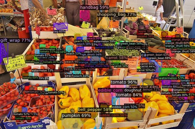
non-zero confidences in rare categories, cost-sensitive learn-    Bernoulli distribution by a beta sampling distribution over the
ing methods only reduce (Lin et al. 2017d) or remove (Li,         occurrence ratios of rare, common, and frequent categories
Liu, and Wang 2019) discouraging gradients if the magni-          for the regions generated by the Region Proposal Network
tude of the loss falls below some threshold. Our core insight     (Ren et al. 2015) during training. The Bernoulli distribution
is that foreground and background categories require differ-      with a Beta prior is suitable because we aim to model binary
ent approaches due to the differences in prediction criteria.     outcomes with varying biases in a stochastic manner.
For background categories, the network predicts background           Given a batch of region proposals, we compute the ratio
class if all logits pj fall below a threshold. For foreground     between the occurrences of ‘rare + common’ categories to
categories, the prediction is selected using the maximum logit    all foreground occurrences (i.e., ‘rare + common + frequent’
pj . Inspire by cost-sensitive loss and equalization loss, we     categories). In other words, we treat a batch of region propos-
present the background equalization loss as an extension to       als as a sample of occurrence ratio that is drawn from a beta
the original equalization loss:                                   distribution to provide the parameter of the Bernoulli distribu-
                                                                  tion. Our intuition behind such a scheme is simple: For region
                C
               X                           pj ,     if yj = 1 ,   proposals of rare and common categories, their occurrences
 LBEQL = −          wj log(p̂j ) , p̂j =                          in a batch are of low frequency. Therefore, the discouraging
                                           1 − pj , otherwise,
              j=1
                                                                  gradients from the background predictions should be accord-
                                                          (3)    ingly discounted for rare and common categories.
           1 − Tλ (fj )(1 − yj ),               if E(r) = 1 ,        We formulate DropLoss as follows:
 wj =
           1 − Tλ (fj ) · min{− logb (pj ), 1}, otherwise.                        C
                                                           (4)
                                                                                 X                          pj ,     if yj = 1 ,
                                                                    LDrop = −        wj log(p̂j ) , p̂j =
By comparing (2) and (4), we can see that the background                                                    1 − pj , otherwise,
                                                                                j=1
equalization loss differs from the equalization loss in the                                                                (5)
weights for background regions. The equalization loss al-
                                                                                   1 − Tλ (fj )(1 − yj ), if E(r) = 1 ,
ways penalizes a background region (E(r) = 0 and thus                     wj =                                             (6)
wj = 1) even if the category is of low frequency. In contrast,                     w ∼ Ber(µfj ),         otherwise,
our background equalization loss gives smaller weight to          where a random sample w ∈ {0, 1} is drawn from Bernoulli
background predictions as long as their confidences are low.      distribution Ber(µfj ) if the region proposal r belongs to
We use a logarithm base b to control the sensitivity of the       the background, i.e., E(r) = 0. The parameter µfj of the
weight concerning the confidence of background prediction.        Bernoulli distribution is determined by the occurrence ratio
Figure 2(a) shows the curves of the LBEQL weights in (4) by       of low-frequency (‘rare + common’) categories in the current
varying the value of the logarithm base b. For example, sup-      batch of region proposals. We compute the parameter by
pose we would want to focus on the performance of the rare
                                                                               (nrare + ncommon )/nall , if Tλ (fj ) = 1 ,
category, we can set the value of b = 2. The main idea here          µfj =                                                 (7)
is to alleviate the accumulation of small but non-negligible                   nfrequent /nall ,          otherwise,
discouraging gradients from the background. When applying         where nrare , ncommon , and nfrequent are the numbers of oc-
the proposed background equalization loss with different log-     currences of rare, common, and frequent categories in the
arithm bases, however, we see a clear performance tradeoff        current training batch of foreground region proposals. The
between frequent and rare categories (see Figure 2(b)). The       total number of foreground occurrences is nall = nrare +
results show that the average precision of the rare categories    ncommon + nfrequent . Implementation of the above DropLoss
behaves in the opposite way as the average precision of the       scheme is straightforward: For each batch, we derive the pa-
frequent categories for different choices of logarithm bases.     rameter µfj depending on whether category j is rare/common
                                                                  or frequent. We can then simulate a flip of a biased coin with
DropLoss                                                          head probability µfj and assign wj = 1 if we get a head.
While suppressing discouraging gradients from the back-              A region proposal is annotated as a background region if it
ground shows improvement for the rare categories, the back-       does not overlap with any ground-truth foreground region, or
ground equalization loss has a drawback. The performance          if the IoU is lower than 50%. If the number of rare category
often sensitively depends on the choice of the logarithm base.    occurrences in a given batch is large, discouraging gradients
It is difficult to choose an appropriate logarithm base that      to that rare category are more likely to be kept (with a higher
works for different long-tailed distributions without suffering   chance to get wj = 1). On the other hand, if a rare category
from a tradeoff between frequent and rare categories. In light    does not appear very often in a batch, it is highly probable that
of this, we propose a new stochastic method, called DropLoss,     discouraging gradients to the rare category will be dropped.
which dynamically balances the influence of background dis-       Therefore, our dropping strategy tends to neglect unrelated
couraging gradients for rare/common/frequent categories.          non-overlapping background proposals but would be inclined
   Similar to the design of the background equalization loss,     to keep more related (0 < IoU < 0.5) background proposals.
we seek to adjust weights on the logits of low-frequency
categories for background region proposals. In DropLoss, we                          Experimental Results
introduce a Bernoulli distribution and sample a binary value      In this section, we present the implementation details and
from the distribution as the weight wj if a region belongs to     experimental results. We compare DropLoss with the state-
the background. Further, we determine the parameter of the        of-the-art long-tail instance segmentation baselines on the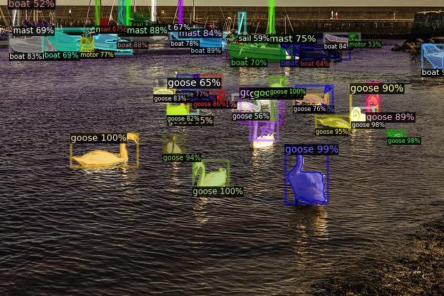
Architecture         Backbone        Loss                         AP (%)   AP50    AP75     APr     APc    APf     AR      APbbox
                                      BCE                           21.5    33.4     22.9    4.7     21.2   28.6    28.3      21
 Mask R-CNN           R-50-FPN        EQL (Tan et al. 2020)         23.8    36.3     25.2    8.5     25.2   28.3    31.5     23.5
                                      DropLoss (Ours)               25.5    38.7     27.2    13.2    27.9   27.3    34.8     25.1
                                      BCE                           23.6    36.5     25.1    5.6     24.2   30.1    30.9     23.3
 Mask R-CNN           R-101-FPN       EQL (Tan et al. 2020)         26.2    39.5     27.9    11.9    27.8   29.8    33.8     26.2
                                      DropLoss (Ours)               26.9    40.6     28.9    14.8    29.7   28.3    36.4     26.8
                                      BCE                           21.4     32      23.1    3.4     20.4   29.8    27.6     22.8
 Cascade R-CNN        R-50-FPN        EQL (Tan et al. 2020)         24.2    35.9     25.8    7.8      25    29.7    31.4      26
                                      DropLoss (Ours)                25      37      26.9    9.1     27.2   28.7     34      26.9
                                      BCE                            23     34.4     24.7    3.5     22.8   31.2    29.9     24.9
 Cascade R-CNN        R-101-FPN       EQL (Tan et al. 2020)         25.4    37.3     27.3    7.2     26.6    31     33.1     27.2
                                      DropLoss (Ours)               26.4     39      28.1    11.5    28.5   29.7    35.5     28.6

Table 1: Comparison between architecture and backbone settings, evaluated on LVIS v0.5 validation set. We compare BCE
(binary cross-entropy), EQL (equalization loss) and Drop (DropLoss). AP/AR refers to mask AP/AR, and subscripts ‘r’, ‘c’, and
‘f’ refer to rare, common, and frequent categories.

                                                                       We train the network using stochastic gradient descent with
                                                                       a momentum of 0.9 and a weight decay of 0.0001 for 90K
                                                                       iterations, with batch size 16 on eight parallel NVIDIA 2080
                                                                       Ti GPUs. We initialize the learning rate to 0.2 and decay it
                                                                       by a ratio of 0.1 at iterations 60,000 and 80,000. We use the
                                                                       Detectron2 (Wu et al. 2019) framework with default data
                                                                       augmentation. The data augmentation includes scale jitter
                                                                       with a short edge of (640, 672, 704, 736, 768, 800) pixels and
                                                                       a long edge no more than 1,333 pixels horizontal flipping. In
Figure 3: Measuring the performance tradeoff. Comparison               the Region Proposal Network (RPN), we sample 256 anchors
between rare, common, and frequent categories AP for base-             with a 1:1 ratio between foreground and background to com-
lines and our method. We visualize the tradeoff for ‘common            pute the RPN loss and choose 512 ROI-aligned proposals per
vs. frequent’ and ‘rare vs. frequent’as a Pareto frontier, where       image with a 1:3 foreground-background ratio for later pre-
the top-right position indicates an ideal tradeoff between ob-         dictions. Based on LVIS (Gupta, Dollár, and Girshick 2019),
jectives. DropLoss achieves an improved tradeoff between               the prediction threshold is reduced from 0.05 to 0.0, and we
object categories, resulting in higher overall AP.                     set the top 300 bounding boxes as prediction results. This
                                                                       setting is widely used in LVIS training and evaluation. For
                                                                       all the experiments, we report the average results of three
challenging LVIS dataset (Gupta, Dollár, and Girshick 2019).          independent runs of model training. The variances in AP are
To validate the effectiveness of this approach, we compare             generally small (approximately 0.1-0.2).
across different architectures and backbones and integrate
with additional long-tail resampling methods. We find that
DropLoss demonstrates consistently improved results in AP              Comparisons with state-of-the-art methods. In our ex-
and AR across all these experimental settings.                         periments, we use Mask R-CNN (He et al. 2017) as our
Dataset. Following the previous work equalization loss (Tan            architecture and compare it with two baseline training meth-
et al. 2020), we train and evaluate our model on LVIS bench-           ods: standard Mask R-CNN and the equalization loss (Tan
mark dataset. LVIS is a large vocabulary instance segmen-              et al. 2020). To verify that DropLoss is effective across dif-
tation dataset, containing 1,230 categories. In LVIS dataset,          ferent settings, we validate on several different architectures
categories are sorted into three groups based on the number            and backbones. We test ResNet50 and ResNet101 (He et al.
of images in which they appear: rare (1-10 images), common             2016) as backbones, and compare the Cascades R-CNN (Cai
(11-100), and frequent (> 100). We report AP for each bin to           and Vasconcelos 2018) as an alternative architecture to Mask
quantify performance in the long-tailed distribution setting.          R-CNN (He et al. 2020). Table 1 reports the results, where
We train our model on the 57K-image LVIS v0.5 training set             all methods are tested using the same experiment settings
and evaluate it on the 5K-image LVIS v0.5 validation set.              and environment. We find that DropLoss achieves improved
                                                                       performance (in terms of overall AP) compared with both
Implementation Details. For our experiments, we adopt                  baselines across all backbones and architectures. We are most
the Mask R-CNN (He et al. 2020) architecture with Feature              interested in the APr , APc , APf and AR. Although the APf
Pyramid Networks (Lin et al. 2017b) as a baseline model.               (frequent) decreases slightly in our method, our APr (rare)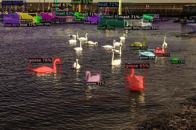
Method                        Use RFS       AP (%)      AP50         AP75      APr     APc      APf     APs      APm      APL      APbbox
    Sigmoid                           -           21.5       33.4        22.9      4.7     21.2     28.6    15.6     29.3      39        21
    Softmax                           -           21.3       33.1        22.6       3      21.2     28.6    15.8     28.5     39.2       21
    EQL (Tan et al. 2020)             -           23.8       36.3        25.2      8.5     25.2     28.3    17.1     31.4     41.7      23.5
    DropLoss (Ours)                   -           25.5       38.7        27.2      13.2    27.9     27.3    17.7     32.7     43.2      25.1
    Sigmoid                           X           23.8       36.3        25.2       8.5    25.2     28.3    17.1     31.4     41.7      23.5
    Softmax                           X           24.3       37.8        25.9      14.1    24.3     28.3    16.5     31.6     41.2      23.8
    EQL (Tan et al. 2020)             X           25.5        39         27.2      16.7    26.3     28.1    17.5      33       43        25
    DropLoss (Ours)                   X           26.4       40.3        28.4      17.3    28.7     27.2    17.9     33.1      44       25.8
    Method                        Use RFS       AP (%)      AP50         AP75      APr     APc      APf     APs      APm      APL      APbbox
    Baseline                          -           16.2       25.9        16.9      0.7     12.6      27     10.5     22.7     32.7      16.6
    EQL (Tan et al. 2020)             -           18.4       28.6        19.4      2.5     16.5     27.4    11.9     25.4     35.6      18.9
    DropLoss (Ours)                   -           19.8       30.9        20.9      3.5      20      26.7    12.9     27.5     37.1      20.4
    Baseline                          X           18.8       29.6        19.9       5.6    16.6     27.1    11.6     25.6     35.7      19.2
    EQL (Tan et al. 2020)             X            21        32.7        22.3       9.1    20.1     27.3    13.1     28.5     39.2      21.7
    DropLoss (Ours)                   X           22.3       34.5        23.6      12.4    22.3     26.5    13.9     29.9      40       22.9

Table 2: Evaluation on LVIS v0.5 (top) and LVIS v1.0 (bottom) validation sets with and without Repeat Factor Sampling (RFS).
Here we use Mask-RCNN and ResNet-50. DropLoss achieves the best overall AP across both settings.

and APc (common) increase significantly. Our method im-                         Tradeoff. Methods for learning long-tail distribution often
proves the AP and AR by a large margin, indicating the                          involve a tradeoff between accuracy on rare, common, and
overall performance across all categories is improved. In par-                  frequent categories. Here we wish to quantify this tradeoff
ticular, using Mask R-CNN with ResNet-50 as the backbone,                       for various methods. We compare our proposed DropLoss
we achieve a 1.7 AP improvement over the state-of-the-art                       against three baselines: equalization loss (Tan et al. 2020),
method (Tan et al. 2020) (winner of the LVIS 2019 chal-                         background equalization loss, and fixed drop ratio.
lenge). Across all the settings, compared with the baselines,                      Equalization loss and DropLoss have no tunable hyperpa-
DropLoss can more successfully balance the tradeoff between                     rameters. Background equalization loss has the log base as
rare and frequent categories, resulting in better performance                   a tunable hyperparameter. A fixed drop ratio has the drop
in the long-tailed distribution dataset.                                        ratio as a hyperparameter. These methods may be adjusted
Incorporating with Resampling Methods. Here we show                             to measure the tradeoff between object categories. We can
that our approach can be combined with state-of-the-art re-                     use the Pareto Frontier from multi-objective optimization to
sampling methods to improve learning long-tailed distribu-                      visualize this tradeoff, as seen in Figure 3. We observe that
tion further. Specifically, we adopt the Repeat Factor Sam-                     for reweighting methods with tunable hyperparameters, im-
pling (RFS) (Gupta, Dollár, and Girshick 2019) that uses the                   provement in rare APr or common APc generally leads to a
number of images per category to determine the sampling                         rapid decrease in frequent APf . Our proposed DropLoss does
frequency. Table 2 shows the quantitative comparisons of dif-                   not have tunable hyperparameters, but Figure 3 demonstrates
ferent loss function choices on the LVIS v0.5 validation set.1                  that DropLoss balances more effectively between APr , APc
We find that applying RFS generally improves the perfor-                        and APf , resulting in higher overall AP than other baselines.
mance of all the methods. The proposed DropLoss compares                           DropLoss adapts to the sampling distribution so that if a
favorably against other baseline methods either with or with-                   rare category appears in a given batch, its loss is less likely to
out using RFS. Note that the RFS method rebalances based                        be dropped. However, if a rare category does not appear in a
on overall data distribution, while DropLoss reweights the                      batch, the chance of its loss being dropped is very high. This
loss based on statistics in the each batch. The complementary                   allows the network to dynamically attend to the categories
nature of the two methods may explain why integrating RFS                       that it sees in a given batch, decreasing drop loss probability
and the DropLoss leads to improved results.                                     selectively for only those categories. We postulate that this al-
                                                                                lows the network to achieve a better overall balance between
Measuring the Frequent-rare Category Performance
                                                                                frequent and infrequent categories.
1
    Note that the EQL results (25.5 AP) are not consistent with the
    reported results (26.1 AP). We use the public implementation with-          Quantitative Comparison Between the DropLoss and
    out changes and report the average over 3 runs. The difference may          Our Proposed Baseline BEQL. To validate that the
    be due to number of GPUs used for training, resulting in differ-            DropLoss provides better pareto-efficiency over BEQL, in
    ent batch normalization. For fair comparisons, we use the same              Table 3, we compare the DropLoss with two best-performing
    hardware and experimental setting to train all models.                      results (in term of overall AP) from BEQL. DropLoss still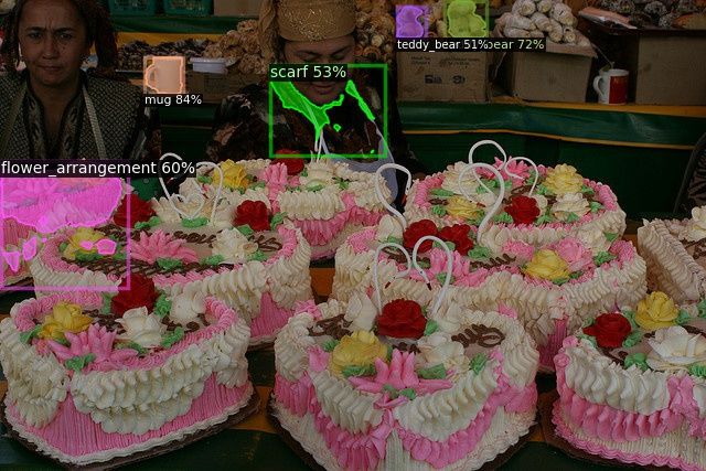
Mask RCNN with softmax loss

                                                  Mask RCNN with DropLoss

Figure 4: Visual results comparison. Qualitative results of the Mask R-CNN trained with standard cross-entropy loss (Top) and
the proposed DropLoss (Bottom). Instances with scores larger than 0.5 are shown.

offers overall better performance (not only in AP but also in    fication. By reducing the suppression of rare and common
AR) despite not sweeping the parameters on the validation        categories via background predictions, our method allows for
set to find the best performance as in BEQL.                     rare and common categories to improve prediction scores,
                                                                 decreasing bias towards frequent categories.

Method           AP (%) APr APc APf APbbox AR                                          Conclusions
                                                                 Through analysis of the loss gradient distributions over rare,
BEQL (b = 4) 25.2 14.6 28.1 25.9               24.9    34.1      common, and frequent categories, we discovered that dis-
BEQL (b = 5) 25.1 13.4 27.4 26.9               24.8    34.3      proportionate background gradients suppress less-frequent
DropLoss     25.5 13.2 27.9 27.3               25.1    34.8      categories in the long-tailed distribution problem. To ad-
                                                                 dress this problem, we propose DropLoss, which balances
                                                                 the background loss gradients between different categories
Table 3: Comparison between DropLoss and two top-                via random sampling and reweighting. Our method provides
performing results from our another proposed method BEQL.        a sizable performance improvement across different back-
Evaluation on LVIS v0.5 validation set. DropLoss offers over-    bones and architectures by improving the balance between
all better performance (in both AP and AR) compared with         object categories in the long-tail instance segmentation set-
the BEQL baseline.                                               ting. While we focus on the challenging problem of instance
                                                                 segmentation in our experiments, we expect that DropLoss
                                                                 may be applicable to other visual recognition problems with
Visual Results. Figure 4 demonstrates the results on a dense     long-tailed distributions. We leave the exploration to other
instance segmentation example containing common/rare cate-       tasks as future work.
gory. For example, the goose in the first image is a ‘common’
object category. We demonstrate the suppression of these less-                     Acknowledgments
frequent categories, as most of the geese in this image are
classified as background or with low confidence. In contrast,    This work was supported in part by Virginia Tech, the Min-
training the model with the proposed loss correctly identifies   istry of Education BioPro A+, and MOST Taiwan under
all geese as foreground, and predicts category “goose” with      Grant 109-2634-F-001-012. We are particularly grateful to
high confidence and other waterbirds with lower confidence.      the National Center for High-performance Computing for
Despite the stochastic removal of rare and common category       computing time and facilities.
losses for background proposals, we find that the network
does not misclassify background regions as foreground. The                              References
distinction between background and foreground is likely less     Cai, Z.; and Vasconcelos, N. 2018. Cascade R-CNN: Delving
difficult to learn than the distinction between foreground im-   into high quality object detection. In Proceedings of the IEEE
age categories, so reducing background gradients does not        conference on computer vision and pattern recognition, 6154–
appear to significantly affect background/foreground classi-     6162.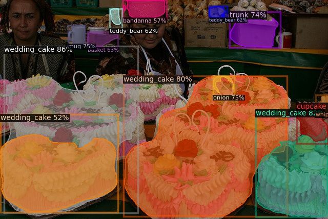
Cao, K.; Wei, C.; Gaidon, A.; Arechiga, N.; and Ma, T. 2019.      Kahn, H.; and Marshall, A. W. 1953. Methods of reducing
Learning imbalanced datasets with label-distribution-aware        sample size in Monte Carlo computations. Journal of the
margin loss. In Advances in Neural Information Processing         Operations Research Society of America 1(5): 263–278.
Systems.                                                          Kang, B.; Xie, S.; Rohrbach, M.; Yan, Z.; Gordo, A.; Feng,
Chawla, N. V.; Bowyer, K. W.; Hall, L. O.; and Kegelmeyer,        J.; and Kalantidis, Y. 2019. Decoupling representation
W. P. 2002. SMOTE: synthetic minority over-sampling tech-         and classifier for long-tailed recognition. arXiv preprint
nique. Journal of artificial intelligence research 16: 321–357.   arXiv:1910.09217 .
Cui, Y.; Jia, M.; Lin, T.-Y.; Song, Y.; and Belongie, S. 2019.    Li, B.; Liu, Y.; and Wang, X. 2019. Gradient harmonized
Class-balanced loss based on effective number of samples.         single-stage detector. In Proceedings of the AAAI Conference
In Proceedings of the IEEE Conference on Computer Vision          on Artificial Intelligence, volume 33, 8577–8584.
and Pattern Recognition, 9268–9277.
                                                                  Lin, T.-Y.; Dollár, P.; Girshick, R.; He, K.; Hariharan, B.; and
Drummond, C.; Holte, R. C.; et al. 2003. C4. 5, class imbal-      Belongie, S. 2017a. Feature pyramid networks for object de-
ance, and cost sensitivity: why under-sampling beats over-        tection. In Proceedings of the IEEE conference on computer
sampling. In Workshop on learning from imbalanced datasets        vision and pattern recognition, 2117–2125.
II, volume 11, 1–8. Citeseer.
                                                                  Lin, T.-Y.; Dollár, P.; Girshick, R.; He, K.; Hariharan, B.; and
Girshick, R. 2015. Fast R-CNN. In Proceedings of the IEEE         Belongie, S. 2017b. Feature pyramid networks for object de-
international conference on computer vision, 1440–1448.           tection. In Proceedings of the IEEE conference on computer
Girshick, R.; Donahue, J.; Darrell, T.; and Malik, J. 2014.       vision and pattern recognition, 2117–2125.
Rich feature hierarchies for accurate object detection and se-
                                                                  Lin, T.-Y.; Goyal, P.; Girshick, R.; He, K.; and Dollar, P.
mantic segmentation. In Proceedings of the IEEE conference
                                                                  2017c. Focal Loss for Dense Object Detection. In The IEEE
on computer vision and pattern recognition, 580–587.
                                                                  International Conference on Computer Vision (ICCV).
Gupta, A.; Dollár, P.; and Girshick, R. B. 2019. LVIS: A
Dataset for Large Vocabulary Instance Segmentation. In            Lin, T.-Y.; Goyal, P.; Girshick, R.; He, K.; and Dollár, P.
IEEE Conference on Computer Vision and Pattern Recogni-           2017d. Focal loss for dense object detection. In Proceedings
tion, CVPR 2019, Long Beach, CA, USA, June 16-20, 2019.           of the IEEE international conference on computer vision,
                                                                  2980–2988.
Han, H.; Wang, W.-Y.; and Mao, B.-H. 2005. Borderline-
SMOTE: a new over-sampling method in imbalanced data              Lin, T.-Y.; Maire, M.; Belongie, S.; Hays, J.; Perona, P.;
sets learning. In International conference on intelligent com-    Ramanan, D.; Dollár, P.; and Zitnick, C. L. 2014. Microsoft
puting, 878–887. Springer.                                        coco: Common objects in context. In European conference
                                                                  on computer vision, 740–755. Springer.
He, H.; Bai, Y.; Garcia, E. A.; and Li, S. 2008. ADASYN:
Adaptive synthetic sampling approach for imbalanced learn-        Liu, W.; Anguelov, D.; Erhan, D.; Szegedy, C.; Reed, S.; Fu,
ing. In 2008 IEEE international joint conference on neural        C.-Y.; and Berg, A. C. 2016. SSD: Single shot multibox
networks (IEEE world congress on computational intelli-           detector. In European conference on computer vision, 21–37.
gence), 1322–1328. IEEE.                                          Springer.
He, K.; Gkioxari, G.; Dollár, P.; and Girshick, R. 2017. Mask    Liu, Z.; Miao, Z.; Zhan, X.; Wang, J.; Gong, B.; and Yu, S. X.
R-CNN. In Proceedings of the IEEE international conference        2019. Large-scale long-tailed recognition in an open world.
on computer vision, 2961–2969.                                    In Proceedings of the IEEE Conference on Computer Vision
He, K.; Gkioxari, G.; Dollár, P.; and Girshick, R. B. 2020.      and Pattern Recognition, 2537–2546.
Mask R-CNN. IEEE Trans. Pattern Anal. Mach. Intell. .             Mahajan, D.; Girshick, R.; Ramanathan, V.; He, K.; Paluri,
He, K.; Zhang, X.; Ren, S.; and Sun, J. 2016. Identity map-       M.; Li, Y.; Bharambe, A.; and van der Maaten, L. 2018.
pings in deep residual networks. In European conference on        Exploring the limits of weakly supervised pretraining. In
computer vision, 630–645. Springer.                               Proceedings of the European Conference on Computer Vision
                                                                  (ECCV), 181–196.
Hensman, P.; and Masko, D. 2015. The impact of imbal-
anced training data for convolutional neural networks. De-        Pouyanfar, S.; Tao, Y.; Mohan, A.; Tian, H.; Kaseb, A. S.;
gree Project in Computer Science, KTH Royal Institute of          Gauen, K.; Dailey, R.; Aghajanzadeh, S.; Lu, Y.-H.; Chen,
Technology .                                                      S.-C.; et al. 2018. Dynamic sampling in convolutional neu-
                                                                  ral networks for imbalanced data classification. In 2018
Huang, C.; Li, Y.; Loy, C. C.; and Tang, X. 2016. Learn-
                                                                  IEEE conference on multimedia information processing and
ing Deep Representation for Imbalanced Classification. In
                                                                  retrieval (MIPR), 112–117. IEEE.
Proceedings of the IEEE conference on computer vision and
pattern recognition, 5375–5384.                                   Redmon, J.; Divvala, S.; Girshick, R.; and Farhadi, A. 2016.
Jamal, M. A.; Brown, M.; Yang, M.-H.; Wang, L.; and Gong,         You Only Look Once: Unified, real-time object detection. In
B. 2020. Rethinking Class-Balanced Methods for Long-              Proceedings of the IEEE conference on computer vision and
Tailed Visual Recognition from a Domain Adaptation Per-           pattern recognition, 779–788.
spective. In IEEE/CVF Conference on Computer Vision and           Ren, S.; He, K.; Girshick, R.; and Sun, J. 2015. Faster R-
Pattern Recognition.                                              CNN: Towards real-time object detection with region pro-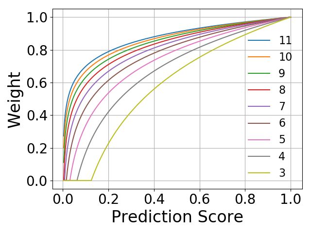
posal networks. In Advances in neural information process-
ing systems, 91–99.
Shen, L.; Lin, Z.; and Huang, Q. 2016. Relay backpropa-
gation for effective learning of deep convolutional neural
networks. In European conference on computer vision, 467–
482. Springer.
Shu, J.; Xie, Q.; Yi, L.; Zhao, Q.; Zhou, S.; Xu, Z.; and Meng,
D. 2019. Meta-weight-net: Learning an explicit mapping
for sample weighting. In Advances in Neural Information
Processing Systems, 1917–1928.
Tan, J.; Wang, C.; Li, B.; Li, Q.; Ouyang, W.; Yin, C.; and
Yan, J. 2020. Equalization Loss for Long-Tailed Object
Recognition. In Proceedings of the IEEE/CVF Conference
on Computer Vision and Pattern Recognition, 11662–11671.
Tsai, C.-F.; Lin, W.-C.; Hu, Y.-H.; and Yao, G.-T. 2019.
Under-sampling class imbalanced datasets by combining clus-
tering analysis and instance selection. Information Sciences
477: 47–54.
Wang, Y.-X.; Ramanan, D.; and Hebert, M. 2017. Learning to
model the tail. In Advances in Neural Information Processing
Systems, 7029–7039.
Wu, Y.; Kirillov, A.; Massa, F.; Lo, W.-Y.; and Girshick,
R. 2019. Detectron2. https://github.com/facebookresearch/
detectron2.
Yin, X.; Yu, X.; Sohn, K.; Liu, X.; and Chandraker, M. 2019.
Feature transfer learning for face recognition with under-
represented data. In Proceedings of the IEEE Conference on
Computer Vision and Pattern Recognition, 5704–5713.
Zhang, X.; Fang, Z.; Wen, Y.; Li, Z.; and Qiao, Y. 2017.
Range loss for deep face recognition with long-tailed training
data. In Proceedings of the IEEE International Conference
on Computer Vision, 5409–5418.
Zou, Y.; Yu, Z.; Vijaya Kumar, B.; and Wang, J. 2018. Un-
supervised domain adaptation for semantic segmentation via
class-balanced self-training. In Proceedings of the European
conference on computer vision (ECCV), 289–305.
You can also read