Scalable Feature Extraction with Aerial and Satellite Imagery
←
→
Page content transcription
If your browser does not render page correctly, please read the page content below
PROC. OF THE 17th PYTHON IN SCIENCE CONF. (SCIPY 2018)                                                                                                     145

   Scalable Feature Extraction with Aerial and Satellite
                        Imagery
                                                             Virginia Ng‡∗ , Daniel Hofmann‡

                                                     https://youtu.be/3AuRW9kq89g

                                                                                     F

Abstract—Deep learning techniques have greatly advanced the performance of
the already rapidly developing field of computer vision, which powers a variety
of emerging technologies—from facial recognition to augmented reality to self-
driving cars. The remote sensing and mapping communities are particularly
interested in extracting, understanding and mapping physical elements in the
landscape. These mappable physical elements are called features, and can
include both natural and synthetic objects of any scale, complexity and char-
acter. Points or polygons representing sidewalks, glaciers, playgrounds, entire
cities, and bicycles are all examples of features. In this paper we present a
method to develop deep learning tools and pipelines that generate features from
aerial and satellite imagery at large scale. Practical applications include object
detection, semantic segmentation and automatic mapping of general-interest
                                                                                                          Fig. 1: Computer Vision Pipeline.
features such as turn lane markings on roads, parking lots, roads, water, building
footprints.
     We give an overview of our data preparation process, in which data from             in the mappable landscape, we propose integrating deep neural
the Mapbox Satellite layer, a global imagery collection, is annotated with la-           network models into the mapping workflow. In particular, we have
bels created from OpenStreetMap data using minimal manual effort. We then
                                                                                         developed tools and pipelines to detect various geospatial features
discuss the implementation of various state-of-the-art detection and semantic
                                                                                         from satellite and aerial imagery at scale. We collaborate with
segmentation systems such as the improved version of You Only Look Once
(YOLOv2), modified U-Net, Pyramid Scene Parsing Network (PSPNet), as well
                                                                                         the OpenStreetMap [osm] (OSM) community to create reliable
as specific adaptations for the aerial and satellite imagery domain. We conclude         geospatial datasets, validated by trained and local mappers.
by discussing our ongoing efforts in improving our models and expanding their                Here we present two use cases to demonstrate our workflow
applicability across classes of features, geographical regions, and relatively           for extracting street navigation indicators such as turn restrictions
novel data sources such as street-level and drone imagery.                               signs, turn lane markings, and parking lots, in order to improve
                                                                                         our routing engines. Our processing pipelines and tools are de-
Index Terms—computer vision, deep learning, neural networks, satellite im-               signed with open source libraries including Scipy, Rasterio, Fiona,
agery, aerial imagery
                                                                                         Osium, JOSM, Keras, PyTorch, and OpenCV, while our training
                                                                                         data is compiled from OpenStreetMap and the Mapbox Maps API
I. Introduction                                                                          [mapbox_api]. Our tools are designed to be generalizable across
                                                                                         geospatial feature classes and across data sources.
Location data is built into the fabric of our daily experiences, and
is more important than ever with the introduction of new location-
based technologies such as self-driving cars. Mapping communi-
ties, open source or proprietary, work to find, understand and map                       II. Scalable Computer Vision Pipelines
elements of the physical landscape. However, mappable physical
                                                                                         The general design for our deep learning based computer vision
elements are continually appearing, changing, and disappearing.
                                                                                         pipelines can be found in Figure 1, and is applicable to both
For example, more than 1.2 million residential units were built in
                                                                                         object detection and semantic segmantation tasks. We design
the United States alone in 2017 [buildings]. Therefore, a major
                                                                                         such pipelines with two things in mind: they must scale to
challenge faced by mapping communities is maintaining recency
                                                                                         process petabytes worth of data; and they must be agile enough
while expanding worldwide coverage. To increase the speed and
                                                                                         to be repurposed for computer vision tasks on other geospatial
accuracy of mapping, allowing better pace-keeping with change
                                                                                         features. This requires tools and libraries that make up these
                                                                                         pipelines to be developed in modularized fashion. We present
* Corresponding author: virginia@mapbox.com
‡ Mapbox                                                                                 turn lane markings as an example of an object detection pipeline,
                                                                                         and parking lots as an example of a semantic segmentation
Copyright © 2018 Virginia Ng et al. This is an open-access article distributed           pipeline. Code for Robosat [robosat], our end-to-end semantic
under the terms of the Creative Commons Attribution License, which permits
unrestricted use, distribution, and reproduction in any medium, provided the             segmantion pipeline, along with all its tools, is made available
original author and source are credited.                                                 at: https://github.com/mapbox/robosat.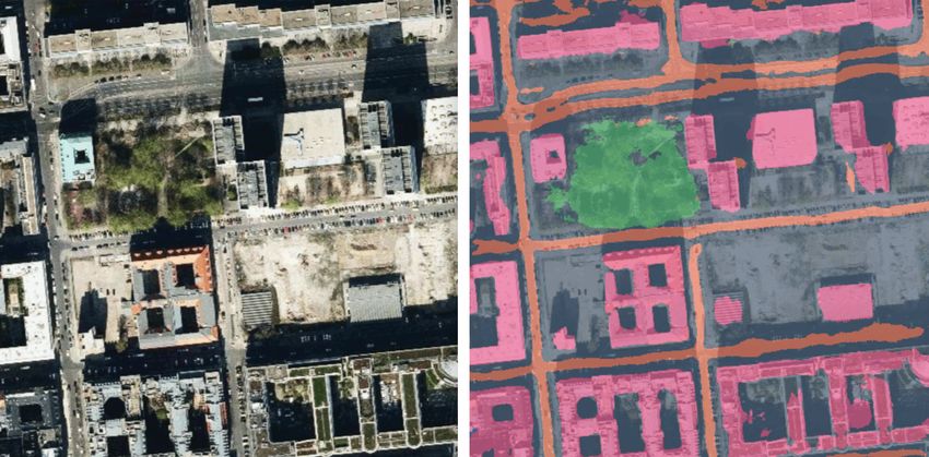
146 PROC. OF THE 17th PYTHON IN SCIENCE CONF. (SCIPY 2018)
Fig. 2: Left: Original satellite image. Right: Turn lane markings
detection.
1. Data
The data needed to create training sets depends on the type of
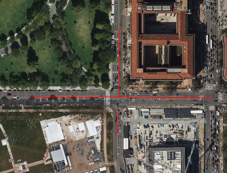
task: object detection or semantic segmentation. We first present Fig. 3: A custom layer created by clipping the locations of roads
our data preparation process for object detection and then discuss with turn lane markings to Mapbox Satellite. Streets with turn lane
the data preperation process for semantic segmentation. markings are rendered in red.
Data Preparation For Object Detection. Object detection is
the computer vision task that deals with locating and classifying a
variable number of objects in an image. Figure 2 demonstrates how
object detection models are used to classify and locate turn lane
markings from satellite imagery. There are many other practical
applications of object detection such as face detection, counting,
and visual search engines. In our case, detected turn lane markings
become valuable navigation assets to our routing engines when
determining the most optimal routes.
The turn lane marking training set is created by collecting im-
agery of various types of turn lane markings and manually drawing
a bounding box around each marking. We use Overpass Turbo1 to
query the OpenStreetMap database for streets containing turn lane
markings, i.e., those tagged with one of the following attributes:
“turn:lane=*”, “turn:lane:forward=*”, “turn:lane:backward=*” in
OpenStreetMap. The marked street segments, as shown in Figure
3, are stored as GeoJSON features clipped into the tiling scheme
[tile] of the Mapbox Satellite basemap [mapbox]. Figure 4 shows
how skilled mappers use this map layer as a cue to manually draw
bounding boxes around each turn lane marking using JOSM2 , a
process called annotation. These bounding boxes are stored in
GeoJSON polygon format on Amazon S3 [s3] and used as labels
during training.
Mappers annotate over 54,000 turn lane markings, span-
ning six classes - “Left”, “Right”, “Through”, “ThroughLeft”, Fig. 4: Annotating turn lane markings by drawing bounding boxes.
“ThroughRight”, and “Other” in five cities. Turn lane markings
of all shapes and sizes, as well as ones that are partially covered
by cars and/or shadows are included in this training set. To ensure
a high-quality training set, we had a separate group of mappers
verify each of the bounding boxes drawn. We exclude turn lane
markings that are not visible, as seen in Figure 5.
Data Engineering Pipeline for Object Detection. Within the
larger object detection pipeline, sits a data engineering pipeline
1. JOSM [josm] is an extensible OpenStreetMap editor for Java 8+. At its
core, it is an interface for editing OSM, i.e., manipulating the nodes, ways,
relations, and tags that compose the OSM database. Compared to other OSM
editors, JOSM is notable for its range of features, such as allowing the user
to load arbitrary GPX tracks, background imagery, and OpenStreetMap data
from local and online sources. It is open source and licensed under GPL. Fig. 5: Left: Examples of visible turn lane markings that are included
2. Overpass Turbo [overpass] is a web based data mining tool for Open- in the training set. Right: Defaced or obscured turn lane markings,
StreetMap. It runs any kind of Overpass API query and shows the results on such as those covered by cars, are excluded from the training set.
an interactive map.
SCALABLE FEATURE EXTRACTION WITH AERIAL AND SATELLITE IMAGERY 147
tract tool [rs-extract] in Robosat, our segmentation pipeline. These
parking lot polygons are stored as two-dimensional single-channel
numpy arrays, or binary mask clipped and scaled to the Mapbox
Satellite tiling scheme using the rs rasterize tool [rs-rasterize].
Each mask array is paired with its corresponding photographic
image tile. Conceptually, this can be compared to concatenating
a fourth channel, the mask, onto a standard red, green, and blue
image. 55,710 parking lots are annotated for the initial training set.
Fig. 6: Object Detection Data Engineering Pipeline: Annotated Open- Our tools and processes can be generalized to any OpenStreetMap
StreetMap GeoJSON features are converted to image pixel space, feature and any data source. For example, we also experiment with
stored as JSON image attributes and used as training labels. These
labels are then combined with each of their respective imagery tiles, building segmentation in unmanned aerial vehicle (UAV) imagery
fetched from the Mapbox Maps API (Satellite), to create a training set from the OpenAerialMap project in Tanzania [tanzania]. One can
for turn lane marking detection. generate training sets for any OpenStreetMap feature in this way
by writing custom Osmium handlers to convert OpenStreetMap
geometries into polygons.
2. Model
Fully Convolutional Neural Networks. Fully convolutional net-
works (FCNs) are neural networks composed only of convolu-
tional layers. They are contrasted with more conventional net-
works that typically have fully connected layers or other non-
convolutional subarchitectures as “decision-makers” just before
the output. For the purposes considered here, FCNs show several
significant advantages. First, FCNs can handle input images of
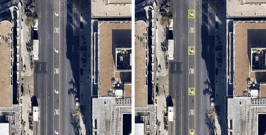
Fig. 7: Left: Original satellite image. Right: Semantic segmentation different resolutions, while most alternatives require input dimen-
of roads, buildings and vegetation. sions to be of a certain size [FCN]. For example, architectures
like AlexNet can only work with input images sizes that are 224
x 224 x 3 [FCN]. Second, FCNs are well suited to handling
designed to create and process training data in large quantities. spatially dense prediction tasks like segmentation because one
This data engineering pipeline is capable of streaming any set of would no longer be constrained by the number of object categories
prefixes off of Amazon S3 into prepared training sets. Several pre- or complexity of the scenes. Networks with fully connect layers, in
processing steps are taken to convert annotations to the appropriate contrast, generally lose spatial information in these layers because
data storage format before combining them with real imagery. The all output neurons are connected to all input neurons [FCN].
turn lane marking annotations are initially stored as GeoJSON Object Detection Models. Many of our applications require
polygons grouped by class. Each of these polygons is streamed out low latency prediction from their object detection algorithms.
of the GeoJSON files on S3, converted to image pixel coordinates, We implement YOLOv2 [yolov2], the improved version of the
and stored as JSON image attributes to abstract tiles [tile]. The real-time object detection system You Only Look Once (YOLO)
pre-processed annotations are randomly assigned to training and [yolo], in our turn lane markings detection pipeline. YOLOv2
testing datasets with a ratio of 4:1. The abstract tiles are then outperforms other state-of-the-art methods, like Faster R-CNN
replaced by the corresponding real image tiles, fetched from the with ResNet [resnet] and Single Shot MultiBox Detector (SSD)
Satellite layer of the Mapbox Maps API. At this point, each [ssd], in both speed and detection accuracy [yolov2]. It works
training sample consisted of a photographic image paired with its by first dividing the input image into 13 × 13 grid cells (i.e.,
corresponding JSON image attribute. Finally, the training and test there are 169 total cells for any input image). Each grid cell is
sets are zipped and uploaded to Amazon S3. This process is scaled responsible for generating 5 bounding boxes. Each bounding box
up to run multiple cities in parallel on Amazon Elastic Container is composed of its center coordinates relative to the location of its
Service3 . This data engineering pipeline is shown in Figure 6. corresponding grid cell, its normalized width and height, a confi-
Data Preparation for Semantic Segmentation. Semantic dence score for "objectness," and an array of class probabilities.
segmentation is the computer vision task that partitions an image A logistic activation is used to constrain the network’s location
into semantically meaningful parts, and classifies each part into prediction to fall between 0 and 1, so that the network is more
one of any pre-determined classes. This can be understood as stable. The objectness predicts the intersection over union (IOU)
assigning a class to each pixel in the image, or equivalently of the ground truth and the proposed box. The class probabilities
as drawing non-overlapping masks or polygons with associated predict the conditional probability of each class for the proposed
classes over the image. As an example of the polygonal approach, object, given that there is an object in the box [yolov2].
in addition to distinguishing roads from buildings and vegetation, 6 classes are defined for the turn lane markings detection
we also delineate the boundaries of each object in Figure 7. project. With 4 coordinates defining each box’s geometry, the
The parking lot training set is created by combining imagery
tiles collected from Mapbox Satellite with parking lots poly- 3. Osmium [osmium] is a fast and flexible C++ library for working with
OpenStreetMap data.
gons. Parking lot polygons are generated by querying the Open-
4. Amazon ECS [ecs] is a highly scalable, fast, container management
StreetMap database with Osmium [osmium] for OpenStreetMap service that makes it easy to run, stop, and manage Docker containers on
features with attributes “tag:amenity=parking=*” using the rs ex- specified type of instances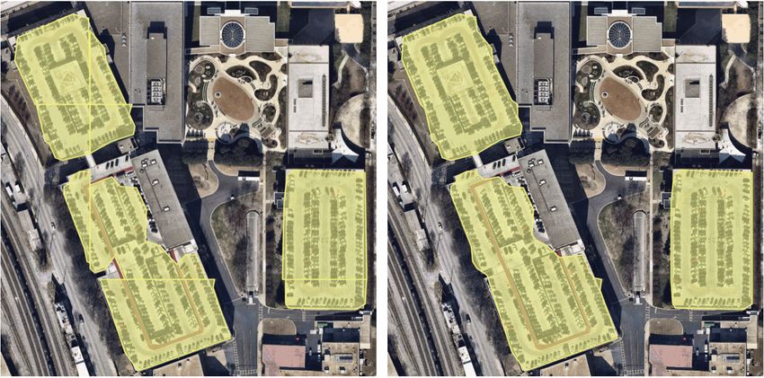
148 PROC. OF THE 17th PYTHON IN SCIENCE CONF. (SCIPY 2018)
Fig. 8: Clustering of box dimensions in the turn lane marking training
set. We run k-means clustering on the dimensions of bounding boxes
to get anchor boxes for our model. We used k = 5, as suggested by Fig. 9: U-Net architecture.
the YOLOv2 authors, who found that this cluster count gives a good
tradeoff for recall v. complexity of the model.
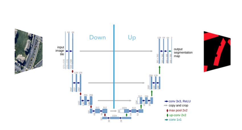
and can yield more precise segmentations than prior state-of-the-
art methods such as sliding-window convolutional networks. The
"objectness" confidence, and 6 class probabilities, each bounding first part of the U-Net network downsamples, and is similar in
box object is comprised of 11 numbers. Multiplying by boxes per design and purpose to the encoding part of an autoencoder. It
grid cell and grid cells per image, this project’s YOLOv2 network repeatedly applies convolution blocks followed by maxpool down-
therefore always yields 13 x 13 x 5 x 11 = 9,295 outputs per samplings, encoding the input image into increasingly abstract
image. representations at successively deeper levels. The second part of
The base feature extractor of YOLOv2 is Darknet-19 the network consists of upsampling and concatenation, followed
[darknet], a FCN composed of 19 convolutional layers and 5 by ordinary convolution operations. Concatenation combines rela-
maxpooling layers. Detection is done by replacing the last convo- tively “raw” information with relatively “processed” information.
lutional layer of Darknet-19 with three 3 × 3 convolutional layers, This can be understood as allowing the network to assign a class
each outputting 1024 channels. A final 1 × 1 convolutional layer to a pixel with sensitivity to small-scale, less-abstract information
is then applied to convert the 13 × 13 × 1024 output into 13 × about the pixel and its immediate neighborhood (e.g., whether it
13 × 55. We follow two suggestions proposed by the YOLOv2 is gray) and simultaneously with sensitivity to large-scale, more-
authors when designing our model. The first is incorporating abstract information about the pixel’s context (e.g., whether there
batch normalization after every convolutional layer. During batch are nearby cars aligned in the patterns typical of parking lots).
normalization, the output of a previous activation layer is nor- we gain a modest 1% improvement in accuracy by making two
malized by subtracting the batch mean and dividing by the batch additional changes. First we replace the standard U-Net encoder
standard deviation. This technique stabilizes training, improves with pre-trained ResNet50 [resnet] encoder. Then, we switch
the model convergence, and regularizes the model [yolov2_batch]. out the learned deconvolutions with nearest neighbor upsampling
By including batch normalization, YOLOv2 authors saw a 2% followed by a convolution for refinement.
improvement in mAP on the VOC2007 dataset [yolov2] compared We experiment with a Pyramid Scene Parsing Network (PSP-
to the original YOLO model. The second suggestion is the use Net) [pspnet] architecture for a 4-class segmentation task on
of anchor boxes and dimension clusters to predict the actual buildings, roads, water, and vegetation. PSPNet is one of the few
bounding box of the object. This step is acheieved by running pixel-wise segmentation methods that focuses on global priors,
k-means clustering on the turn lane marking training set bounding while most methods fuse low-level, high resolution features with
boxes. As seen in Figure 8, the ground truth bounding boxes for high-level, low resolution ones to develope comprehensive feature
turn lane markings follow specific height-width ratios. Instead of representations. Global priors can be especially useful for objects
directly predicting bounding box coordinates, our model predicts that have similar spatial features. For instance, runways and
the width and height of the box as offsets from cluster centroids. freeways have similar color and texture features, but they belong
The center coordinates of the box relative to the location of filter to different classes, which can be discriminated by adding car and
application is predicted by using a sigmoid function. building information. PSPNet uses pre-trained ResNet to generate
Our model is first pre-trained on ImageNet 224 × 224 res- a feature map that is 1/8 the size of the input image. The feature
olution imagery. The network is then resized and fine-tuned for map is then fed through the pyramid parsing module, a hierarchical
classification on 448 × 448 turn lane marking imagery, to ensure global prior that aggregates different scales of information. After
that the relatively small features of interest are still reliably upsampling and concatenation, the final feature representatation is
detected. fused with a 3 x 3 convolution to produce the final prediction map.
Segmentation Models. For parking lot segmentation, we As seen in Figure 6, PSPNet produced good-quality segmentation
select an approach of binary segmentation (distinguishing parking masks in our tests on scenes with complex features such as irreg-
lots from the background), and found U-Net [unet] to be a suitable ularly shaped trees, buildings and roads. For the 2-class parking
architecture. The U-Net architecture can be found in Figure 9. It lot task, however, we found PSPNet unnecessarily complex and
consists of a contracting path, to capture context, and a symmetric time-consuming.
expanding path, which allows precise localization. This type of Hard Negative Mining. This is a technique we apply to
network can be trained end-to-end with very few training images improve model accuracy [hnm] . We first train a model with an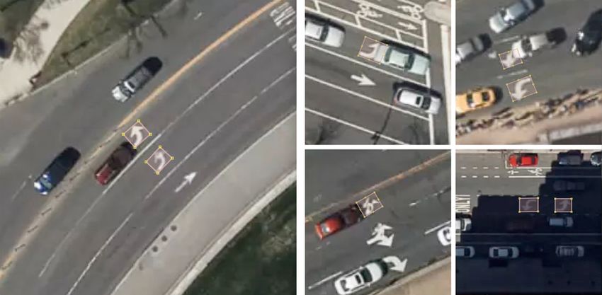
SCALABLE FEATURE EXTRACTION WITH AERIAL AND SATELLITE IMAGERY                                                                              149

Fig. 10: A probability mask marking the pixels that our model believes   Fig. 11: An example of border artifacts and holes in raw segmentation
belong to parking lots.                                                  masks produced by our U-Net model.

initial subset of negative examples, and collect negative examples
that are incorrectly classified by this initial model to form a set of
hard negatives. A new model is then trained with the hard negative
examples and the process may be repeated a few times.
     Figure 10 shows a model’s output as a probability mask
overlaid on Mapbox Satellite. Increasingly opaque red indicates
an increasingly high probability estimate of the underlying pixel
belonging to a parking lot. We use this type of visualization to find
representative falsely detected patches for use as hard negatives in
hard negative mining.
                                                                         Fig. 12: Left: Polygons crossing tile boundaries, and other adjacent
3. Post-Processing
                                                                         polygons, are combined. Right: Combined polygons.
Figure 11 shows an example of the raw segmentation mask derived
from our U-Net model. It cannot be used directly as input for
OpenStreetMap. We perform a series of post-processing steps to               Merging multiple polygons. This tool combines polygons
refine and transform the mask until it met quality and format            that are nearly overlapping, such as those that represent a single
requirements for OpenStreetMap consumption:                              feature broken by tile boundaries, into a single polygon. See
    Noise Removal. Noise in the output mask is removed by two            Figure 12.
morphological operations: erosion followed by dilation. Erosion              Deduplication. Cleaned GeoJSON polygons are compared
removes some positive speckle noise ("islands"), but it also shrinks     against parking lot polygons that already exist in OpenStreetMap,
objects. Dilation re-expands the objects.                                so that only previously unmapped features are uploaded.
    Fill in holes. The converse of the previous step, removing               All post-processing tools can be found in our Robosat
"lakes" (small false or topologically inconvenient negatives) in the     [robosat] GitHub repository.
mask.
    Contouring. During this step, continuous pixels having same
                                                                         4. Conclusion
color or intensity along the boundary of the mask are joined. The
output is a binary mask with contours.                                   We demonstrated the steps to building deep learning-based com-
    Simplification. We apply Douglas-Peucker simplification              puter vision pipelines that can run object detection and segmen-
[DP], which takes a curve composed of line segments and gives a          tation tasks at scale. With these pipeline designs, we are able
similar curve with fewer vertexes. OpenStreetMap favors polygons         to create training data with minimal manual effort, experiment
with the least number of vertexes necessary to represent the ground      with different network architectures, run inference, and apply post-
truth accurately, so this step is important to increase the data’s       process algorithms to tens of thousands of image tiles in parallel
quality as percieved by its end users.                                   using Amazon ECS. The outputs of the processing pipelines
    Transform Data. Polygons are converted from in-tile pixel            discussed are turn lane markings and parking lots in the form of
coordinates to GeoJSONs in geographic coordinates (longitude             GeoJSON features suitable for adding to OpenStreetMap. Mapbox
and latitude).                                                           routing engines then take these OpenStreetMap features into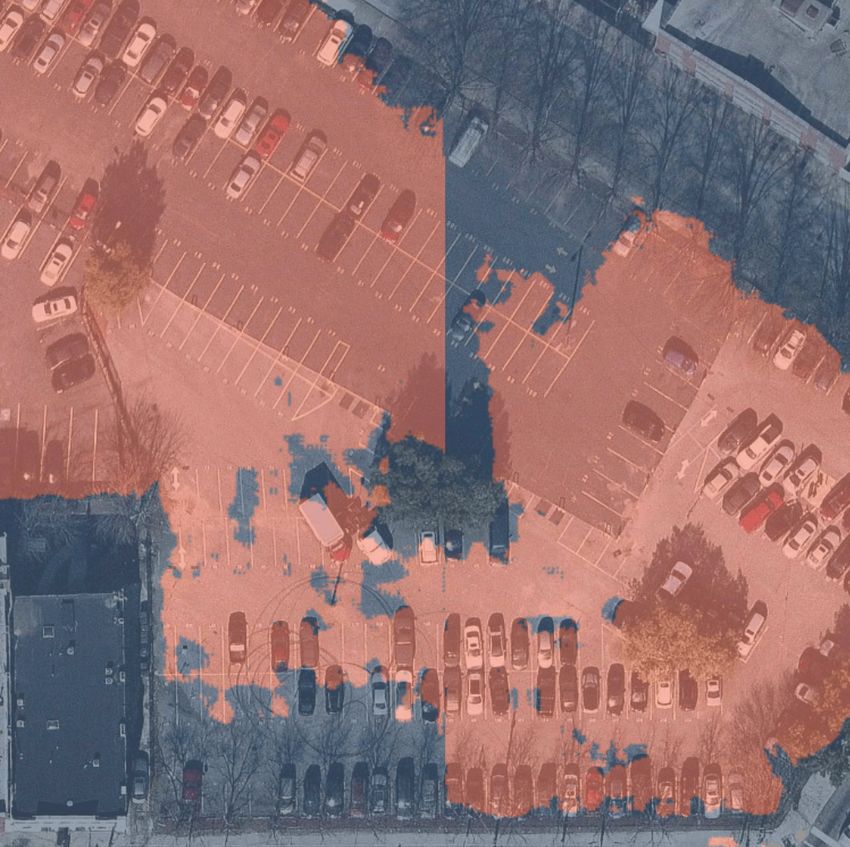
150                                                                                         PROC. OF THE 17th PYTHON IN SCIENCE CONF. (SCIPY 2018)

                                                                        the OpenStreetMap community [turn-restrict] in June 2018. For
                                                                        future work we will continue to look for ways to bring different
                                                                        sources and structures of data together to build better computer
                                                                        vision pipelines.

                                                                        R EFERENCES
                                                                        [buildings]    Cornish, C., Cooper, S., Jenkins, S., & US Census Bu-
                                                                                       reau. (2011, August 23). US Census Bureau New Resi-
                                                                                       dential Construction. Retrieved from https://www.census.gov/
                                                                                       construction/nrc/index.html
                                                                        [osm]          OpenStreetMap Contributors. (2017). OpenStreetMap. Re-
                                                                                       trieved May 30, 2018, from https://www.openstreetmap.org/
                                                                        [mapbox]       Mapbox. (n.d.). About. Retrieved June 30, 2018, from https:
                                                                                       //www.mapbox.com/about/
                                                                        [mapbox_api] Mapbox. (n.d.). Mapbox API Documentation. Retrieved May
Fig. 13: Front-end UI for instant turn lane marking detection on                       30, 2018, from https://www.mapbox.com/api-documentation/
Mapbox Satellite layer, a global imagery collection.                                   #maps
                                                                        [osm-lanes]    OpenStreetMap Contributors. (2018, February 27). Lanes.
                                                                                       Retrieved May 30, 2018, from https://wiki.openstreetmap.org/
                                                                                       wiki/Lanes
account when calculating optimal navigation routes. As we make          [overpass]     Raifer, M. (2017, January). Overpass Turbo. Retrieved from
various improvements to our baseline model and post-processing                         https://overpass-turbo.eu/
                                                                        [josm]         Scholz, I., & Stöcker, D. (2017, May). Java OpenStreetMap
algorithms (see below), we keep human control over the final                           Editor. Retrieved from https://josm.openstreetmap.de/
decision to add a given feature to OpenStreetMap. Figure 13             [osm-parking] OpenStreetMap Contributors. (2018, April). Tag:amenity=
shows a front-end user interface (UI) created to allow users to                        parking. Retrieved from https://wiki.openstreetmap.org/wiki/
                                                                                       Tag:amenity%3Dparking
run instant turn lane marking detection and visualize the results       [rs-extract]   Mapbox. (2018, June). Robosat. Retrieved from https://github.
on top of Mapbox Satellite. Users can select a model, adjust the                       com/mapbox/robosat#rs-extract
level of confidence for the model, choose from any Mapbox map           [rs-rasterize] Mapbox. (2018, June). Robosat. Retrieved from https://github.
styles [mapbox_style], and determine the area on the map to run                        com/mapbox/robosat#rs-rasterize
                                                                        [osmium]       Topf, J. (2018, April). Osmcode/libosmium. Retrieved May
inference on [mapbox_zoom].                                                            11, 2018, from https://github.com/osmcode/libosmium
                                                                        [tile]         OpenStreetMap Contributors. (2018, June). Tile Scheme.
                                                                                       Retrieved from https://wiki.openstreetmap.org/wiki/Slippy_
IV. Future Work                                                                        map_tilenames
                                                                        [tanzania]     Hofmann, D. (2018, July 5). Daniel-j-h’s diary | RoboSat
We are now working on making a few improvements to Robosat,                            loves Tanzania. Retrieved from https://www.openstreetmap.
our segmentation pipeline, so that it becomes more flexible in                         org/user/daniel-j-h/diary/44321
handling input image of different resolutions. First, our existing      [s3]           Amazon. (n.d.). Cloud Object Storage | Store & Retrieve Data
post-processing handler is designed for parking lot features and is                    Anywhere | Amazon Simple Storage Service. Retrieved from
                                                                                       https://aws.amazon.com/s3/
specifically tuned with thresholds set for zoom level 18 imagery        [ecs]          Amazon. (n.d.). Amazon ECS - run containerized applications
[osm_zoom]. We are replacing these hard-coded thresholds with                          in production. Retrieved from https://aws.amazon.com/ecs/
generalized ones that are calculated based on resolution in meters      [yolo]         Redmon, J., Divvala, S., Girshick, R., & Farhadi, A. (2016,
                                                                                       June). You Only Look Once: Unified, Real-Time Object
per pixel. We also plan to experiment with a feature pyramid-
                                                                                       Detection. 2016 IEEE Conference on Computer Vision and
based deep convolutional network called Feature Pyramid Net-                           Pattern Recognition (CVPR). doi:10.1109/cvpr.2016.91
work (FPN) [FPN]. It is a practical and accurate solution to            [ssd]          Liu, W., Anguelov, D., Erhan, D., Szegedy, C., Reed, S., Fu,
multi-scale object detection. Similar to U-Net, the FPN has lateral                    C., & Berg, A. C. (2016, September 17). SSD: Single Shot
                                                                                       MultiBox Detector. Computer Vision – ECCV 2016 Lecture
connections between the bottom-up pyramid (left) and the top-                          Notes in Computer Science, 21-37. doi:10.1007/978-3-319-
down pyramid (right). The main difference is where U-net only                          46448-0_2
copies features and appends them, FPN applies a 1x1 convolution         [darknet]      Redmon, J. (2013-2016). Darknet: Open Source Neural Net-
layer before adding the features. We will most likely follow the                       works in C. Retrieved from https://pjreddie.com/darknet/
                                                                        [yolov2]       Redmon, J., & Farhadi, A. (2017, July). YOLO9000: Better,
authors’ footsteps and use ResNet as the backbone of this network.                     Faster, Stronger. 2017 IEEE Conference on Computer Vision
    There two other modifications planned for the post-processing                      and Pattern Recognition (CVPR). doi:10.1109/cvpr.2017.690
steps. First, we want to experiment with a more sophisticated           [yolov2_batch] Ioffe, S., & Szegedy, C. (2015, February 11). Batch normaliza-
                                                                                       tion: Accelerating deep network training by reducing internal
polygon simplication algorithm besides Douglas-Peucker. Second,                        covariate shift.arXiv:1502.03167
we are rethinking the ordering of first performing simplication         [FCN]          Long, J., Shelhamer, E., & Darrell, T. (2015, June). Fully
then merging. The current post-process workflow performs simpli-                       Convolutional Networks for Semantic Segmentation. 2015
cation on individual extracted polygons and then merges polygons                       IEEE Conference on Computer Vision and Pattern Recogni-
                                                                                       tion (CVPR). doi:10.1109/CVPR.2015.7298965
that are across imagery tiles together. The resulting polygons,         [unet]         Ronneberger, O., Fischer, P., & Brox, T. (2015, May 18) U-
according to this process, may no longer be in the simplest shape.                     Net: Convolutional Networks for Biomedical Image Segmen-
    We design our tools and pipelines with the intent that other                       tation. 2015 MICCAI. arXiv:1505.04597
                                                                        [resnet]       He, K., Zhang, X., Ren, S., & Sun, J. (2016, June). Deep
practitioners would find it straightforward to adapt them to other                     Residual Learning for Image Recognition. 2016 IEEE Con-
landscapes, landscape features, and imagery data sources. For in-                      ference on Computer Vision and Pattern Recognition (CVPR).
stance, we generated 184,000 turn restriction detections following                     doi:10.1109/cvpr.2016.90
a similar process applying deep learning models on Microsoft’s          [pspnet]       Zhao, H., Shi, J., Qi, X., Wang, X., & Jia, J. (2017,
                                                                                       July). Pyramid Scene Parsing Network. 2017 IEEE Confer-
street-level imagery [streetside]. We released these turn restriction                  ence on Computer Vision and Pattern Recognition (CVPR).
detections located across 35,200 intersections and 23 cities for                       doi:10.1109/cvpr.2017.660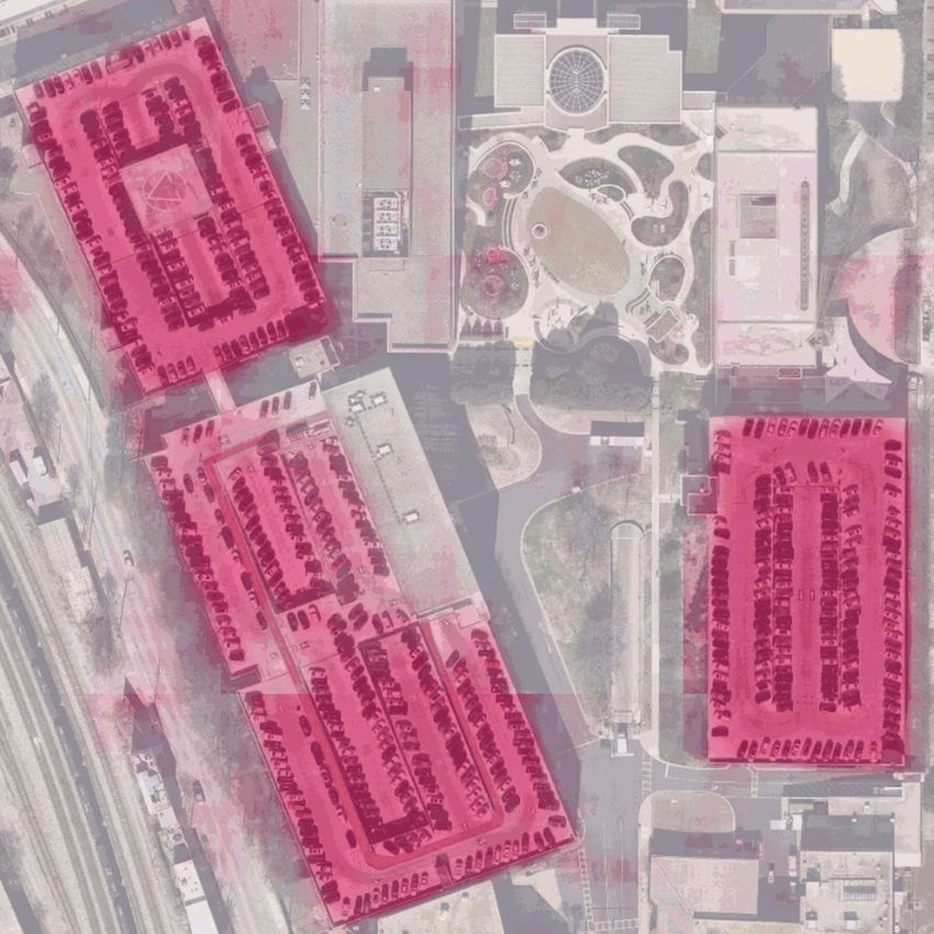
SCALABLE FEATURE EXTRACTION WITH AERIAL AND SATELLITE IMAGERY                   151

[hnm]           Dalal, N., & Triggs, B. (2005, June). Histograms of ori-
                ented gradients for human detection. 2005 IEEE Con-
                ference on Computer Vision and Pattern Recognition.
                10.1109/CVPR.2005.177
[robosat]       Mapbox. (2018, June). Robosat. Retrieved from https://github.
                com/mapbox/robosat
[DP]            Wu, S., & Marquez, M. (2003, October). A non-self-
                intersection Douglas-Peucker algorithm. 16th Brazilian Sym-
                posium on Computer Graphics and Image Processing (SIB-
                GRAPI 2003). doi:10.1109/sibgra.2003.1240992
[mapbox_style] Mapbox. (n.d.). Styles. Retrieved from https://www.mapbox.
                com/help/studio-manual-styles/
[mapbox_zoom] Mapbox. (n.d.). Zoom Level. Retrieved from https://www.
                mapbox.com/help/define-zoom-level/
[osm_zoom]      OpenStreetMap Contributors. (2018, June 20). Zoom Levels.
                Retrieved June 30, 2018, from https://wiki.openstreetmap.org/
                wiki/Zoom_levels
[FPN]           Lin, T., Dollar, P., Girshick, R., He, K., Hariharan, B., &
                Belongie, S. (2017, July). Feature Pyramid Networks for
                Object Detection. 2017 IEEE Conference on Computer Vision
                and Pattern Recognition (CVPR). doi:10.1109/cvpr.2017.106
[streetside]    Microsoft. (n.d.). Streetside. Retrieved from https://www.
                microsoft.com/en-us/maps/streetside
[turn-restrict] Ng, V. (2018, June 14). virginiayung’s diary | Releasing
                184K Turn Restriction Detections. Retrieved from https:
                //www.openstreetmap.org/user/virginiayung/diary/44171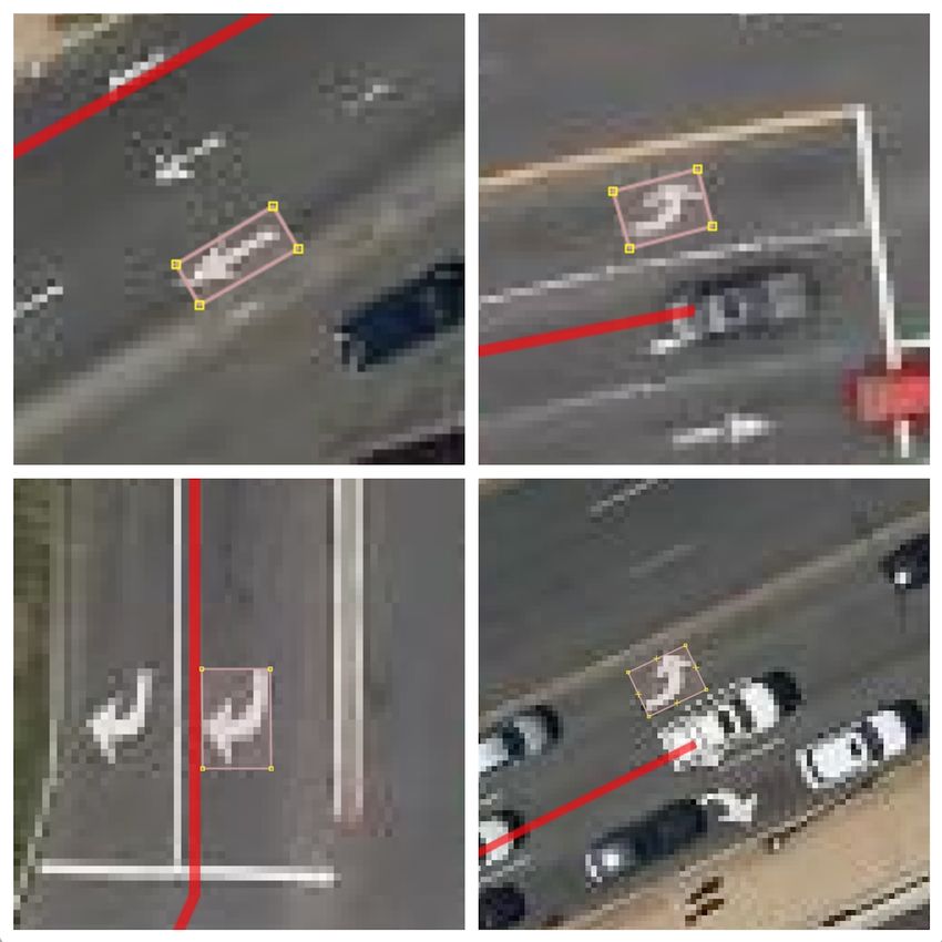
You can also read