URBAN CLASSIFICATION FROM AERIAL AND SATELLITE IMAGES - Sciendo
←
→
Page content transcription
If your browser does not render page correctly, please read the page content below
JOURNAL OF APPLIED ENGINEERING SCIENCES                                                                         VOL. 10(23), ISSUE 2/2020
ISSN: 2247-3769 / e-ISSN: 2284-7197                                                                              ART.NO. 299 pp. 163-172

    URBAN CLASSIFICATION FROM AERIAL AND SATELLITE IMAGES
                Iuliana Maria Pârvu a, b*, Iuliana Adriana Cuibac Picu a, b*, P.I. Dragomir c,
                                                Daniela Poli d
  a, b*
          National Center of Cartography, 012101 / Doctoral School, Technical University of Civil Engineering of Bucharest, 020396,
          Romania, e-mails: * iuliana.parvu@cngcft.ro / iuliana-maria.bina@phd.utcb.ro , iuliana.cuibac@cngcft.ro / iuliana-
                                                      adriana.cuibac@phd.utcb.ro
                             c
                               Faculty of Geodesy, Topography and Cadaster Department, Bucharest, Romania
                                    d
                                      Vermessung AVT-ZT-GmbH, Imst, Austria, e-mail: d.poli@avt.at

                     Received: 30.05.2020 / Accepted: 10.07.2020/ Revised: 06.10.2020 / Available online: 15.12.020

                                                 DOI: 10.2478/jaes-2020-0024

KEY WORDS: photogrammetry, multispectral images, support-vector machine, maximum likelihood classifier.

ABSTRACT:

When talking about land cover, we need to find a proper way to extract information from aerial or satellite images. In the field of
photogrammetry, aerial images are generally acquired by optical sensors that deliver images in four bands (red, green, blue and near-
infrared). Recent researches in this field demonstrated that for the image classification process is still place for improvement. From
satellites are obtained multispectral images with more bands (e.g. Landsat 7/8 has 36 spectral bands). This paper will present the
differences between these two types of images and the classification results using support-vector machine and maximum likelihood
classifier. For the aerial and the satellite images we used different sets of classification classes and the two methods mentioned above
to highlight the importance of choosing the classes and the classification method.

                       1. INTRODUCTION                                Hyperspectral images are acquired in pushbroom mode, do not
                                                                      have stereo coverage for 3D analysis, and are used for thematic
For urban and landscape analysis, photogrammetry and remote           information extraction, land classification, environmental
sensing allow to extract metric and thematic information of           studies, and so on. Moving to satellite platforms, Earth
objects directly from aerial or satellite images, without being in    observation satellites continuously acquire multi-spectral and
contact with the objects themselves. Images can be acquired at        hyperspectral imagery on any point of the Earth, with
different resolutions, in terms of geometry, spectrum,                differences similar to those mentioned in the aerial case.
radiometry, and time, depending on the platform, the type of
sensors and the application. In aerial photogrammetry large-          Multi-spectral optical sensor reach spatial resolution below 1
format multi-spectral cameras are used to acquire stereoscopic        metre and stereo coverage since the beginning of 2000’s for
images with four bands (RGBI – Red, Green, Blue and Near              photogrammetric processing and 2D/3D metric information
Infrared) for mapping applications (i.e. 2D / 3D cartography.         extraction at a scale of 1:10.000 and lower. On a spectral point
dense surface modelling, orthophoto production,). The scale of        of view, four bands are acquired in the visible and infrared
application is between scale 1:1.000 and 1:5.000, corresponding       domains and spectral information, with four additional spectral
to a ground sampling distance (GSD) of the images between 2           bands centered in the RedEdge, yellow, coastal, and near-
and 30 centimetres. Photogrammetric aerial flights are executed       infrared wavelengths, were introduced in 2015 with
at national scale on entire countries once every 2-3 years with       WorldView-2. The latest satellite of WorldView family, i.e.
the main purpose of generating true-colour or false-colour            WorldView-3, launched in 2014, has brought the spatial and
orthophotos, and update national spatial geodatabases. When           spectral resolution to extraordinary levels, by providing
combined with GIS (Geographic Information System) data, they          panchromatic images at a spatial resolution of 0.31 m, eight
are used for analysis, strategic planning and evaluation in urban     multispectral bands at 1.24 m, and eight additional Short Wave
planning and engineering. Hyperspectral cameras are also              InfraRed (SWIR) bands at a spatial resolution of 3.7 m
mounted on airplanes. They are medium-format cameras and              (DigitalGlobe, 2020). The images are available at a certain cost
images in larger spectral range with higher spectral resolution.      that depends on the area size, the age of the images, the order
For example, APEX camera (Vreys et al., 2016) acquires more           priority, the stereo availability and the type of licensing.
than 300 bands in VNIR (Visible and Near InfraRed) range (380         Hyperspectral satellite images are widely available with a long
– 870 nm) and about 200 bands in SWIR (Short Wave                     historical archive. Similar to the airborne case, hyperspectral
InfraRed) range (940 – 2500 nm), while HySpex (HySpex,                images do not have application in mapping, but in thematic
2020) acquires about 200 and 300 bands in VNIR and SWIR               information extraction, change detection and land cover
ranges respectively.                                                  classification.

* Corresponding authors: Iuliana Maria Pârvu / Iuliana Adriana Cuibac Picu - National Center of Cartography,
Cartography and Photogrammetry Department, 012101 / Doctoral School, Technical University of Civil Engineering of
Bucharest, 020396, Romania, e-mails: iuliana.parvu@cngcft.ro / iuliana.cuibac@cngcft.ro                                              163
JOURNAL OF APPLIED ENGINEERING SCIENCES                                                                       VOL. 10(23), ISSUE 2/2020
ISSN: 2247-3769 / e-ISSN: 2284-7197                                                                            ART.NO. 299 pp. 163-172

Indeed they have lower geometric resolution than multi-spectral
ones, due to a different acquisition principle and technology,
and acquire in a wider spectrum range with higher spectral
resolution. In most cases the missions are financed by national
space programs and images are available free of charge.

Satellite images are continuously acquired, with revisit time up
to few days, in case of constellations of satellites, thus
representing a fundamental source of information for change
detection in landscape monitoring, disaster damage assessment,
agricultural development and many other applications.

On the other hand aerial images are acquired on request;
therefore they provide a straightforward depiction of the
physical and cultural landscape of an area at a given time.
                                                                        Figure 1. First aerial image over Boston city (Boston as the
Aerial and satellite images are widely used for urban                              eagle and the wild goose see it, 2020)
classification, and the choice of the bands and the data depends
on the application and the data availability.                         In the time of analogue photogrammetry (1900-1960), it was
                                                                      discovered the first reliable black and white infrared sensor,
In this paper, we will focus on the classification of aerial images   which was used by the military sector. In the same period the
and satellite images on an urban environment, in order to             color film was developed, which contains three emulsion layers
evaluate the potential of each data and their applicability. As       sensitive to blue, green, and red. The computers were developed
working environment, the software ENVI 5.3 (developed by              in the analytical photogrammetry period (1960-2000), and then
Harris Corporation) was used. In Section 2 we will briefly            the specialists converted the analogue images into digital
report some historical notions about the development of aerial        images (made of pixels), by scanning process (Wolf et al.,
photogrammetry and related image processing. In Section 3 we          2014). But the scanning involved loss of radiometric or tonal
will discuss the classification process and about two different       variation and spatial resolution (Leberl and Thurgood, 2004).
classifiers: support vector machine (SVM) and maximum                 The current step is digital photogrammetry (2000-present),
likelihood classifier (MLC). Section 4 is represented by the          which is characterized by the direct acquisition of digital images
study case. The area selected is part of Săcueni City, Romania.       and their processing with computer software. Digital cameras
We will see the results obtained using the classifiers and in         use a charge-coupled device (CCD) or complementary metal-
Section 5 we will conclude our study.                                 oxide-semiconductor (CMOS) sensor to capture the image. The
                                                                      most common camera design is a rectangular matrix of millions
                                                                      of square sensor elements. Each of these pixels detects and
  2. OVERVIEW OF AERIAL PHOTOGRAMMETRIC                               records the amount of light received and the size of the pixel
        IMAGES AND SATELLITE IMAGES                                   defines the spatial resolution. Aerial images for mapping
                                                                      applications are acquired in nadir (vertical) direction, with large
2.1 Aerial photogrammetric images                                     format matrix cameras, like the UltraCam Eagle Mark 3
                                                                      (Vexcel) and the Leica DMC II (Leica). In the year 1860 the
Photogrammetry can be defined in many ways, but the most              first oblique airborne image was acquired (Fig. 1.), but this was
straightforward is the following: “the science of obtaining           only the beginning. Recently photogrammetric multi-sensors
reliable information about the properties of surfaces and objects     oblique aerial cameras have been introduced to the market of
without physical contact with the objects, and of measuring and       multi-view image acquisition and mapping in urban
interpreting this information” (Schenk, 2005). Based on the           environments. The actual oblique camera systems come in a
principles of trigonometry, photogrammetry relies on                  variety of configurations. Review and state-of-the-art of oblique
stereoscopic images taken from different locations. These             systems are reported in (Remondino et al., 2014), (Karbo and
images establish different “lines of sights” between each camera      Schroth, 2009), (Lemmens, 2011) and (Petrie, 2009).
point and the object of interest. Through triangulating the           Nowadays, the most known oblique airborne systems are
intersections of these lines of sight, it is possible to determine    UltraCam Osprey (Vexcel), Leica RCD30 Oblique (Leica), IGI
the 3D location of the points of interest (Linder, 2006).             Quattro DigiCAM Oblique (IGI).
Photogrammetry is classified, based on camera location during
the acquisition of the data, in satellite, aerial and terrestrial     The standard workflow for orthophoto production consists of
photogrammetry. The platform used for acquiring aerial images         flight and field measurement planning, aerial data acquisition,
has evolved from balloons and kites to airplanes, satellites and      field survey of ground control points and check points,
Unmanned Aircraft Systems (UAS). Aerial photogrammetry                trajectory estimation, radiometric image pre-processing, aerial
was first practiced by Gaspard-Félix Tournachon, in 1858, over        triangulation for the calculation of the image orientation, image
the city of Paris, France. However, the images acquired then no       orthorectification on a suitable Digital Terrain Model (DTM).
longer exist and therefore the earliest aerial image (Fig. 1.) is     Additionally, if the overlap is sufficiently big, digital surface
the one taken by James Wallace Black and Samuel Archer                model (DSM) can be automatically generated with dense image
King, in 1860, over Boston city, from a flight height of 630          matching algorithms.
meters. The most well-known applications for airborne
photogrammetric products (Aerial Photography and Remote               2.2 Satellite images
Sensing, 2014) are: land-use planning and mapping, geologic
mapping, archaeology, and species habitat mapping.                    Remote Sensing refers to the branch of science which derives
                                                                      information about objects from measurements made from a

                                                                                                                                      164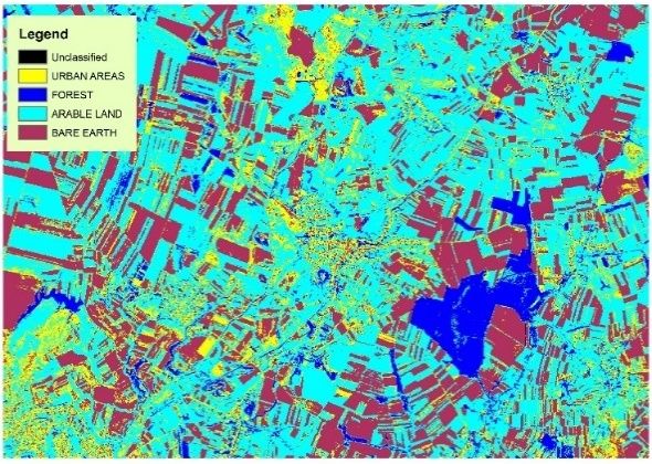
JOURNAL OF APPLIED ENGINEERING SCIENCES VOL. 10(23), ISSUE 2/2020
ISSN: 2247-3769 / e-ISSN: 2284-7197 ART.NO. 299 pp. 163-172
distance (Navalgund, 2001). The first images from space were When talking about digital images characteristics, four types of
taken on the sub-orbital V-2 rocket flight, launched by the resolutions are important. Spatial resolution represents the size
United States, in the year 1946 (Fig. 2). of the section of the Earth’s surface which can be depicted in
one pixel and radiometric resolution indicates the ability of the
sensor to distinguish between grey-scale values and is measured
in bits.
Dealing with thematic applications, spectral resolution indicates
how well a spectral-digital sensor can distinguish between the
different spectral ranges of the electromagnetic spectrum and
the temporal resolution indicates the distance in time between
two successive image acquisitions of the same area.
To view and analyse satellite images, a pre-processing is needed
to remove the atmospheric effect (Fig. 3), correct the radiometry
and improve the geometric properties.
Figure 2. Image of Earth from Space
(First photo from space, 2020)
The concept of satellite imagery refers to digitally transmitted
images taken by artificial satellites orbiting the Earth. The first
successful weather satellite, Tiros-1, was launched by the
National Aeronautics and Space Administration (NASA). It
transmitted infrared images of Earth’s cloud cover and was able
to detect and chart hurricanes. In 1972, NASA launched the
Earth Resources Technology Satellite; this was the start of the
longest-running program of satellite imagery of the Earth, later
renamed Landsat.
Figure 3. Example of simulated Sentinel-2 data before and after
Landsat instruments acquire millions of images that are used to atmospheric correction (Sentinel 2, 2012)
evaluate natural and human changes of the Earth. Landsat 8 was
launched in 2013 and has two sensors on-board: Operational 3. OVERVIEW ON CLASSIFICATION PROCESSES
Land Imagery (OLI) and Thermal Infrared Sensor (TIRS).
Landsat 8 measures in 11 ranges of frequencies along the One of the main application of aerial and satellite images is the
electromagnetic spectrum and the products have three different classification for land cover information extraction (Kramer,
spatial resolutions: 15 meters (panchromatic), 30 meters 2002), (Foody and Mathur, 2004).
(visible, near-infrared and short-wavelength infrared) and 100 m
(thermal) (Landsat Program, 2020). Image classification is the process of grouping pixels into
several classes of land use or land cover, based on statistical
The European Space Agency (ESA) developed a new family of decision rules in the multispectral domain or logical decision
satellites in the Copernicus program. These missions carry a rules in the spatial domain. The methods and the algorithms
range of technologies (radar and multispectral imaging) for used in the classification process are called image classifiers
monitoring land, ocean, and atmosphere. Sentinel-1 is a radar (Kamavisdar et al., 2013). The classification process consists of
imaging mission for land and ocean services. Sentinel-2 is a the following steps:
multispectral imaging mission for land monitoring to provide,
for example, imagery of vegetation, soil and water cover, inland Pre-processing: analysing the input data by
waterways and coastal areas. interpreting and understanding it and defining the
number of classes for classification;
Sentinel-3 is a multi-instrument mission to measure sea-surface Training: creating the samples for each class used for
topography, sea- and land-surface temperature, ocean color and the training and the validation step.
land color with high-end accuracy and reliability. Sentinel-5P Applying the image classifier: running the desired
provides timely data on a multitude of trace gases and aerosols classification methods.
affecting air quality and climate. Sentinel-4 and Sentinel-5 are Post classification: assessment of accuracy (Foody,
payload devoted to atmospheric monitoring. Finally, Sentinel-6 2002).
carries a radar altimeter to measure global sea-surface height,
primarily for operational oceanography and climate studies The classification process (Fig. 4.) is categorized, in supervised
(Sentinel 2, 2012). Nowadays various space agencies and and unsupervised classification, based on the use or not of
satellite product providers have adopted a free and unrestricted training samples. In the next paragraphs the most common
data access policy for satellite data. We can recall here, the classifiers are presented.
Copernicus program (ESA), over five million Landsat images
from 1972 onwards (U.S. Geological Survey), the 30 meters
Digital Elevation Models (Japan Aerospace Exploration Agency
and NASA), etc.
165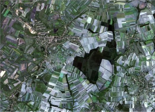
JOURNAL OF APPLIED ENGINEERING SCIENCES VOL. 10(23), ISSUE 2/2020
ISSN: 2247-3769 / e-ISSN: 2284-7197 ART.NO. 299 pp. 163-172
3.2 MLC
Maximum Likelihood Classifier - MLC (Duda and Hart, 1973),
also called Discriminant Analysis, is the most popular statistical
method of classifying images. According to this approach, a
pixel with the maximum likelihood is classified into the
corresponding class. The steps involved in MLC process are the
following:
computing the parameters that represent the data
(standard deviation, sigma, mean, etc.), for each class;
computing the probability density of every feature
vector to each class, based on the parameters
calculated in the prior step;
Figure 4. Types of image pixel-based classification finding the maximum of all the computed probability
densities for each class. The class with the parameters
3.1 SVM that give the maximum probability is the predicted
class of the data point.
Support-Vector Machine (SVM) algorithm has its roots in
Statistical Learning Theory (Vapnik, 1995). SVM is a A simplified version of this classifier is given in equation (1).
supervised learning model with associated learning algorithms
that analyse the data used for classification. In the beginning, 1
given a set of training samples, each marked as belonging to one | = (1)
or the other of two classes, SVM training algorithm built a √2
model that assigns a label to every pixel, as belonging to one of
the classes, making it a non-probabilistic binary linear classifier. where:
ωj = set of parameters for each class j;
The characteristic that defines the SVM classifier is that its σj = standard deviation for the class j;
purpose is to find a hyperplane (Fig. 5 and 6.) in an N- μj = mean for the class j;
dimensional space (N is the number of features), that distinctly x = feature vector.
classifies the data points (Gandhi, 2018).
The standard deviation and the mean of every class are used as
Hyperplanes are decision boundaries that help to classify the parameters, but with the MLC model other parameters can be
data points, that is, data points falling on either side of the used as well. In equation (1) the correlation between features is
hyperplane are attributed to different classes. Also, the neglected. The full version of MLC, implemented in remote
dimension of the hyperplane depends upon the number of sensing software, is described by equation (2).
features. If the number of classes is two, then the hyperplane is
just a line, if the number of input features is three, then the ( )=− | |−( − ) ( − ) (2)
hyperplane becomes a plane. It becomes difficult to imagine
where:
when the number of features exceeds 3.
= sum of all standard deviations ;
( − ) ( − ) = Mahalanobis Distance.
An advantage of using the Mahalanobis distance is that it takes
into consideration the correlation between classes. When using
MLC a sufficiently large ground truth sampled data is required
to allow the estimation of the unknown parameters.
3.3 Accuracy assessment
Accuracy assessment is an important part of any classification
process. In this step, the classified image is compared to a data
Figure 5. Hyperplanes in 2D space (Gandhi, 2018) source that is considered the ground truth data. Ground truth can
be collected in the field or can be derived from interpreting
high-resolution imagery, from existing classified imagery, or
from existing GIS data layers.
The relationship between the known reference data (ground
truth) and the corresponding results of the classification
procedure is stored in the confusion matrix. The accuracy
indicators are then computed based on this matrix.
Figure 6. 2D and 3D hyperplanes (Gandhi, 2018)
166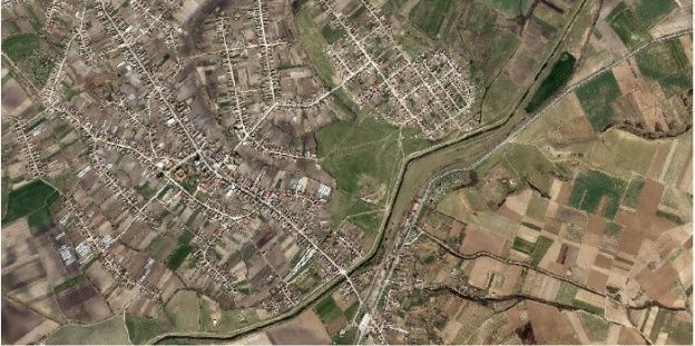
JOURNAL OF APPLIED ENGINEERING SCIENCES                                                                       VOL. 10(23), ISSUE 2/2020
ISSN: 2247-3769 / e-ISSN: 2284-7197                                                                            ART.NO. 299 pp. 163-172

Overall Accuracy describes the percentage of correctly                using two different classifiers and the comparison of the results
classified pixels from the total number of reference pixels.          are presented.
The Kappa Coefficient is generated from a statistical test to
evaluate the accuracy of the classification. Kappa evaluates how      4.1 Classification of orthophotos
well the classification performed as compared to just randomly
assigning classes. The values can range from -1 to 1. A value of      The first type of image data was acquired during a
0 indicates that the classification is no better than a random one.   photogrammetric aerial flight within the project LAKI II, that
A value close to 1 indicates that the classification is better than   started in 2017 (Fig. 8.) and covers an area of 50.000 km2 in the
random.                                                               western and central part of Romania. For the acquisition of
                                                                      aerial images the UltraCam Eagle Prime camera was used,
Errors of omission refer to reference samples that were left out      mounted on a Twin Commander 690A airplane. For image
(or omitted) from the correct class in the classified map. To         classification, a true-color (RGB) orthophoto with ground
compute the omission for every class, the incorrect                   resolution 20 centimeters and a planimetric accuracy of 30
classifications are added and divided by the total number of          centimeters was used (Fig. 9).
reference samples.

Errors of commission are calculated by reviewing the
classified samples for incorrect classifications. This is done by
adding together the incorrect classifications and dividing them
by the total number of classified samples for each class.

Producer's Accuracy is the map accuracy of the mapmaker
(the producer) and represents how often real features on the
ground are correctly shown on the classified map. It is                 Figure 8. Area for LAKI II Project and the photogrammetric
calculated as the number of correctly classified pixels divided                       camera used for data acquisition
by the total number of reference pixels for that class.

The User's Accuracy is the accuracy for a map user and is
referred to as reliability. It indicates how often the class on the
map will be present on the ground. The User's Accuracy is
calculated by dividing the total number of correctly classified
pixels for a class by the number of pixels that were classified in
that class.

                       4. CASE STUDY

The area chosen for the tests is located in Săcueni City in Bihor        Figure 9. Aerial orthophoto used for image classification
County, Romania (Fig. 7).
                                                                      The first step in the classification process was image
                                                                      interpretation in order to configure the classes to be extracted.
                                                                      Based on the land use and land cover characteristics, the
                                                                      following classes were selected: BUILDINGS, ROADS,
                                                                      GRASS, BARE-EARTH and WATER.

                                                                      In ENVI 5.3 software, the samples were digitized for training
                                                                      and reference (Table 1). These samples must be uniformly
                                                                      distributed across the image (as far as possible) and must
                                                                      contain the most representative areas for the corresponding class
                                                                      (Fig. 10). As classifiers, both SVM and MLC.

                                                                                           Training dataset       Reference dataset
                                                                          Classes
                                                                                            No.          No.        No.          No.
                                                                                          polygons      pixels    polygons      pixels
                                                                        BUILDINGS             20        11456         15         10319
                                                                          ROADS               14        17380         12         17239
                                                                          GRASS               15        39574         15         41472
                                                                       BARE-EARTH             15        50561         15         58401
                                                                         WATER                 5        10590          5         13099
                Figure 7. Săcueni City, Romania
                                                                       Table 1. Number of samples for training and reference dataset
The study case analyses the results achieved in image
classification using two different sources of data, from airborne
and satellite platforms. In the next paragraphs the input data, the
corresponding products obtained, the results of the classification

                                                                                                                                     167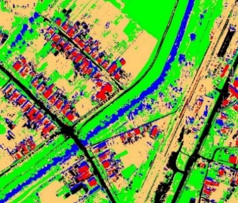
JOURNAL OF APPLIED ENGINEERING SCIENCES                                                                   VOL. 10(23), ISSUE 2/2020
ISSN: 2247-3769 / e-ISSN: 2284-7197                                                                        ART.NO. 299 pp. 163-172

                                                                   classifier the pixels that are classified as BUILDINGS represent
                                                                   3.61% from the total amount of pixels, but when applying the
                                                                   MLC classifier the BUILDINGS percentage increases to
                                                                   23.18%. From a visual analysis, the SVM classifier seems to
                                                                   offer better results in the classification process.

                                                                   A detailed view of the classification on the city of Săcueni is
                                                                   shown in Fig. 13, where the water bodies are displayed with
                                                                   blue colour and the roads are shown in black. From a visual
                                                                   qualitative inspection, these two classes seem well extracted
                                                                   from the image; after applying successive aggregations, noisy
                                                                   pixels can be removed.
   Figure 10. Example of samples digitized for classification

After training the classifiers on the training dataset, the
algorithm was applied to the input data; the results of the
classification using SVM and MLC are displayed in Fig. 11 and
Fig 12.

                                                                    Figure 13. A detailed view of the results with SVM classifier

                                                                   The final step in the classification process was the accuracy
                                                                   assessment based on the reference dataset previously classified.
                                                                   For the SVM classifier, the overall accuracy is 97.6% and the
                                                                   Kappa coefficient is 0.97. The corresponding confusion matrix
                                                                   is displayed in Table 2. The classes ROADS and BARE-
                                                                   EARTH generate confusion in the classification process, which
                                                                   is probably due to the fact that the classification is performed
              Figure 11. SVM classification result                 only using the RGB bands. For the MLC classifier, the overall
                                                                   accuracy is 97.2% and the Kappa coefficient is 0.96, so slightly
                                                                   lower than the SVM result.

                                                                            Ref.                                  Bare
                                                                                   Buildings   Roads    Grass               Water
                                                                                                                  Earth
                                                                   Train.
                                                                      Buildings     10769        0        0        400        0
                                                                       Roads          0        18003      1        2737       0
                                                                       Grass          0          0      42927       0         1
                                                                     Bare Earth      196        104       12      56942       61
                                                                       Water          32         0        0         0       13533

                                                                             Table 2. Confusion matrix, SVM classifier

                                                                   From the accuracy indicators summarized in Fig. 14, it can be
                                                                   concluded that the GRASS class has been well classified. The
                                                                   producer and user accuracies are comparable for all classes
                                                                   using the two classifiers, except for the BUILDINGS class
                                                                   where significant differences are present.

              Figure 12. MLC classification result

The percentages for pixels belonging to different classes differ
greatly for the class BUILDINGS. When using the SVM

                                                                                                                                 168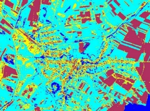
JOURNAL OF APPLIED ENGINEERING SCIENCES                                                                    VOL. 10(23), ISSUE 2/2020
ISSN: 2247-3769 / e-ISSN: 2284-7197                                                                         ART.NO. 299 pp. 163-172

                                                                   From the indicators in Table 4, the minimum errors are obtained
                                                                   for the GRASS class and the maximum errors occur for the
                                                                   BARE-EARTH 3 class. So, we can concluded that this
                                                                   approach didn’t improve the previous classification results.

                                                                         Class /      Comm.     Omis.      Producer      User
                                                                        Accuracy      Error     Error      Accuracy   Accuracy
                                                                        Indicator         Percent                Percent
                                                                         ROADS         14.88       6.48       93.52        85.12
                                                                       BUILDINGS       9.55       36.72       63.28        90.45
                                                                         GRASS         2.35        2.91       97.09        97.65
                                                                      BARE-EARTH 1     22.42      25.27       74.73        77.58
                                                                      BARE-EARTH 2     40.75      39.37       60.63        59.25
                                                                         WATER         21.68       5.03       94.97        78.32
                                                                         TRESS         46.14      52.33       47.67        53.86
                                                                      BARE-EARTH 3     85.9       75.46       24.54         14.1

   Figure 14. Comparison of the accuracy indicators for the        Table 4. Accuracy assessment using the MLC approach for the
       classification of the orthophoto of Săcueni city                dataset with 8 classes (the best results are highlighted)

To test if more classes would improve the results of the           4.2 Classification of Sentinel Images
classification, three classes were added to the previous ones,
two for different types of BARE-EARTH and one for TREES.           The second image dataset on the city of Săcueni tested for
Table 3 summarizes the number of samples for each class for        classification was acquired by Sentinel-2A MSI sensor (Fig. 16)
both datasets (training and reference).                            on 30.08.2019. The data was downloaded from https://scihub.
                                                                   copernicus.eu/.
                     Training dataset       Reference dataset
     Classes          No.          No.       No.         No.
                    polygons     pixels    polygons     pixels
  BUILDINGS            35        16086        35        15545
    ROADS              30       102646        30       110799
    GRASS              30       276212        30       276584
BARE-EARTH 1           36        23555        36       259188
BARE-EARTH 2           23       162953        23       151923
BARE-EARTH 3            9        36681         9        39243
    TREES              13        54649        13        49924
   WATER               20         9407        20        84348

Table 3. Number of samples for training and reference dataset,           Figure 16. Sentinel-2 (“Sentinel 2, a valuable tool in
                    when using 8 classes                                            environmental studies”, 2017)
The classification algorithm chosen for this approach was MLC      The Copernicus Sentinel-2 mission comprises a constellation of
(Fig. 15) that is expected to perform better for a larger number   two polar-orbiting satellites placed in the same sun-synchronous
of classes. The result for the overall accuracy is 76.1% and the   orbit, phased at 180° to each other.
Kappa coefficient is 0.69.
                                                                   It aims at monitoring Earth's surface changes and has a wide
                                                                   swath width (290 km) and high revisit time (5/10 days). It
                                                                   carries an optical instrument payload that samples 13 spectral
                                                                   bands, with the following spatial resolutions: 10 meters (4
                                                                   bands), 20 meters (6 bands) and 60 meters (3 bands). Sentinel-2
                                                                   products available for users are at two different levels: 1C and
                                                                   2A (https://sentinel.esa.int). Level-1C products provide the top
                                                                   of atmosphere reflectances in fixed cartographic geometry, so
                                                                   the radiometric and geometric corrections are applied. Level-2A
                                                                   products provide the bottom of atmosphere reflectance in a
                                                                   geospatial reference system. This product is atmospherically
                                                                   corrected, based on the libRadtran radiative transfer model
                                                                   (Mayer, 2005), using the Sen2Cor processor and PlanetDEM
                                                                   Digital Elevation Model. In this work images with Level 2A
                                                                   were used.

                                                                   The downloaded files contain 13 different images, one for each
                                                                   spectral band. For classification the four bands in the visible and
                                                                   near-infrared spectrum with ground resolution of 10 meters
                                                                   were used (Fig. 17).
         Figure 15. MLC classification with 8 classes

                                                                                                                                   169
JOURNAL OF APPLIED ENGINEERING SCIENCES                                                                     VOL. 10(23), ISSUE 2/2020
ISSN: 2247-3769 / e-ISSN: 2284-7197                                                                          ART.NO. 299 pp. 163-172

       Figure 17. Satellite imagery over the city Săcueni

In the process of image interpretation, five classes were defined:
urban area, forest, arable land, bare earth and roads; as for the
airborne case, SVM and MLC classifiers were applied. For the
training dataset, 70 samples were used, the same as for the
reference set (Fig. 18).
                                                                            Figure 20. MLC classification of Sentinel-2 image

                                                                     For the SVM classifier, the pixels classified as URBAN
                                                                     AREAS and FOREST increased inversely proportionally, if
                                                                     compared to the MLC classifier.

                                                                     The results of the classification process for the city of Săcueni
                                                                     are visualized in Fig. 21. By a visual check, it can be confirmed
                                                                     that the pixels classified in the ROADS class with SVM are
                                                                     more than those classified with MLC.
       Figure 18. Statistics samples for the satellite image

The application of the SVM and MLC classifiers following the
training process led to the results presented in Fig. 19 and Fig
20. The results are showing that for ROADS class, the MLC
ranks more pixels than SVM, but after the visual inspection we
can state that not all ROADS pixels are well classified.

                                                                     Figure 21. Comparison between the results obtained from MLC
                                                                                  and SVM classification algorithms

                                                                     The accuracy assessment executed in the post-classification
                                                                     process with the reference dataset, produced the confusion
                                                                     matrix and the indicators, showing that the indistinctness
                                                                     between the classes that led to the result of the classification.
                                                                     The accuracy indicators are computed for each class and
                                                                     summarized in Fig. 22. The ROADS class has the worst results
                                                                     in the classification process. The producer and user accuracies
                                                                     are comparable for most of the classes for both classifiers,
                                                                     except for the ROADS class where bigger differences are
                                                                     evident.

       Figure 19. SVM classification of Sentinel-2 image

                                                                        Figure 22. Comparison of the accuracy indicators for the
                                                                                     satellite image of Săcueni city

                                                                                                                                   170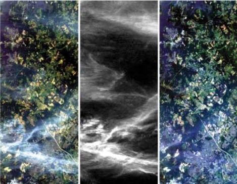
JOURNAL OF APPLIED ENGINEERING SCIENCES                                                                     VOL. 10(23), ISSUE 2/2020
ISSN: 2247-3769 / e-ISSN: 2284-7197                                                                          ART.NO. 299 pp. 163-172

Based on the results shown, it was decided to eliminate the class
ROADS from the classification process. The image was re-
interpreted and configured on four classes (URBAN AREAS,
FOREST, ARABLE LAND and BARE EARTH). From the
available 144 samples, 40% were used in the training dataset
and 60% in the reference dataset.

The results obtained from the new training dataset on the same
satellite image, and applying the same two algorithms, are
shown in Fig. 23 and Fig. 24. The approach using MLC gives            Figure 24. MCL classification result for the satellite image,
an overestimated result for URBAN AREAS class, with a                                  when using 4 classes
growth of about 11% if compared with the approach using SVM
(Fig. 24).

The accuracy indicators calculated using the reference dataset
show that by reducing the number of classes the results are
more precise, both visually and numerically.

Also, in the case of satellite images, based on the accuracy
assessment summarized in Fig. 25, SVM classifier performs a
better classification than MLC classifier.

                                                                    Figure 25. Accuracy assessment for classification of the satellite
                                                                                  image over Săcueni city (4 classes)

                                                                    The final classification result of the SVM classifier on Sentinel-
                                                                    2A image on Săcueni city is shown in Fig. 26. After a visual
                                                                    inspection, it can be concluded that these classes are properly
                                                                    extracted.

  Figure 23. SVM classification result for the satellite image,
                   when using 4 classes
                                                                    Figure 26. Results obtained for SVM classification algorithms,
                                                                                           for Săcueni city

                                                                                         5. CONCLUSIONS

                                                                    In this paper it is shown that by using more classes and samples
                                                                    on the aerial orthophoto, the result of the classification does not
                                                                    improve, but more confusion between classes appear and the
                                                                    likelihood of an object being in the corresponding class is
                                                                    reduced. For the SVM classifier, a smaller number of classes
                                                                    and samples gives the best results for the classification.
                                                                    Subsequently, the results can be post-processed to obtain an
                                                                    image with higher accuracy per class and less noise in the data.
                                                                    Therefore it can be concluded that the SVM classifier, for both
                                                                    images used in the case study, offers higher accuracy in the
                                                                    classification process. For extra-urban areas or large areas it is

                                                                                                                                   171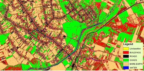
JOURNAL OF APPLIED ENGINEERING SCIENCES                                                                         VOL. 10(23), ISSUE 2/2020
ISSN: 2247-3769 / e-ISSN: 2284-7197                                                                              ART.NO. 299 pp. 163-172

most likely to use satellite images, but for urban areas or small     Wolf, P. R., Dewitt, B. A., Wilkinson, B. E., 2014. Elements of
areas, the aerial images with appropriate spatial resolution are      Photogrammetry with Application in GIS. McGraw-Hill Education,
the best choice. The results of classification depend on the          4th Edition, New York.
distribution and completeness of the datasets used for training       Vreys, K., Iordache, M. D., Bomans, B., Meuleman, K., 2016. Data
and as reference and on the number of classes chosen.                 acquisition with the APEX hyperspectral sensor. Miscellanea
                                                                      geographica – regional studies on development, 20 (1), pp. 5-10,
The confusion matrix can offer valuable information about the         https://doi.org/10.1515/mgrsd-2016-0001.
classes with similar features, so the classes that create confusion
can be eliminated from the process, or the corresponding              Duda, R., Hart, P., 1973. Pattern classification and scene analysis.
samples can be edited (if possible). The processing time in           A Wiley-Interscience publication.
ENVI software is less for the MLC classifier than for SVM one.        Linder, W., 2006. Digital Photogrammetry A Practical Course.
To extract objects from the classified images the workflow has        Springer, New York.
to be extended; in fact the two classifiers are pixel-based and
the accuracy indicators refer to the pixel, not to the object.        Kramer, J. H., 2002. Observation of the earth and its environment:
                                                                      Survey of missions and sensors, 4th Edition.
                                                                      Schenk, T., 2005. Introduction to Photogrammetry. Department of
                                                                      Civil and Environmental Engineering and Geodetic Science, Ohio
                6. ACKNOWLEDGEMENTS                                   State University, pp. 3-4.
                                                                      Vapnik, V. N., 1995. The Nature of Statistical Learning Theory.
The authors thank the National Centre of Cartography and the          Information Science and Statistics. Springer-Verlag.
National Agency of Cadastre and Land Registration for                 “HySpex”, https://www.hyspex.com (view at 10 August 2020).
providing the aerial imagery, the colleagues from the University
of Warsaw, partners in the VOLTA project (Grant Agreement             “DigitalGlobe”, http://worldview3.digitalglobe.com      (view at 11
no. 734687 — VOLTA — H2020-MSCA-RISE-2016) who                        August 2020).
provided with the ENVI licenses used for the classification           “Boston as the eagle and the wild goose                     see     it”,
process. Finally, the authors acknowledge ESA for the Sentinel        http://bit.ly/2m6wgXa (view at 30 August 2020).
dataset.
                                                                      “Aerial Photography and Remote Sensing”, last modified
                                                                      September                        11,                      2014,
                                                                      https://web.archive.org/web/20141030095245/http://www.colorado.
                                                                      edu/geography/gcraft/notes/remote/remote_f.html.
References:
                                                                      “First photo from space”, last edited March 27, 2020,
Foody, M. G., 2002. Status of Land Cover Classification Accuracy      https://commons.wikimedia.org/wiki/File:First_photo_from_space.j
Assessment, Remote Sensing of Environment, 80, pp. 185-201.           pg.
Foody, M. G., Mathur, A., 2004. A Relative Evaluation of              “Landsat Program”, https://landsat.gsfc.nasa.gov (view at 03
Multiclass Image Classification by Support Vector Machines. IEEE      September 2020).
Transactions on Geoscience and Remote Sensing, 42, pp. 1335 –
1343.                                                                 “Sentinel 2”, Copyright © 2012 European Space Agency,
                                                                      https://sentinel.esa.int/documents/247904/349490/S2_SP-
Karbo, N., Schroth, R., 2009. Oblique aerial photography: a status    1322_2.pdf.
review. Proc. 52nd Photogrammetric Week, pp. 119-125.
                                                                      Gandhi, R., “Machine learning algorithms”, last modified June 7,
Kamavisdar, P., Saluja, S., Agrawal, S., 2013. A Survey on Image      2018,       https://towardsdatascience.com/support-vector-machine-
Classification Approaches and Techniques. International Journal of    introduction-to-machine-learning-algorithms-934a444fca47.
Advanced Research in Computer and Communication Engineering,
                                                                      “Sentinel”, https://sentinel.esa.int (view at 03 September 2020).
2 (1).
Leberl, F., Thurgood, J., 2004. The Promise of Softcopy               “Sentinel 2, a valuable tool in environmental studies”, last modified
                                                                      March 4, 2017, https://www.cls.fr/en/sentinel-2-environmental-
Photogrammetry Revisited. Theme Session 12: Automated Object
                                                                      studies.
Extraction and Computer Vision Application.
Lemmens, M., 2011. Digital aerial cameras. GIM International,
25(4).
Mayer, B., Kylling, A., 2005. Technical note: The libRadtran soft-
ware package for radiative transfer calculations– description and
examples of use, Atmos. Chem. Phys., 5, pp. 1855–1877,
doi:10.5194/acp-5-1855.
Navalgund, R. R., 2001. Remote sensing. Reson, 6, pp. 51-60,
https://doi-org.am.e-nformation.ro/10.1007/BF02913767.
Petrie, G., 2009. Systematic aerial oblique photography using
multiple digital cameras. Photogrammetric Engineering & Remote
Sensing, pp. 102-107.
Remondino, F., Rupnik, E., Nex, F., 2014. Oblique Multi-Camera
Systems - Orientation and Dense Matching Issues. ISPRS, XL-
3/W1.

                                                                                                                                            172
You can also read