Undefined class-label detection vs out-of-distribution detection
←
→
Page content transcription
If your browser does not render page correctly, please read the page content below
Undefined class-label detection vs out-of-distribution
                                                                  detection

                                                                    Xi Wang                                   Laurence Aitchison
                                                     School of Data Science and Engineering              Department of Computer Science
                                                         East China Normal University                          University of Bristol
arXiv:2102.12959v2 [stat.ML] 29 May 2021

                                                                Shanghai, China                                    Bristol, UK
                                                              xidulu@gmail.com                          laurence.aitchison@gmail.com

                                                                                            Abstract

                                                       We introduce a new problem, that of undefined class-label (UCL) detection. For
                                                       instance, if we try to classify an image of a radio as cat vs dog, there will be no
                                                       well-defined class label. In contrast, in out-of-distribution (OOD) detection, we are
                                                       interested in the related but different problem of identifying regions of the input
                                                       space with little training data, which might result in poor classifier performance.
                                                       This difference is critical: it is quite possible for there to be a region of the input
                                                       space where little training data is available but where class-labels are well-defined.
                                                       Likewise, there may be regions with lots of training data, but without well-defined
                                                       class-labels (though in practice this would often be the result of a bug in the
                                                       labelling pipeline). We note that certain methods originally intended to detect OOD
                                                       inputs might actually be detecting UCL points and develop a method for training
                                                       on UCL points based on a generative model of data-curation originally used to
                                                       explain the cold posterior effect in Bayesian neural networks. This approach gives
                                                       superior performance to past methods originally intended for OOD detection.1

                                           1       Introduction
                                           Many neural networks are trained on restricted datasets (e.g. MNIST includes only images of
                                           handwritten digits), and may fail if applied outside of that restrictive setting. It is therefore important
                                           to be able to distinguish between data points in the training distribution and out of distribution (OOD).
                                           This can be achieved for instance by training a generative model of the inputs, and asking whether
                                           any given test-input has high-probability under that model (Wang et al., 2017; Pidhorskyi et al., 2018,
                                           and see Related Work for further details).
                                           However, there are now many methods to train classifiers that generalise well to OOD data (Arjovsky
                                           et al., 2019; Ahuja et al., 2020; Krueger et al., 2020). If we use such a classifier, then detecting OOD
                                           points and ignoring our classifier’s predictions on those points becomes potentially undesirable: we
                                           might ignore predictions in OOD regions where the classifier performs well. In this context, OOD
                                           detection is clearly problematic, but we still want to detect nonsense inputs which do not have a
                                           sensible class label. We consider this new problem, undefined class-label (UCL) detection.
                                           To get an understanding of how OOD points differ from UCL points, consider MNIST (LeCun
                                           et al., 1998), containing images of handwritten digits (Fig. 1A left) which can be classified using 0–9
                                           class labels. There are many input images that are clearly OOD for MNIST but could be classified
                                           meaningfully with the same 0–9 class labels (Fig 1A middle). An example comes from the corrupted
                                           MNIST dataset (Mu & Gilmer, 2019, Apache License 2.0), which was explicitly designed to be
                                           OOD if we take MNIST to be the training dataset. In contrast, there are other OOD images without a
                                               1
                                                   Code at: anonymous.4open.science/r/58f3/; MIT Licensed

                                           Preprint. Under review.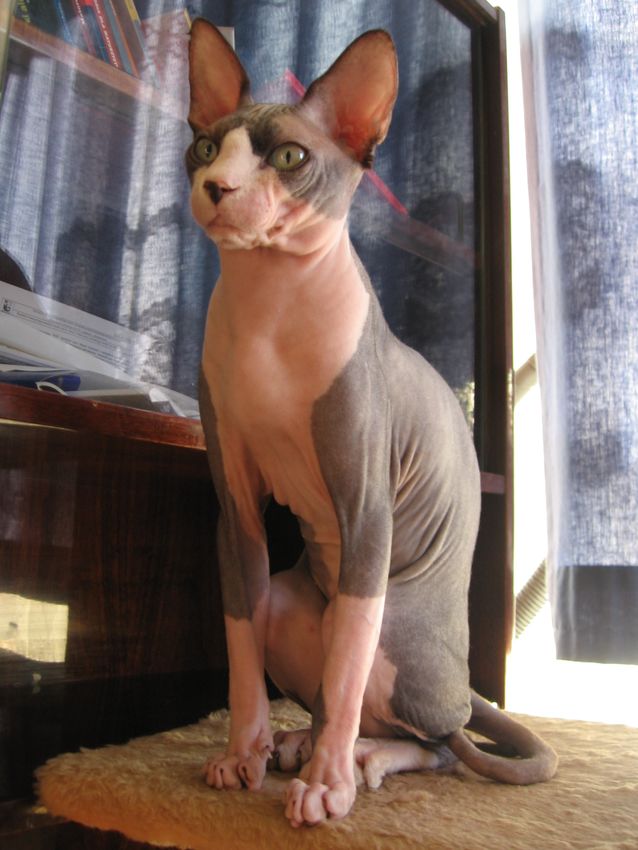
(A)                                                       (B)
            Training set     Well-defined Undefined                   Training set      Well-defined Undefined
                                OOD         OOD                                            OOD        In-dist

Figure 1: (A) When training on MNIST (left), there is the potential for OOD images with a well-
defined class-label (middle), and for images that simultaneously are OOD and have a UCL (right).
(B) Consider accidentally asking human annotators to label EMNIST with the digits 0–9. EMNIST
contains images of digits, but also uppercase and lowercase letters (left). As such, there are OOD
images with well-defined class-labels (middle), as in Fig. 1A. But there are now in-distribution images
with UCLs (right).

Figure 2: A schematic figure visualising three different types of samples: OOD samples (grey ‘x‘ on
the left), in-distribution samples with well-defined labels (red and blue clusters in the middle) and
in-distribution samples with UCLs (right most cluster of mixed blue and red points). The underlying
distribution for in-distribution samples is a three-component Gaussian mixture whose density is
shown by the colormap, with darker color indicating larger density.

well-defined 0–9 class label (such as a handwritten letter “W”; Fig 1A right). Here, our goal is to
detect input points without a well-defined class label, and this is the UCL detection problem.
Further, note that it is possible for points to be in-distribution, but have UCLs. For instance, consider
asking annotators to classify images as digits (0–9), but accidentally presenting them with images
from EMNIST (Cohen et al., 2017, Fig 1B left) rather than MNIST. EMNIST contains a mixture
of digits and upper and lowercase alphabetic characters, so there are some in-distributions images
with a well-defined class-label (i.e. images of digits) and other in-distribution images with UCLs
(i.e. those of letters; Fig 1B right). When an annotator is presented with a UCL image, all they
can do is to respond with a random label. As before, there are also OOD images with well-defined
class-labels (Fig 1B middle). We can additionally illustrate this case via a toy dataset (Fig 2), which
has an in-distribution region on the right where there are no well-defined class-labels and so red and
blue points are intermixed.
In addition, OOD vs UCL detection is an important consideration when working with well-calibrated
classifiers that give good uncertainty estimates. For poorly calibrated classifiers that are incapable of
reasoning about uncertainty, OOD detection is clearly desirable as the classifier may give nonsense

                                                      2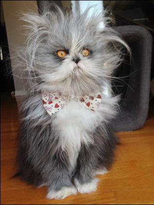
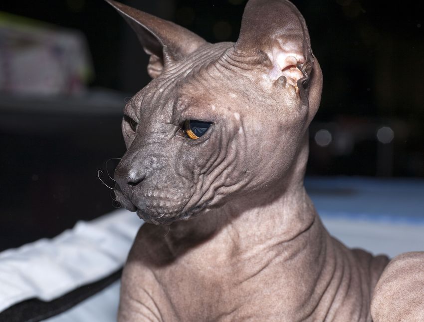
Figure 3: Classifying these images as cats vs dogs has a well-defined right answer; the pictured
animals are either a dog or a cat and an expert human annotator would be able to distinguish them.
However, a machine learning algorithm or even an untrained human annotator may have epistemic
uncertainty (i.e. they may be unsure about the class-label because they have not seen enough training
data). As such, the existence of epistemic uncertainty does not imply that the images have UCLs (but
epistemic uncertainty remains a good heuristic to find regions of input space with little training data).
Left: a sphynx cat. Middle: a Persian cat with congenital hypertrichosis. Right: a Donskoy cat.

     Y1 = Y2 = Y3 = cat                Y1 = Y2 = Y3 = dog            Y1 = Y2 = dog;      Y3 = cat
            Y = cat                          Y = dog                         Y = Undef

Figure 4: An example of the generative model of dataset curation, with S = 3. Three annotators
are instructed to classify images as cats or dogs. The left and middle images have well-defined
class-labels as they are clearly a cat and a dog respectively. Therefore, the annotators all give the
same answer and consensus is reached. However, the right-most image has a UCL, so the annotators
are forced to give random answers; they disagree and we remove the image from the dataset.

answers far from the training data. However, for well-calibrated classifiers that are capable of
reasoning about uncertainty, it may well be the case that we care more about detecting UCL inputs
than OOD inputs. In particular, consider an OOD point with a well-defined class label, such as those
in Fig 1A middle. These images are clearly OOD, and indeed were explicitly designed to be OOD (Mu
& Gilmer, 2019). At the same time, Mu & Gilmer (2019) show that simple convolutional classifiers
trained on MNIST perform well above chance on these datasets (67.17% test accuracy). As such, a
well-calibrated classifier should return an uncertain predictive distribution that is nonetheless highly
informative about the true class label. This is useful information that should not be thrown away by
declaring the point OOD. Even in the case that the distribution is highly uncertain (perhaps even close
to uniform), as long as the downstream processing pipeline takes this uncertainty into account when
making decisions, there would seem to be little benefit in additionally declaring the point OOD. In
contrast, identifying UCL points is always desirable because even a uniform distribution over classes
does not make sense for a UCL point because the underlying image fundamentally does not depict
one of the limited range of classes.
To operationalise the notion of UCL, we need to understand how points with well and undefined
labels might be labelled by human annotators. When labelling points with a well-defined class-label,
different annotators will be highly consistent: almost always giving the same answer for each image.
However when forced to label a UCL image, all the annotator can do is to give a random answer, and
this is unaffected by annotator expertise or the amount of training data. Thus, a UCL image can be
identified by asking multiple annotators to label it and looking for disagreements. Interestingly, this
corresponds to aleatoric uncertainty or output noise, rather than epistemic uncertainty (which is more
suited to detecting OOD points, see Related Work).
In addition to introducing UCL detection and distinguishing it from OOD detection, we give methods
for solving the UCL detection problem using a principled statistical model describing the probability
of disagreement amongst multiple annotators. This model was originally developed to explain

                                                   3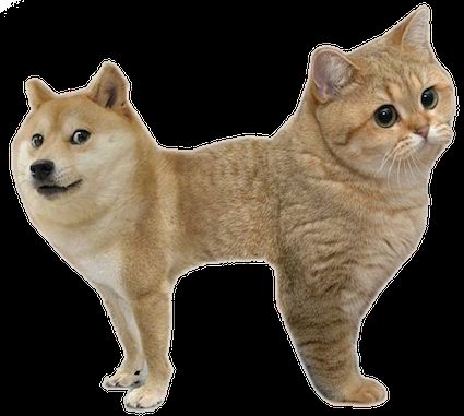
the cold-posterior effect in Bayesian neural networks (Aitchison, 2021), and was later used to
understand semi-supervised learning (Aitchison, 2020). As this is a principled statistical model, we
are additionally able to give a principled maximum-likelihood method for training on UCL points.

2   Related work

While OOD and UCL detection might seem to have much in common, probabilistic approaches to
their solution are radically different. In particular, it is possible to solve the OOD detection task by
fitting a generative model of inputs, and declaring inputs with low probability under that model as
OOD (Wang et al., 2017; Pidhorskyi et al., 2018 though there are considerable subtleties in getting
this approach to work well Nalisnick et al., 2018; Choi et al., 2018; Shafaei et al., 2018; Hendrycks
et al., 2018; Ren et al., 2019; Morningstar et al., 2020).
In contrast, generative modelling of the inputs is not a valid approach to UCL detection. As we saw
above, it is quite possible for there to be little training data in a region with well-defined class labels
(e.g. Fig. 1A middle). Likewise, it is possible for there to be lots of training data in a region without
well-defined class-labels (e.g. Fig. 1B) which should be more unusual, but might emerge due to an
error in a semi-automated labelling pipeline.
There are other probabilistic approaches to the OOD problem based on epistemic uncertainty. Broadly
speaking, these approaches fit a Bayesian posterior approximation for the neural network parameters
(for the purposes of this discussion we include ensembles Lakshminarayanan et al., 2016; Pearce et al.,
2018; Milios et al., 2020). Different setting of the parameters sampled from the Bayesian posterior
will give different predictive distributions at any given test point. Importantly, we would expect these
predictive distributions to differ dramatically in regions far from the training data (indicating high
epistemic uncertainty) and the predictive distributions to all be very similar when close to the training
data (indicating low epistemic uncertainty; Lakshminarayanan et al., 2016; Kendall & Gal, 2017).
Ultimately, this is typically conceived of as a heuristic for finding regions of the input space which
are OOD (i.e. far from the training data) or in-distribution (close to the training data), and therefore
these approaches are not applicable to UCL detection, as we may have OOD points with well-defined
class labels (Fig. 1A middle) or UCL points which are in-distribution (Fig. 1B right). To emphasise
the point that epistemic uncertainty does not necessarily indicate UCL points, consider classifying
the images in Fig. 3 as cats or dogs. These images may well be OOD so there may be high epistemic
uncertainty for a machine learning system trained on restricted data or a non-expert human annotator.
However, they are all either cats or dogs, so there is a well-defined class label and sufficiently expert
human annotators would reliably get the right answer.
Interestingly, certain past methods originally developed for OOD detection may actually be more
closely related to UCL detection. In particular, there is a body of work that uses predictive (aleatoric)
uncertainty in a single neural network fitted with stochastic gradient descent (SGD) to identify OOD
points (Hendrycks & Gimpel, 2016). Critically, this work does not do any form of Bayesian inference
over the parameters and thus has no way of reasoning about epistemic uncertainty. The only type
of uncertainty it can capture is uncertainty in the predictive distribution (aleatoric), suggesting it
is more closely related to UCL detection. This line of work started with Hendrycks & Gimpel
(2016), who used the maximum softmax probability for a pre-trained network to identify OOD points.
Better separation between in and out of distribution points was obtained by Liang et al. (2017) by
temperature scaling and perturbing the inputs, and Probably Approximately Correct (PAC) guarantees
were obtained by Liu et al. (2018). Later work trained on OOD data using an objective such as the
cross entropy to the uniform distribution (Lee et al., 2017; Hendrycks et al., 2018; Dhamija et al.,
2018). The requisite OOD data was either explicitly provided (Hendrycks et al., 2018) or obtained
using a generative model (Lee et al., 2017). Our work has two key differences. First we introduce
UCL detection and contrast it with OOD detection. Second, we develop a principled maximum-
likelihood approach to training on UCL points, based on a generative model of data curation. As
such, we are able to draw previously unsuspected links to the cold-posterior effect (Aitchison, 2021)
and semi-supervised learning (Aitchison, 2020). In contrast, previous outlier-exposure methods
(Hendrycks et al., 2018) used intuitively sensible objectives that nonetheless are not capable of being
cast in a principled statistical framework such as maximum likelihood in a well-defined probabilistic
generative model. As such, our approach shows improved performance over these past methods.

                                                    4
Compared with utilising a model’s predictive uncertainty, a perhaps more straightforward approach
is to train a binary classifier to perform OOD or UCL detection. The required OOD/UCL inputs
can be obtained from a proxy OOD/UCL dataset (DeVries & Taylor, 2018; Hendrycks et al., 2018),
by taking misclassified points to be OOD/UCL (DeVries & Taylor, 2018), or can be generated
from a generative model (Vernekar et al., 2019; Guénais et al., 2020). However, we can expect an
approach based on predictive uncertainty (Hendrycks & Gimpel, 2016) to give reasonably sensible
answers even when no OOD/UCL images have been presented, which cannot be expected when
training an explicit classifier for OOD/UCL points. Even when training on explicit OOD/UCL images,
exploiting predictive uncertainty was found to give better performance than explicitly training a
classifier (Hendrycks et al., 2018).
There is an alternative, earlier line of work on open-set recognition (e.g. Scheirer et al., 2012, 2014;
Bendale & Boult, 2016) which bears strong similarities to OOD detection. Our work is predominantly
addressed to potential issues with the subsequently developed OOD detection framework. However,
many of the same issues appear in the open-set recognition context. In particular, the open-set
recognition literature does not clearly distinguish between OOD and UCL inputs, especially in the
context of classifiers that are increasingly able to generalise outside of the training distribution.
There is also work on “classification with rejection”, in high-risk settings such as medical decision
making, where there is a very high cost for misclassifying an image (e.g. failing to diagnose cancer
could lead to death). As such, the machine learning system should defer to a human expert whenever
it is uncertain (perhaps because the model capacity is limited, it has not seen enough data, or the
medical expert has side-information) (e.g. Herbei & Wegkamp, 2006; Bartlett & Wegkamp, 2008;
Cortes et al., 2016; Mozannar & Sontag, 2020). Importantly, in classification with rejection there is
a well-defined right answer for the rejected inputs, and we defer to the human expert because it is
really, really important to get that right answer. In contrast, in our setting, there is no meaningful right
answer for the rejected inputs: (e.g. classify an image of a radio as cat vs dog). Therefore, an expert
would not be able to classify our rejected points because the corresponding ground-truth class-label
is fundamentally ill-defined, and if forced to make a classification, all they could do is to choose a
random label.
Finally, note that in practice, both OOD and UCL detection methods are trained and tested on the
same proxy OOD/UCL datasets. For instance we might use ImageNet as a proxy OOD/UCL dataset
for training on CIFAR-10 classification. This is valid because we expect most ImageNet images to be
both OOD and have UCL for CIFAR-10. However, this does not diminish the fundamental differences
between OOD and UCL detection methods, and these differences are likely to become more relevant
empirically as classifiers with better OOD generalisation are increasingly being developed.

3   Background

In the introduction, we briefly noted that different annotators will agree about the class label when
that class label is well-defined, but will disagree for UCL inputs (if only because they are forced to
the label the image and the only thing they can do is to choose randomly). Interestingly, a simplified
generative model which considers the probability of disagreement amongst multiple annotators has
already been developed to describe the process of data curation (Aitchison, 2021). In data curation,
the goal is to exclude any UCL images to obtain a high-quality dataset containing images with
well-defined and unambiguous class-labels. Standard benchmark datasets in image classification have
indeed been carefully curated. For instance, in CIFAR-10, graduate student annotators were instructed
that “It’s worse to include one that shouldn’t be included than to exclude one”, then Krizhevsky et al.
(2009) “personally verified every label submitted by the annotators”. Similarly, when ImageNet was
created, Deng et al. (2009b) made sure that a number of Amazon Mechanical Turk (AMT) annotators
agreed upon the class before including an image in the dataset.
Aitchison (2021) proposes a generative model of data curation that we will connect to the problem
of UCL detection. Given a random input, X, drawn from P (X), a group of S annotators (indexed
by s ∈ {1, . . . , S}) are asked to assign labels Ys ∈ Y to X, where Y = {1, . . . , C} represents the
label set of C classes. If X has a UCL, annotators are instructed to label the image randomly. We
assume that if the class-label is well-defined, sufficiently expert annotators will all agree on the
label, so consensus is reached, Y1 =Y2 = · · · =YS , and the image will be included in the dataset.
Any disagreement is assumed to arise because the image has a UCL, and such images are excluded

                                                     5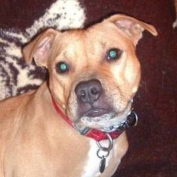
A    X                        B    X
                                      Y                             {Ys }Ss=1         Y
                            θ                            θ

Figure 5: Graphical models under consideration. A The generative model for standard supervised
learning with no data curation. B The generative model with data curation. (Adapted with permission
from Aitchison, 2021).

                                                                     1.05
                                                          Class 0
                                                          Class 1    0.90

                                                                     0.75

                                                                     0.60

                                                                     0.45

                                                                     0.30

                                                                     0.15

                                                                     0.00

Figure 6: A visualisation of P (Y =Undef|X, θ) for toy data (red and blue points) for a network
trained without inputs with undefined class-labels.

from the dataset. In short, the final label Y is chosen to be Y1 if consensus was reached and Undef
otherwise (Fig. 5B).

                                    S         Y1      if Y1 =Y2 = · · · =YS
                           Y |{Ys }s=1 =                                                         (1)
                                              Undef otherwise
From the equation above, we see that Y ∈ Y ∪ {Undef}, that is, Y could be any element from the
label set Y if annotators come to agreement or Undef if consensus is not reached. Suppose further
that all annotators are IID (in the sense that their probability distribution over labels given an input
image is the same). Then, the probability of Y ∈ Y can be written as
                                            QS                                            S
  P (Y =y|X, θ) = P {Ys =y}Ss=1 |X, θ = s=1 P (Ys =y|X, θ) = P (Ys =y|X, θ) = pSy (X)
                                                                                                     (2)
where we have abbreviated the single-annotator probability as py (X) = P (Ys =y|X, θ). When
consensus is not reached (noconsensus), we have:
                                           X                        X
                P (Y =Undef|X, θ) = 1 −        P (Y =y|X, θ) = 1 −     pSy (X).          (3)
                                              y∈Y                               y∈Y

Notice that the maximum of Eq. (3) is achieved when the predictive distribution is uniform: py =
1/C, ∀y ∈ Y, as can be shown using a Lagrange multiplier γ to capture the normalization constraint,
                                                        P
                             L = 1 − y pSy + γ 1 − y py
                                        P
                                                                                               (4)
                                      ∂L
                                0=        = −SpS−1
                                               y   −γ                                               (5)
                                      ∂py
The value of py with maximal L is independent of y, so py is the same for all y ∈ Y, and we must
therefore have py = 1/C. In addition, the minimum of zero is achieved when one of the C classes
has a probability py (X) = 1. Therefore, an input with high predictive (aleatoric) uncertainty is,
by definition, an input with a high probability of disagreement amongst multiple annotators, which
corresponds to having a UCL.

4   Methods
We are able to form a principled log-likelihood objective by combining Eq. (2) for inputs with a
well-defined class-label and Eq. (3) for UCL inputs. However, this model was initially developed

                                                    6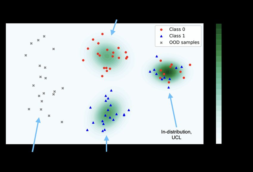
Epoch:0                   Epoch:10                   Epoch:20                  1.0

                                                                                                  0.8

                                                                                                  0.6

                                                                                                  0.4

                                                                                                  0.2

                               Class 0           Class 1       UCL samples                        0.0

Figure 7: A visualisation of the dataset and the experiment results. Samples from the two classes
are represented by red and blue points respectively. Orange points represent synthetic inputs with
undefined class-labels. The colormap shows P (Y =Undef|X, θ), with darker colors indicating more
predictive uncertainty and higher undefined probability.

for cold-posteriors (Aitchison, 2021) and semi-supervised learning (Aitchison, 2020) where the
noconsensus inputs were not known and were omitted from the dataset. In contrast, and following
Hendrycks et al. (2018), we use proxy datasets for UCL inputs, and explicitly maximize the probability
of inputs from those proxy datasets having a UCL (Eq. 7). Importantly, now that we explicitly fit
the probability of an undefined class-label, we need to introduce a little more flexibility into the
model. In particular, a key issue with the current model is that more annotators, S, implies a higher
chance of disagreement hence implying more UCL images. Thus, arbitrary assumptions about the
relative amount of training data with well-defined and undefined class-labels can dramatically affect
our inferences about S. To avoid this, we modify the undefined-class probability by including a
base-rate or bias parameter, c, which modifies the log-odds for well-defined vs undefined class-labels.
In particular, we define the logits to be,

                `0 = c + log 1 − y∈Y pSy (X)                      `y∈Y = log pSy (X)
                                     P
                                                                                                   (6)

where py (X) is the single-annotator probability output by the neural network.
                                          e `0                                             e `y
        P (Y =Undef|X, θ) =               P                     P (Y =y|X, θ) =                           (7)
                                                    e `y
                                                                                           P
                                 e `0 +      y∈Y                                   e`0 +      y∈Y   e`y
with c = 0, this reverts to Eq. (2) and (3), while non-zero c allow us to modify the ratio of well-defined
to undefined class-labels without needing to modify S.
Of course, we do not have the actual datapoints that were rejected during the data curation process,
so instead Dundef is a proxy dataset (e.g. taking CIFAR-10 as Ddef , we might use downsampled
ImageNet with 1000 classes as Dundef ). The objective is,
                 L = EDdef [log P (Y =y|X, θ)] + λEDundef [log P (Y =Undef|X, θ)]                         (8)
where λ represents the relative quantity of inputs with undefined to well-defined class-labels. We use
λ = 1 both for simplicity and because the inclusion of the bias parameter, c, should account for any
mismatch between the “true” and proxy ratios of inputs with well-defined and undefined class-labels.
Finally, in the original formulation of the generative model, S is a fixed, non-negative integer.
However, looking at the actual likelihoods (Eq. 7) there is a straightforward generalisation to real-
valued S ≥ 1. Critically, this allows us to optimize S (and c) using gradient descent to improve
detection of inputs with undefined class-labels even in the absence of changes to the underlying
classifier.

5     Results
5.1   Toy data

First, we conducted an experiment on a toy dataset. We use the make_moons generator from Scikit-
learn (Pedregosa et al., 2011) to generate labelled examples of two classes, with 2000 examples

                                                           7
per class (Fig. 6 and 7). For synthetic UCL points, we use 2000 samples generated from the
make_circles generator (Fig. 7).
We trained a three-layer fully connected neural network with 32 hidden units in each hidden layer for
20 epochs using Adam (Kingma & Ba, 2015) with a constant learning rate of 5 × 10⁻³ . Initially,
we trained without data with undefined class-labels (Fig. 6), and plotted the UCL probability,
P (Y = Undef|X, θ), with high undefined probabilities and uncertain classifications being denoted
by darker colors. This classifier is very certain for all inputs, and therefore judges there to be a
well-defined class-label almost everywhere, except in a small region around the decision boundary. In
contrast, when training with UCL inputs (Fig. 7), the model learns to take points around the training
data as having a well-defined class-label (lighter colors), then classifies points further away as having
UCLs (darker colors). Again, this highlights the difference between OOD and UCL detection: the
region that our model judges as having well-defined class labels covers the training data, but also
extends considerably beyond the training data to regions that could be judged as OOD.
5.2 Image classification
Following our observation in Related Work that some previous OOD detection methods are perhaps
more closely linked to UCL detection, our large-scale experiments are all based on the code from
Hendrycks et al. (2018)2 . We modify these as little as possible, and use the code provided directly as
a baseline for our method. We used an internal cluster of V100 GPUs.
Datasets We were unable to directly replicate the experiments in Hendrycks et al. (2018) because
the requisite datasets are no longer available. In particular, they make heavy use of the 80 million tiny
images dataset (Torralba et al., 2008), which was later withdrawn3 due to the presence of offensive
images and the use of derogatory terms as categories (Prabhu & Birhane, 2020). We are instead
forced to use downsampled ImageNet as Dundef , and we use CIFAR-10, CIFAR-100 and SVHN
as Ddef . Further details on these datasets are given below. CIFAR (Krizhevsky et al., 2009) is a
dataset for natural image classification. CIFAR is made up of CIFAR-10 and CIFAR-100, the former
contains 10 classes while the later contains 100 classes. Both CIFAR-10 and CIFAR-100 have 50k
training samples and 10k test samples. SVHN (Netzer et al., 2011) is a dataset that contains 32x32
colour images of house numbers with ten classes corresponding to digits 0-9. The dataset contains
60k training samples and 26k test samples (note that we did not use the additional 531k samples).
The Downsampled ImageNet dataset introduced by Oord et al. (2016) is a downsampled version of
ImageNet (Deng et al., 2009a)4 with the labels removed. The dataset is designed for unsupervised
learning tasks such as density estimation and image generation.
Test datasets with undefined class-labels At test time, to evaluate our model’s generalisation
power to unseen UCL inputs, we use several types of data originally proposed in Hendrycks &
Gimpel (2016) (as implemented by Hendrycks et al., 2018):
1. Isotropic zero-mean Gaussian noise with σ = 0.5
2. Rademacher noise where each dimension is −1 or 1 with equal probability.
3. Blobs data of algorithmically generated amorphous shapes with definite edges
4. Texture data (Cimpoi et al., 2014) of textural images in the wild.
In addition, the unused training dataset would also be applied for testing. In particular, if ImageNet
was used as Dundef , we would additionally use SVHN for testing. In the case that SVHN is Ddef , we
additionally use CIFAR-10 and CIFAR-100 for testing.
Evaluation metrics UCL detection is in essence a binary classification problem where we treat
UCL inputs as the positive class. It is therefore sensible to use metrics for binary classification to
evaluate a model’s ability to detect inputs with a UCL. While our method gives UCL probabilities,
allowing us to use metrics such as test-log-likelihood and classification error, past work on this topic
does not. As such, to allow for comparison to past work we use three metrics. First, the false positive
rate at N % true positive rate (FPRN ) computes the probability of an input being misclassified as
2
https://github.com/hendrycks/outlier-exposure; Apache 2.0 Licensed
3
groups.csail.mit.edu/vision/TinyImages/
4
access governed agreement at image-net.org/download.php; underlying images are not owned by
ImageNet and have a mixture of licenses
8Dataset FPR95 ↓ AUROC ↑
Ddef Dundef Ours Baseline Ours Baseline
CIFAR-10 ImageNet 21.23 ± 2.73 26.77 ± 1.01 94.49 ± 0.69 92.00 ± 0.40
CIFAR-100 ImageNet 43.33 ± 0.06 52.54 ± 1.12 83.44 ± 0.67 81.10 ± 0.05
SVHN ImageNet 0.51 ± 0.18 1.18 ± 0.28 99.79 ± 0.06 99.72 ± 0.06
Detection Error ↓ AUPR ↑
CIFAR-10 ImageNet 13.23 ± 1.53 23.03 ± 0.83 92.63 ± 0.83 65.40 ± 2.31
CIFAR-100 ImageNet 36.63 ± 1.41 44.52 ± 0.05 50.53 ± 2.28 46.99 ± 0.13
SVHN ImageNet 0.81 ± 0.16 1.51 ± 0.28 99.49 ± 0.11 99.05 ± 0.21
Table 1: Experimental results on a range of different datasets for FPR95, AUROC, Detection Error
and AUPR. Note the arrows indicate the “better” direction (e.g. so lower FPR95 is better). “ImageNet”
refers to Downsampled ImageNet. (The results reported are mean and standard error computed over
5 runs of different random seeds.)
having an undefined class-label (false positive) when at least N % of the true inputs with undefined
class-labels are correctly detected (true positive). In practice, we would like to have a model with low
FPRN % since an ideal model should detect nearly all inputs with undefined class-labels while raising
as few false alarms as possible. Second, the area under the receiver operating characteristic curve
(AUROC) indicates how well the model can discriminate between positive and negative classes, for
example, a model with AUROC of 0.9 would assign a higher probability to an input with undefined
class-label than one with a well-defined class-label 90% of the time. A perfect model would have
an AUROC of 1.0 while an uninformative model with random outputs would have an AUROC of
0.5. Thrid, Detection Error Pe computes the misclassification probability when TPR is 95%. To be
more specific, denote the ratio of positive samples in the test set by ρ, the detection error can be
computed by Pe = (1 − ρ)(1 − TPR) + ρ FPR. Lastly, area under the precision-recall curve (AUPR)
is particularly useful when there exists class imbalance in the dataset: When the number of negative
samples exceeds the number of positive numbers, an increase in the false positive samples would
cause little changes in AUROC, whereas AUPR takes precision into account, which compares false
positives to true positives rather than true negatives, making it suitable for the case where we only
have few true positive samples. A perfect classifier, similar to AUROC, should have an AUPR of 1.0
while a random classifier would have an AUPR identical to the proportion of true positives.
Networks and training protocols The networks and training protocols were chosen to be identical
for our model and the baseline model (Hendrycks et al., 2018) and were implemented directly using
code from Hendrycks et al. (2018). The entire setup and hyperparmeter choices were exactly as in
Hendrycks et al. (2018), so there was very limited scope to alter the experimental setup to favour
our model. Following Hendrycks et al. (2018), the network architecture is chosen to be a 40-2 Wide
Residual Network (Zagoruyko & Komodakis, 2016). Again, following Hendrycks et al. (2018) for
experiments that use SVHN as Ddef , the network is trained for 50 epochs using SGD with an initial
learning rate of 0.01 and for experiments that use CIFAR as Ddef , the network is trained for 100
epochs with an initial learning rate of 0.1. The learning rate in all experiments decays following the
cosine learning rate schedule (Loshchilov & Hutter, 2016). At each iteration, we feed the network
with a mini-batch made up of 128 samples from Ddef and 256 samples from Dundef such that Dundef
will not usually be entirely traversed during a training epoch. For our experiments, we train our model
via maximising the objective in Eq. 8 where c and S are optimised jointly with the parameters of the
network using backpropagation.
Results Broadly, we found that our approach gave superior performance to the baseline (Hendrycks
et al., 2018) using non-probabilistic metrics such as FPR95, AUROC, detection error and AUPR
(Table 1).
6 Conclusion
We establish a new problem: that of UCL detection, and outline how it differs from OOD detection.
We established that certain past methods (e.g. Hendrycks et al., 2018) are perhaps more closely
9related to UCL detection than OOD detection. We develop a new method for UCL detection, which is
based on maximum likelihood in a principled generative model of data curation originally developed
for explaining the cold-posterior effect (Aitchison, 2021). This method gives superior performance to
past methods (Hendrycks et al., 2018) that cannot be written as maximum likelihood inference in a
principle generative model. There are no anticipated social impacts as the work is largely theoretical.
10References
Ahuja, K., Shanmugam, K., Varshney, K., and Dhurandhar, A. Invariant risk minimization games. In
International Conference on Machine Learning, pp. 145–155. PMLR, 2020.
Aitchison, L. A statistical theory of semi-supervised learning. arXiv preprint arXiv:2008.05913,
2020.
Aitchison, L. A statistical theory of cold posteriors in deep neural networks. In International
Conference on Learning Representations, 2021. URL https://openreview.net/forum?id=
Rd138pWXMvG.
Arjovsky, M., Bottou, L., Gulrajani, I., and Lopez-Paz, D. Invariant risk minimization. arXiv preprint
arXiv:1907.02893, 2019.
Bartlett, P. L. and Wegkamp, M. H. Classification with a reject option using a hinge loss. Journal of
Machine Learning Research, 9(8), 2008.
Bendale, A. and Boult, T. E. Towards open set deep networks. In Proceedings of the IEEE conference
on computer vision and pattern recognition, pp. 1563–1572, 2016.
Choi, H., Jang, E., and Alemi, A. A. Waic, but why? generative ensembles for robust anomaly
detection. arXiv preprint arXiv:1810.01392, 2018.
Cimpoi, M., Maji, S., Kokkinos, I., Mohamed, S., , and Vedaldi, A. Describing textures in the wild.
In Proceedings of the IEEE Conf. on Computer Vision and Pattern Recognition (CVPR), 2014.
Cohen, G., Afshar, S., Tapson, J., and Van Schaik, A. Emnist: Extending mnist to handwritten letters.
In 2017 International Joint Conference on Neural Networks (IJCNN), pp. 2921–2926. IEEE, 2017.
Cortes, C., DeSalvo, G., and Mohri, M. Learning with rejection. In International Conference on
Algorithmic Learning Theory, pp. 67–82. Springer, 2016.
Deng, J., Dong, W., Socher, R., Li, L.-J., Li, K., and Fei-Fei, L. Imagenet: A large-scale hierarchical
image database. In 2009 IEEE conference on computer vision and pattern recognition, pp. 248–255.
Ieee, 2009a.
Deng, J., Dong, W., Socher, R., Li, L.-J., Li, K., and Fei-Fei, L. ImageNet: A Large-Scale Hierarchical
Image Database. In CVPR09, 2009b.
DeVries, T. and Taylor, G. W. Learning confidence for out-of-distribution detection in neural networks.
arXiv preprint arXiv:1802.04865, 2018.
Dhamija, A. R., Günther, M., and Boult, T. E. Reducing network agnostophobia. arXiv preprint
arXiv:1811.04110, 2018.
Guénais, T., Vamvourellis, D., Yacoby, Y., Doshi-Velez, F., and Pan, W. Bacoun: Bayesian classifers
with out-of-distribution uncertainty. arXiv preprint arXiv:2007.06096, 2020.
Hendrycks, D. and Gimpel, K. A baseline for detecting misclassified and out-of-distribution examples
in neural networks. arXiv preprint arXiv:1610.02136, 2016.
Hendrycks, D., Mazeika, M., and Dietterich, T. Deep anomaly detection with outlier exposure. In
International Conference on Learning Representations, 2018.
Herbei, R. and Wegkamp, M. H. Classification with reject option. The Canadian Journal of
Statistics/La Revue Canadienne de Statistique, pp. 709–721, 2006.
Kendall, A. and Gal, Y. What uncertainties do we need in bayesian deep learning for computer
vision? arXiv preprint arXiv:1703.04977, 2017.
Kingma, D. P. and Ba, J. Adam: A method for stochastic optimization. In International Conference
on Learning Representations, 2015.
Krizhevsky, A., Hinton, G., et al. Learning multiple layers of features from tiny images. Tech. report,
2009.
11Krueger, D., Caballero, E., Jacobsen, J.-H., Zhang, A., Binas, J., Zhang, D., Priol, R. L., and Courville,
A. Out-of-distribution generalization via risk extrapolation (rex). arXiv preprint arXiv:2003.00688,
2020.
Lakshminarayanan, B., Pritzel, A., and Blundell, C. Simple and scalable predictive uncertainty
estimation using deep ensembles. arXiv preprint arXiv:1612.01474, 2016.
LeCun, Y., Bottou, L., Bengio, Y., and Haffner, P. Gradient-based learning applied to document
recognition. Proceedings of the IEEE, 86(11):2278–2324, 1998.
Lee, K., Lee, H., Lee, K., and Shin, J. Training confidence-calibrated classifiers for detecting
out-of-distribution samples. arXiv preprint arXiv:1711.09325, 2017.
Liang, S., Li, Y., and Srikant, R. Principled detection of out-of-distribution examples in neural
networks. arXiv preprint arXiv:1706.02690, pp. 655–662, 2017.
Liu, S., Garrepalli, R., Dietterich, T., Fern, A., and Hendrycks, D. Open category detection with pac
guarantees. In International Conference on Machine Learning, pp. 3169–3178. PMLR, 2018.
Loshchilov, I. and Hutter, F. Sgdr: Stochastic gradient descent with warm restarts. arXiv preprint
arXiv:1608.03983, 2016.
Milios, D., Michiardi, P., and Filippone, M. A variational view on bootstrap ensembles as bayesian
inference. arXiv preprint arXiv:2006.04548, 2020.
Morningstar, W. R., Ham, C., Gallagher, A. G., Lakshminarayanan, B., Alemi, A. A., and Dillon, J. V.
Density of states estimation for out-of-distribution detection. arXiv preprint arXiv:2006.09273,
2020.
Mozannar, H. and Sontag, D. Consistent estimators for learning to defer to an expert. In International
Conference on Machine Learning, pp. 7076–7087. PMLR, 2020.
Mu, N. and Gilmer, J. Mnist-c: A robustness benchmark for computer vision. arXiv preprint
arXiv:1906.02337, 2019.
Nalisnick, E., Matsukawa, A., Teh, Y. W., Gorur, D., and Lakshminarayanan, B. Do deep generative
models know what they don’t know? arXiv preprint arXiv:1810.09136, 2018.
Netzer, Y., Wang, T., Coates, A., Bissacco, A., Wu, B., and Ng, A. Reading digits in natural images
with unsupervised feature learning. Feature Learning NIPS Workshop on Deep Learning and
Unsupervised Feature Learning, 2011.
Oord, A., Kalchbrenner, N., and Kavukcuoglu, K. Pixel recurrent neural networks. ArXiv,
abs/1601.06759, 2016.
Pearce, T., Zaki, M., and Neely, A. Bayesian neural network ensembles. arXiv preprint
arXiv:1811.12188, 2018.
Pedregosa, F., Varoquaux, G., Gramfort, A., Michel, V., Thirion, B., Grisel, O., Blondel, M.,
Prettenhofer, P., Weiss, R., Dubourg, V., Vanderplas, J., Passos, A., Cournapeau, D., Brucher, M.,
Perrot, M., and Duchesnay, E. Scikit-learn: Machine learning in Python. Journal of Machine
Learning Research, 12:2825–2830, 2011.
Pidhorskyi, S., Almohsen, R., Adjeroh, D. A., and Doretto, G. Generative probabilistic novelty
detection with adversarial autoencoders. arXiv preprint arXiv:1807.02588, 2018.
Prabhu, V. U. and Birhane, A. Large image datasets: A pyrrhic win for computer vision? arXiv
preprint arXiv:2006.16923, 2020.
Ren, J., Liu, P. J., Fertig, E., Snoek, J., Poplin, R., DePristo, M. A., Dillon, J. V., and Lakshmi-
narayanan, B. Likelihood ratios for out-of-distribution detection. arXiv preprint arXiv:1906.02845,
2019.
Scheirer, W. J., de Rezende Rocha, A., Sapkota, A., and Boult, T. E. Toward open set recognition.
IEEE transactions on pattern analysis and machine intelligence, 35(7):1757–1772, 2012.
12Scheirer, W. J., Jain, L. P., and Boult, T. E. Probability models for open set recognition. IEEE
transactions on pattern analysis and machine intelligence, 36(11):2317–2324, 2014.
Shafaei, A., Schmidt, M., and Little, J. J. Does your model know the digit 6 is not a cat? a less biased
evaluation of" outlier" detectors. CoRR, 2018.
Torralba, A., Fergus, R., and Freeman, W. T. 80 million tiny images: A large data set for nonparametric
object and scene recognition. IEEE transactions on pattern analysis and machine intelligence, 30
(11):1958–1970, 2008.
Vernekar, S., Gaurav, A., Abdelzad, V., Denouden, T., Salay, R., and Czarnecki, K. Out-of-distribution
detection in classifiers via generation. arXiv preprint arXiv:1910.04241, 2019.
Wang, W., Wang, A., Tamar, A., Chen, X., and Abbeel, P. Safer classification by synthesis. arXiv
preprint arXiv:1711.08534, 2017.
Zagoruyko, S. and Komodakis, N. Wide residual networks. In BMVC, 2016.
Checklist
1. For all authors...
(a) Do the main claims made in the abstract and introduction accurately reflect the paper’s
contributions and scope? [Yes]
(b) Did you describe the limitations of your work? [Yes] (Though none are anticipated)
(c) Did you discuss any potential negative societal impacts of your work? [Yes]
(d) Have you read the ethics review guidelines and ensured that your paper conforms to
them? [Yes]
2. If you are including theoretical results...
(a) Did you state the full set of assumptions of all theoretical results? [Yes]
(b) Did you include complete proofs of all theoretical results? [Yes]
3. If you ran experiments...
(a) Did you include the code, data, and instructions needed to reproduce the main experi-
mental results (either in the supplemental material or as a URL)? [Yes]
(b) Did you specify all the training details (e.g., data splits, hyperparameters, how they
were chosen)? [Yes]
(c) Did you report error bars (e.g., with respect to the random seed after running experi-
ments multiple times)? [Yes]
(d) Did you include the total amount of compute and the type of resources used (e.g., type
of GPUs, internal cluster, or cloud provider)? [Yes] Included in the README.md in
the code repo
4. If you are using existing assets (e.g., code, data, models) or curating/releasing new assets...
(a) If your work uses existing assets, did you cite the creators? [Yes]
(b) Did you mention the license of the assets? [Yes] (where license clear)
(c) Did you include any new assets either in the supplemental material or as a URL? [Yes]
Code at anonymous.4open.science/r/58f3/
(d) Did you discuss whether and how consent was obtained from people whose data you’re
using/curating? [N/A] Standard datasets
(e) Did you discuss whether the data you are using/curating contains personally identifiable
information or offensive content? [N/A] Standard datasets
13You can also read