Attention Guided Anomaly Localization in Images
←
→
Page content transcription
If your browser does not render page correctly, please read the page content below

Attention Guided Anomaly Localization in
                                                                 Images

                                                   Shashanka Venkataramanan?[0000−0003−1096−1342] , Kuan-Chuan
                                                    †[0000−0002−2682−9912]
                                              Peng                   , Rajat Vikram Singh‡[0000−0002−1416−8344] , and
                                                            Abhijit Mahalanobis?[0000−0002−2782−8655]
                                         ?
                                             Center for Research in Computer Vision, University of Central Florida, Orlando, FL
arXiv:1911.08616v4 [cs.CV] 17 Jul 2020

                                                        †
                                                          Mitsubishi Electric Research Laboratories, Cambridge, MA
                                                               ‡
                                                                 Siemens Corporate Technology, Princeton, NJ
                                               shashankv@Knights.ucf.edu, kpeng@merl.com, singh.rajat@siemens.com,
                                                                           amahalan@crcv.ucf.edu

                                                  Abstract. Anomaly localization is an important problem in computer
                                                  vision which involves localizing anomalous regions within images with
                                                  applications in industrial inspection, surveillance, and medical imaging.
                                                  This task is challenging due to the small sample size and pixel coverage of
                                                  the anomaly in real-world scenarios. Most prior works need to use anoma-
                                                  lous training images to compute a class-specific threshold to localize
                                                  anomalies. Without the need of anomalous training images, we propose
                                                  Convolutional Adversarial Variational autoencoder with Guided Atten-
                                                  tion (CAVGA), which localizes the anomaly with a convolutional latent
                                                  variable to preserve the spatial information. In the unsupervised setting,
                                                  we propose an attention expansion loss where we encourage CAVGA to
                                                  focus on all normal regions in the image. Furthermore, in the weakly-
                                                  supervised setting we propose a complementary guided attention loss,
                                                  where we encourage the attention map to focus on all normal regions
                                                  while minimizing the attention map corresponding to anomalous regions
                                                  in the image. CAVGA outperforms the state-of-the-art (SOTA) anomaly
                                                  localization methods on MVTec Anomaly Detection (MVTAD), modified
                                                  ShanghaiTech Campus (mSTC) and Large-scale Attention based Glau-
                                                  coma (LAG) datasets in the unsupervised setting and when using only
                                                  2% anomalous images in the weakly-supervised setting. CAVGA also out-
                                                  performs SOTA anomaly detection methods on the MNIST, CIFAR-10,
                                                  Fashion-MNIST, MVTAD, mSTC and LAG datasets.

                                                  Keywords: guided attention, anomaly localization, convolutional ad-
                                                  versarial variational autoencoder

                                         1      Introduction
                                         Recognizing whether an image is homogeneous with its previously observed dis-
                                         tribution or whether it belongs to a novel or anomalous distribution has been
                                         identified as an important problem [5]. In this work, we focus on a related task,
                                         anomaly localization in images, which involves segmenting the anomalous regions
2       S. Venkataramanan et al.

                                                       dataset    task   improvement
                                                     MVTAD [5]      l (9/15; 4∼85%)
                                                     MVTAD [5]      d (9/15; 2∼30%)
                                                     mSTC [31]      l (7/12; 2∼42%)
                                                     mSTC [31]      d (8/12; 1∼38%)
                                                      LAG [29]      l    (1/1; 16%)
                                                      LAG [29]      d    (1/1; 1.1%)
                                                     MNIST [27]     d (8/10; 0.1∼2.5%)
                                                    CIFAR-10 [25]   d (7/10; 3∼31%)
                                                    F-MNIST [57]    d (8/10; 2∼24%)

                                                        l: localization; d: detection
                                                      F-MNIST: Fashion-MNIST [57]

                                                     • metric for l : IoU
                                                     • metric for d in MVTAD, mSTC,
                                                     and LAG: classification accuracy
                                                     • metric for d in MNIST,
                                                     CIFAR-10 and Fashion-MNIST:
                                                     area under ROC curve

              (i) CAVGA main idea                     (ii) improvement summary

Fig. 1: (i) CAVGA uses the proposed complementary guided attention loss to
encourage the attention map to cover the entire normal regions while suppressing
the attention map corresponding to anomalous class in the training image. This
enables the trained network to generate the anomalous attention map to localize
the anomaly better at testing (ii) CAVGA’s improvement over SOTA in the form
of (number of outperforming/total categories; improvement (%) in its metric)

within them. Anomaly localization has been applied in industrial inspection set-
tings to segment defective product parts [5], in surveillance to locate intruders
[38], in medical imaging to segment tumor in brain MRI or glaucoma in retina
images [4, 29], etc. There has been an increase in analysis towards segmenting
potential anomalous regions in images as acknowledged in [13].
    Existing state-of-the-art (SOTA) anomaly localization methods [6, 47] are
based on deep learning. However, developing deep learning based algorithms for
this task can be challenging due to the small pixel coverage of the anomaly and
lack of suitable data since images with anomalies are rarely available in real-world
scenarios [5]. Existing SOTA methods tackle this challenge using autoencoders
[15, 47] and GAN based approaches [3, 43, 59], which use a thresholded pixel-
wise difference between the input and reconstructed image to localize anomalies.
But, their methods need to determine class-specific thresholds using anomalous
training images which can be unavailable in real-world scenarios.
    To tackle these drawbacks of using anomalous training images, we propose
Convolutional Adversarial Variational autoencoder with Guided Attention
(CAVGA), an unsupervised anomaly localization method which requires no
anomalous training images. CAVGA comprises of a convolutional latent vari-
able to preserve the spatial relation between the input and latent variable. Since
real-world applications may have access to only limited training data [5], we
propose to localize the anomalies by using supervision on attention maps. This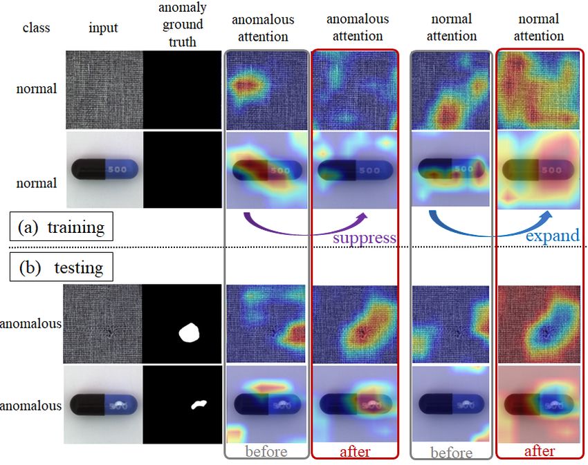
Attention Guided Anomaly Localization in Images        3

is motivated by the finding in [28] that attention based supervision can alleviate
the need of using large amount of training data. Intuitively, without any prior
knowledge of the anomaly, humans need to look at the entire image to identify
the anomalous regions. Based on this idea, we propose an attention expansion
loss where we encourage the network to generate an attention map that focuses
on all normal regions of the image.
    Since annotating segmentation training data can be laborious [22], in the
case when the annotator provides few anomalous training images without ground
truth segmented anomalous regions, we extend CAVGA to a weakly supervised
setting. Here, we introduce a classifier in CAVGA and propose a complementary
guided attention loss computed only for the normal images correctly predicted
by the classifier. Using this complementary guided attention loss, we expand the
normal attention but suppress the anomalous attention on the normal image,
where normal/anomalous attention represents the areas affecting the classifier’s
normal/anomalous prediction identified by existing network visualization meth-
ods (e.g. Grad-CAM [49]). Fig. 1 (i) (a) illustrates our attention mechanism
during training, and Fig. 1 (i) (b) demonstrates that the resulting normal at-
tention and anomalous attention on the anomalous testing images are visually
complementary, which is consistent with our intuition. Furthermore, Fig. 1 (ii)
summarizes CAVGA’s ability to outperform SOTA methods in anomaly local-
ization on industrial inspection (MVTAD) [5], surveillance (mSTC) [31] and
medical imaging (LAG) [29] datasets. We also show CAVGA’s ability to outper-
form SOTA methods in anomaly detection on common benchmarks.
    To the best of our knowledge, we are the first in anomaly localization to
propose an end-to-end trainable framework with attention guidance which ex-
plicitly enforces the network to learn representations from the entire normal
image. As compared to the prior works, our proposed approach CAVGA needs
no anomalous training images to determine a class-specific threshold to localize
the anomaly. Our contributions are:
 – An attention expansion loss (Lae ), where we encourage the network to
   focus on the entire normal images in the unsupervised setting.
 – A complementary guided attention loss (Lcga ), which we use to mini-
   mize the anomalous attention and simultaneously expand the normal atten-
   tion for the normal images correctly predicted by the classifier.
 – New SOTA: In anomaly localization, CAVGA outperforms SOTA methods
   on the MVTAD and mSTC datasets in IoU and mean Area under ROC
   curve (AuROC) and also outperforms SOTA anomaly localization methods
   on LAG dataset in IoU. We also show CAVGA’s ability to outperform SOTA
   methods for anomaly detection on the MVTAD, mSTC, LAG, MNIST [27],
   CIFAR-10 [25] and Fashion-MNIST [57] datasets in classification accuracy.

2   Related Works
Often used interchangeably, the terms anomaly localization and anomaly seg-
mentation involve pixel-accurate segmentation of anomalous regions within an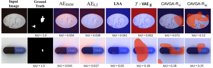
4       S. Venkataramanan et al.

Table 1: Comparison between CAVGA and other anomaly localization methods
in the unsupervised setting in terms of the working properties. Among all the
listed methods, only CAVGA satisfies all the listed properties
      Does the method satisfy each property?   [3, 48]   [4]   [47]   [54]   [13, 32]   CAVGA
                                               [6, 43]                [50]      [2]
       not using anomalous training images       N       N     Y      Y        Y         Y
       localize multiple modes of anomalies      Y       N     N      N        Y         Y
        pixel (not patch) based localization     Y       Y     N      Y        Y         Y
        use convolutional latent variable        N       Y     N      N        N         Y

image [5]. They have been applied to industrial inspection settings to segment
defective product parts [5], medical imaging to segment glaucoma in retina im-
ages [29], etc. Image based anomaly localization has not been fully studied as
compared to anomaly detection, where methods such as [3, 4, 6, 43, 48] employ
a thresholded pixel wise difference between the input and reconstructed image
to segment the anomalous regions. [47] proposes an inpainter-detector network
for patch-based localization in images. [13] proposes gradient descent on a regu-
larized autoencoder while Liu et al. [32] (denoted as ADVAE) generate gradient
based attention maps from the latent space of the trained model. We compare
CAVGA with the existing methods relevant to anomaly localization in the un-
supervised setting in Table 1 and show that among the listed methods, only
CAVGA shows all the listed properties.
    Anomaly detection involves determining an image as normal or anomalous
[3]. One-class classification and anomaly detection are related to novelty detec-
tion [41] which has been widely studied in computer vision [3, 20, 35, 37, 53]
and applied to video analysis [10], remote sensing [36], etc. With the advance in
GANs [17], SOTA methods perform anomaly detection by generating realistic
normal images during training [21, 22, 42, 46, 48]. [12] proposes to search the la-
tent space of the generator for detecting anomalies. [41] introduces latent-space-
sampling-based network with information-negative mining while [30] proposes
normality score function based on capsule network’s activation and reconstruc-
tion error. [2] proposes a deep autoencoder that learns the distribution of latent
representation through autoregressive procedure. Unlike [7, 11, 44, 55] where
anomalous training images are used for anomaly detection, CAVGA does not
need anomalous training images.

3     Proposed Approach: CAVGA

3.1   Unsupervised Approach: CAVGAu

Fig. 2 (a) illustrates CAVGA in the unsupervised setting (denoted as CAVGAu ).
CAVGAu comprises of a convolutional latent variable to preserve the spatial
information between the input and latent variable. Since attention maps obtained
from feature maps illustrate the regions of the image responsible for specific
Attention Guided Anomaly Localization in Images           5

Fig. 2: (a) The framework of CAVGAu where the attention expansion loss Lae
guides the attention map A computed from the latent variable z to cover the en-
tire normal image. (b) Illustration of CAVGAw with the complementary guided
attention loss Lcga to minimize the anomalous attention Acxa and expand the
normal attention Acxn for the normal images correctly predicted by the classifier

activation of neurons in the feature maps [58], we propose an attention expansion
loss such that the feature representation of the latent variable encodes all the
normal regions. This loss encourages the attention map generated from the latent
variable to cover the entire normal training image as illustrated in Fig. 1 (i) (a).
During testing, we localize the anomaly from the areas of the image that the
attention map does not focus on.
    Convolutional latent variable Variational Autoencoder (VAE) [23] is a
generative model widely used for anomaly detection [24, 40]. The loss function
of training a vanilla VAE can be formulated as:
                      L = LR (x, x̂) + KL(qφ (z|x)||pθ (z|x)),                     (1)
                      PN
where LR (x, x̂) = −1
                   N    i=1 xi log(x̂i )+(1−xi )log(1−x̂i ) is the reconstruction loss
between the input (x) and reconstructed images (x̂), and N is the total number of
images. The posterior pθ (z|x) is modeled using a standard Gaussian distribution
prior p(z) with the help of Kullback-Liebler (KL) divergence through qφ (z|x).
Since the vanilla VAE results in blurry reconstruction [26], we use a discriminator
(D(.)) to improve the stability of the training and generate sharper reconstructed
images x̂ using adversarial learning [34] formulated as follows:
                                N
                             1 X
                  Ladv = −         log(D(xi )) + log(1 − D(x̂i ))                 (2)
                             N i=1
6 S. Venkataramanan et al.
Unlike traditional autoencoders [6, 18] where the latent variable is flattened,
inspired from [4], we use a convolutional latent variable to preserve the spatial
relation between the input and the latent variable.
Attention expansion loss Lae The main contribution of our work involves
using supervision on attention maps to spatially localize the anomaly in the im-
age. Most methods [3, 48, 53] employ a thresholded pixel-wise difference between
the reconstructed image and the input image to localize the anomaly where the
threshold is determined by using anomalous training images. However, CAVGAu
learns to localize the anomaly using an attention map reflected through an end-
to-end training process without the need of any anomalous training images. We
use the feature representation of the latent variable z to compute the attention
map (A). A is computed using Grad-CAM [49] such that Ai,j ∈ [0, 1], where Ai,j
is the (i, j) element of A.
Intuitively, A obtained from feature maps focuses on the regions of the im-
age based on the activation of neurons in the feature maps and its respective
importance [58, 60]. Due to the lack of prior knowledge about the anomaly, in
general, humans need to look at the entire image to identify anomalous regions.
We use this notion to learn the feature representation of the entire normal im-
age by proposing an attention expansion loss, where we encourage the network
to generate an attention map covering all the normal regions. This attention
expansion loss for each image Lae,1 is defined as:
1 X
Lae,1 = (1 − Ai,j ) (3)
|A| i,j
where |A| is the total number of elements in A. The final attention expansion
loss Lae is the average of Lae,1 over the N images. Since the idea of attention
mechanisms involves locating the most salient regions in the image [29] which
typically does not cover the entire image, we use Lae as an additional supervision
on the network, such that the trained network generates an attention map that
covers all the normal regions. Fig. 1 (i) (a) shows that before using Lae i.e. train-
ing CAVGAu only with adversarial learning (Ladv + L) does not encode all the
normal regions into the latent variable, and that the attention map fails to cover
the entire image, which is overcome after using Lae . Furthermore, supervising
on attention maps prevents the trained model to make inference based on incor-
rect areas and also alleviates the need of using large amount of training data as
shown in [28], which is not explicitly enforced in existing methods [3, 6, 47].
We form the final objective function Lf inal below:
Lf inal = wr L + wadv Ladv + wae Lae , (4)
where wr , wadv , and wae are empirically set as 1, 1, and 0.01 respectively.
During testing, we feed an image xtest into the encoder followed by the de-
coder, which reconstructs an image x̂test . As defined in [48], we compute the
pixel-wise difference between x̂test and xtest as the anomalous score sa . Intu-
itively, if xtest is drawn from the learnt distribution of z, then sa is small. WithoutAttention Guided Anomaly Localization in Images 7
using any anomalous training images in the unsupervised setting, we normalize
sa between [0, 1] and empirically set 0.5 as the threshold to detect an image as
anomalous. The attention map Atest is computed from z using Grad-CAM and
is inverted (1 - Atest ) to obtain an anomalous attention map which localizes the
anomaly. Here, 1 refers to a matrix of all ones with the same dimensions as Atest .
We empirically choose 0.5 as the threshold on the anomalous attention map to
evaluate the localization performance.
3.2 Weakly Supervised Approach: CAVGAw
CAVGAu can be further extended to a weakly supervised setting (denoted as
CAVGAw ) where we explore the possibility of using few anomalous training
images to improve the performance of anomaly localization. Given the labels
of the anomalous and normal images without the pixel-wise annotation of the
anomaly during training, we modify CAVGAu by introducing a binary classifier
C at the output of z as shown in Fig. 2 (b) and train C using the binary cross
entropy loss Lbce . Given an image x and its ground truth label y, we define
p ∈ {ca , cn } as the prediction of C, where ca and cn are anomalous and normal
classes respectively. From Fig. 2 (b) we clone z into a new tensor, flatten it to
form a fully connected layer zf c , and add a 2-node output layer to form C. z
and zf c share parameters. Flattening zf c enables a higher magnitude of gradient
backpropagation from p [49].
Complementary guided attention loss Lcga Although, attention maps
generated from a trained classifier have been used in weakly supervised semantic
segmentation tasks [39, 49], to the best of our knowledge, we are the first to
propose supervision on attention maps for anomaly localization in the weakly
supervised setting. Since the attention map depends on the performance of C
[28], we propose the complementary guided attention loss Lcga based on C’s
prediction to improve anomaly localization. We use Grad-CAM to compute the
attention map for the anomalous class Acxa and the attention map for the normal
class Acxn on the normal image x (y = cn ). Using Acxa and Acxn , we propose
Lcga where we minimize the areas covered by Acxa but simultaneously enforce
Acxn to cover the entire normal image. Since the attention map is computed
by backpropagating the gradients from p, any incorrect p would generate an
undesired attention map. This would lead to the network learning to focus on
erroneous areas of the image during training, which we avoid using Lcga . We
compute Lcga only for the normal images correctly classified by the classifier i.e.
if p = y = cn . We define Lcga,1 , the complementary guided attention loss for
each image, in the weakly supervised setting as:
1 (p = y = cn ) X
Lcga,1 = (1 − (Acxn )i,j + (Acxa )i,j ), (5)
|Acxn | i,j
where 1 (·) is an indicator function. Lcga is the average of Lcga,1 over the N
images. Our final objective function Lf inal is defined as:
Lf inal = wr L + wadv Ladv + wc Lbce + wcga Lcga , (6)8 S. Venkataramanan et al.
Table 2: Our experimental settings. Notations: u: unsupervised; w: weakly su-
pervised; DM : MNIST [27]; DF : Fashion-MNIST [57]; DC : CIFAR-10 [25]
property \ dataset MVTAD [5] mSTC [31] LAG [29] DM DF DC
setting u w u w u u u u
# total classes 15 15 13 13 1 10 10 10
# normal training images 3629 3629 244875 244875 2632 ∼6k 6k 5k
# anomalous training images 0 35 0 1763 0 0 0 0
# normal testing images 467 467 21147 21147 800 ∼1k 1k 1k
# anomalous testing images 1223 1223 86404 86404 2392 ∼9k 9k 9k
where wr , wadv , wc , and wcga are empirically set as 1, 1, 0.001, and 0.01 respec-
tively. During testing, we use C to predict the input image xtest as anomalous or
normal. The anomalous attention map Atest of xtest is computed when y = ca .
We use the same evaluation method as that in Sec. 3.1 for anomaly localization.
4 Experimental Setup
Benchmark datasets: We evaluate CAVGA on the MVTAD [5], mSTC [31]
and LAG [29] datasets for anomaly localization, and the MVTAD, mSTC, LAG,
MNIST [27], CIFAR-10 [25] and Fashion-MNIST [57] datasets for anomaly de-
tection. Since STC dataset [31] is designed for video instead of image anomaly
detection, we extract every 5th frame of the video from each scene for training
and testing without using any temporal information. We term the modified STC
dataset as mSTC and summarize the experimental settings in Table 2.
Baseline methods: For anomaly localization, we compare CAVGA with
AVID [47], AEL2 [6], AESSIM [6], AnoGAN [48], CNN feature dictionary (CN-
NFD) [37], texture inspection (TI) [8], γ-VAE grad [13] (denoted as γ-VAEg ),
LSA [2], ADVAE [32] and variation model (VM) [52] based approaches on the
MVTAD and mSTC datasets. Since [13] does not provide the code for their
method, we adapt the code from [1] and report its best result using our experi-
mental settings. We also compare CAVGAu with CAM [60], GBP [51], Smooth-
Grad [50] and Patho-GAN [54] on the LAG dataset. In addition, we compare
CAVGAu with LSA [2], OCGAN [41], ULSLM [56], CapsNet PP-based and Cap-
sNet RE-based [30] (denoted as CapsNetPP and CapsNetRE ), AnoGAN [48],
ADGAN [12], and β-VAE [21] on the MNIST, CIFAR-10 and Fashion-MNIST
datasets for anomaly detection.
Architecture details: Based on the framework in Fig. 2 (a), we use the con-
volution layers of ResNet-18 [19] as our encoder pretrained from ImageNet [45]
and finetuned on each category / scene individually. Inspired from [9], we propose
to use the residual generator as our residual decoder by modifying it with a con-
volution layer interleaved between two upsampling layers. The skip connection
added from the output of the upsampling layer to the output of the convolution
layer, increases mutual information between observations and latent variable and
also avoids latent variable collapse [14]. We use the discriminator of DC-GANAttention Guided Anomaly Localization in Images 9
Table 3: Performance comparison of anomaly localization in category-specific
IoU, mean IoU (IoU), and mean AuROC (AuROC) on the MVTAD dataset.
The darker cell color indicates better performance ranking in each row
Category AVID AESSIM AEL2 AnoGAN γ-VAEg LSA ADVAE CAVGA CAVGA CAVGA CAVGA
[47] [6] [6] [48] [13] [2] [32] -Du -Ru -Dw -Rw
Bottle 0.28 0.15 0.22 0.05 0.27 0.27 0.27 0.30 0.34 0.36 0.39
Hazelnut 0.54 0.00 0.41 0.02 0.63 0.41 0.44 0.44 0.51 0.58 0.79
Capsule 0.21 0.09 0.11 0.04 0.24 0.22 0.11 0.25 0.31 0.38 0.41
Metal Nut 0.05 0.01 0.26 0.00 0.22 0.38 0.49 0.39 0.45 0.46 0.46
Leather 0.32 0.34 0.67 0.34 0.41 0.77 0.24 0.76 0.79 0.80 0.84
Pill 0.11 0.07 0.25 0.17 0.48 0.18 0.18 0.34 0.40 0.44 0.53
Wood 0.14 0.36 0.29 0.14 0.45 0.41 0.14 0.56 0.59 0.61 0.66
Carpet 0.25 0.69 0.38 0.34 0.79 0.76 0.10 0.71 0.73 0.70 0.81
Tile 0.09 0.04 0.23 0.08 0.38 0.32 0.23 0.31 0.38 0.47 0.81
Grid 0.51 0.88 0.83 0.04 0.36 0.20 0.02 0.32 0.38 0.42 0.55
Cable 0.27 0.01 0.05 0.01 0.26 0.36 0.18 0.37 0.44 0.49 0.51
Transistor 0.18 0.01 0.22 0.08 0.44 0.21 0.30 0.30 0.35 0.38 0.45
Toothbrush 0.43 0.08 0.51 0.07 0.37 0.48 0.14 0.54 0.57 0.60 0.63
Screw 0.22 0.03 0.34 0.01 0.38 0.38 0.17 0.42 0.48 0.51 0.66
Zipper 0.25 0.10 0.13 0.01 0.17 0.14 0.06 0.20 0.26 0.29 0.31
IoU 0.26 0.19 0.33 0.09 0.39 0.37 0.20 0.41 0.47 0.50 0.59
AuROC 0.78 0.87 0.82 0.74 0.86 0.79 0.86 0.85 0.89 0.92 0.93
[42] pretrained on the Celeb-A dataset [33] and finetuned on our data as our
discriminator and term this network as CAVGA-R. For fair comparisons with
the baseline approaches in terms of network architecture, we use the discrimina-
tor and generator of DC-GAN pretrained on the Celeb-A dataset as our encoder
and decoder respectively. We keep the same discriminator as discussed previously
and term this network as CAVGA-D. CAVGA-Du and CAVGA-Ru are termed
as CAVGAu in the unsupervised setting, and CAVGA-Dw and CAVGA-Rw as
CAVGAw in weakly supervised setting respectively.
Training and evaluation: For anomaly localization and detection on the
MVTAD, mSTC and LAG datasets, the network is trained only on normal im-
ages in the unsupervised setting. In the weakly supervised setting, since none
of the baseline methods provide the number of anomalous training images they
use to compute the threshold, we randomly choose 2% of the anomalous images
along with all the normal training images for training. On the MNIST, CIFAR-
10 and Fashion-MNIST datasets, we follow the same procedure as defined in
[12] (training/testing uses single class as normal and the rest of the classes as
anomalous. We train CAVGA-Du using this normal class). For anomaly localiza-
tion, we show the AuROC [5] and the Intersection-over-Union (IoU) between the
generated attention map and the ground truth. Following [5], we use the mean
of accuracy of correctly classified anomalous images and normal images to eval-
uate the performance of anomaly detection on both the normal and anomalous
images on the MVTAD, mSTC and LAG datasets. On the MNIST, CIFAR-10,
and Fashion-MNIST datasets, same as [12], we use AuROC for evaluation.10 S. Venkataramanan et al.
5 Experimental Results
We use the cell color in the quantitative result tables to denote the performance
ranking in that row, where darker cell color means better performance.
Performance on anomaly localization: Fig. 3 (a) shows the qualitative
results and Table 3 shows that CAVGAu localizes the anomaly better com-
pared to the baselines on the MVTAD dataset. CAVGA-Du outperforms the
best performing baseline method (γ-VAEg ) in mean IoU by 5%. Most baselines
use anomalous training images to compute class-specific threshold to localize
anomalies. Needing no anomalous training images, CAVGA-Du still outperforms
all the mentioned baselines in mean IoU. In terms of mean AuROC, CAVGA-Du
outperforms CNNFD, TI and VM by 9%, 12% and 10% respectively and achieves
comparable results with best baseline method. Table 3 also shows that CAVGA-
Dw outperforms CAVGA-Du by 22% and 8% on mean IoU and mean AuROC
respectively. CAVGA-Dw also outperforms the baselines in mean AuROC. Fig. 4
illustrates that one challenge in anomaly localization is the low contrast between
the anomalous regions and their background. In such scenarios, although still
outperforming the baselines, CAVGA does not localize the anomaly well.
Fig. 3: Qualitative results on (a) MVTAD & (b) mSTC datasets respectively.
The anomalous attention map (in red) depicts the localization of the anomaly
Fig. 3 (b) illustrates the qualitative results and Table 4 shows that CAVGA
also outperforms the baseline methods in mean IoU and mean AuROC on the
mSTC dataset. Table 5 shows that CAVGA outperforms the most competitive
baseline Patho-GAN [54] by 16% in IoU on the LAG dataset. CAVGA is prac-
tically reasonable to train on a single GTX 1080Ti GPU, having comparable
training and testing time with baseline methods.Attention Guided Anomaly Localization in Images 11
Table 4: Performance comparison of anomaly localization in IoU and its mean
(IoU) along with anomaly detection in terms of mean of accuracy of correctly
classified anomalous images and normal images on the mSTC dataset for each
scene ID si . For anomaly localization, we also list the mean AuROC (AuROC)
Task \ Method si γ-VAEg AVID LSA AESSIM AEL2 CAVGA CAVGA CAVGA CAVGA
[13] [47] [2] [6] [6] -Du -Ru -Dw -Rw
01 0.239 0.182 0.244 0.201 0.163 0.267 0.316 0.383 0.441
02 0.206 0.206 0.183 0.081 0.172 0.190 0.234 0.257 0.349
03 0.272 0.162 0.265 0.218 0.240 0.277 0.293 0.313 0.465
04 0.290 0.263 0.271 0.118 0.125 0.283 0.349 0.360 0.381
05 0.318 0.234 0.287 0.162 0.129 0.291 0.312 0.408 0.478
Localization 06 0.337 0.314 0.238 0.215 0.198 0.344 0.420 0.455 0.589
07 0.168 0.214 0.137 0.191 0.165 0.198 0.241 0.284 0.366
08 0.220 0.168 0.233 0.069 0.056 0.219 0.254 0.295 0.371
09 0.174 0.193 0.187 0.038 0.021 0.247 0.284 0.313 0.365
10 0.146 0.137 0.146 0.116 0.141 0.149 0.166 0.245 0.295
11 0.277 0.264 0.286 0.101 0.075 0.309 0.372 0.441 0.588
12 0.162 0.180 0.108 0.203 0.164 0.098 0.141 0.207 0.263
IoU 0.234 0.210 0.215 0.143 0.137 0.239 0.281 0.330 0.412
AuROC 0.82 0.77 0.81 0.76 0.74 0.83 0.85 0.89 0.90
01 0.75 0.68 0.75 0.65 0.72 0.77 0.85 0.84 0.87
02 0.75 0.75 0.79 0.70 0.61 0.76 0.84 0.89 0.90
03 0.81 0.68 0.63 0.79 0.71 0.82 0.84 0.86 0.88
04 0.83 0.71 0.79 0.81 0.66 0.80 0.80 0.81 0.83
05 0.86 0.59 0.68 0.71 0.67 0.81 0.86 0.90 0.94
Detection 06 0.59 0.62 0.58 0.47 0.55 0.64 0.67 0.65 0.70
07 0.59 0.63 0.63 0.36 0.59 0.60 0.64 0.75 0.77
08 0.77 0.73 0.75 0.69 0.70 0.74 0.74 0.76 0.80
09 0.89 0.88 0.79 0.84 0.73 0.87 0.88 0.90 0.91
10 0.64 0.80 0.84 0.83 0.88 0.88 0.92 0.94 0.94
11 0.78 0.68 0.71 0.71 0.75 0.79 0.81 0.83 0.83
12 0.71 0.66 0.63 0.65 0.52 0.76 0.79 0.81 0.83
avg 0.75 0.70 0.71 0.68 0.67 0.77 0.80 0.83 0.85
Table 5: Performance comparison of anomaly localization in IoU along with
anomaly detection in terms of classification accuracy on the LAG dataset [29]
Task \ Method CAM [60] GBP [51] SmoothGrad [50] Patho-GAN [54] CAVGA-Du
Localization 0.13 0.09 0.14 0.37 0.43
Detection 0.68 0.84 0.79 0.89 0.90
Fig. 4: Examples of incorrect localization of the anomaly on the MVTAD dataset
by CAVGA-Ru and CAVGA-Rw12 S. Venkataramanan et al.
Table 6: The mean of accuracy of correctly classified anomalous images and
normal images in anomaly detection on the MVTAD dataset
Category AVID AESSIM AEL2 AnoGAN γ-VAEg LSA CAVGA CAVGA CAVGA CAVGA
[47] [6] [6] [48] [13] [2] -Du -Ru -Dw -Rw
Bottle 0.88 0.88 0.80 0.69 0.86 0.86 0.89 0.91 0.93 0.96
Hazelnut 0.86 0.54 0.88 0.50 0.74 0.80 0.84 0.87 0.90 0.92
Capsule 0.85 0.61 0.62 0.58 0.86 0.71 0.83 0.87 0.89 0.93
Metal Nut 0.63 0.54 0.73 0.50 0.78 0.67 0.67 0.71 0.81 0.88
Leather 0.58 0.46 0.44 0.52 0.71 0.70 0.71 0.75 0.80 0.84
Pill 0.86 0.60 0.62 0.62 0.80 0.85 0.88 0.91 0.93 0.97
Wood 0.83 0.83 0.74 0.68 0.89 0.75 0.85 0.88 0.89 0.89
Carpet 0.70 0.67 0.50 0.49 0.67 0.74 0.73 0.78 0.80 0.82
Tile 0.66 0.52 0.77 0.51 0.81 0.70 0.70 0.72 0.81 0.86
Grid 0.59 0.69 0.78 0.51 0.83 0.54 0.75 0.78 0.79 0.81
Cable 0.64 0.61 0.56 0.53 0.56 0.61 0.63 0.67 0.86 0.97
Transistor 0.58 0.52 0.71 0.67 0.70 0.50 0.73 0.75 0.80 0.89
Toothbrush 0.73 0.74 0.98 0.57 0.89 0.89 0.91 0.97 0.96 0.99
Screw 0.66 0.51 0.69 0.35 0.71 0.75 0.77 0.78 0.79 0.79
Zipper 0.84 0.80 0.80 0.59 0.67 0.88 0.87 0.94 0.95 0.96
mean 0.73 0.63 0.71 0.55 0.77 0.73 0.78 0.82 0.86 0.90
Performance on anomaly detection: Table 6 shows that CAVGAu out-
performs the baselines in the mean of accuracy of correctly classified anomalous
images and normal images on the MVTAD dataset. CAVGA-Du outperforms the
best performing baseline (γ-VAEg ) in mean of classification accuracy by 1.3%.
Table 4 and Table 5 show that CAVGA outperforms the baseline methods in
classification accuracy on both the mSTC and LAG datasets by 2.6% and 1.1%
respectively. Furthermore, Table 7 shows that CAVGA-Du outperforms all the
baselines in mean AuROC in the unsupervised setting on the MNIST, CIFAR-10
and Fashion-MNIST datasets. CAVGA-Du also outperforms MemAE [16] and
β-VAE [21] by 1.1% and 8% on MNIST and by 21% and 38% on CIFAR-10
datasets respectively. CAVGA-Du also outperforms all the listed baselines in
mean AuROC on the Fashion-MNIST dataset.
6 Ablation Study
All the ablation studies are performed on 15 categories on the MVTAD dataset,
of which 5 are reported here. The mean of all 15 categories is shown in Table
8. We illustrate the effectiveness of the convolutional z in CAVGA, Lae in the
unsupervised setting, and Lcga in the weakly supervised setting. The qualitative
results are shown in Fig. 5. The column IDs to refer to the columns in Table 8.
Effect of convolutional latent variable z: To show the effectiveness of the
convolutional z, we flatten the output of the encoder of CAVGA-Ru and CAVGA-
Rw , and connect it to a fully connected layer as latent variable. Following [6],
the dimension of latent variable is chosen as 100. We call these network as
CAVGA-R∗u and CAVGA-R∗w in the unsupervised and weakly supervised settings
respectively. In the unsupervised setting, we train CAVGA-Ru and CAVGA-R∗u
using L + Ladv as our objective function and compute the anomalous attentionAttention Guided Anomaly Localization in Images 13
Table 7: Performance comparison of anomaly detection in terms of AuROC and
mean AuROC with the SOTA methods on MNIST (DM ) and CIFAR-10 (DC )
datasets . We also report the mean AuROC on Fashion-MNIST (DF ) dataset
Dataset Class γ-VAEg LSA OCGAN ULSLM CapsNetPP CapsNetRE AnoGAN ADGAN CAVGA
[13] [2] [41] [56] [30] [30] [48] [12] -Du
0 0.991 0.993 0.998 0.991 0.998 0.947 0.990 0.999 0.994
1 0.996 0.999 0.999 0.972 0.990 0.907 0.998 0.992 0.997
2 0.983 0.959 0.942 0.919 0.984 0.970 0.888 0.968 0.989
3 0.978 0.966 0.963 0.943 0.976 0.949 0.913 0.953 0.983
4 0.976 0.956 0.975 0.942 0.935 0.872 0.944 0.960 0.977
DM [27] 5 0.972 0.964 0.980 0.872 0.970 0.966 0.912 0.955 0.968
6 0.993 0.994 0.991 0.988 0.942 0.909 0.925 0.980 0.988
7 0.981 0.980 0.981 0.939 0.987 0.934 0.964 0.950 0.986
8 0.980 0.953 0.939 0.960 0.993 0.929 0.883 0.959 0.988
9 0.967 0.981 0.981 0.967 0.990 0.871 0.958 0.965 0.991
mean 0.982 0.975 0.975 0.949 0.977 0.925 0.937 0.968 0.986
0 0.702 0.735 0.757 0.740 0.622 0.371 0.610 0.661 0.653
1 0.663 0.580 0.531 0.747 0.455 0.737 0.565 0.435 0.784
2 0.680 0.690 0.640 0.628 0.671 0.421 0.648 0.636 0.761
3 0.713 0.542 0.620 0.572 0.675 0.588 0.528 0.488 0.747
4 0.770 0.761 0.723 0.678 0.683 0.388 0.670 0.794 0.775
DC [25] 5 0.689 0.546 0.620 0.602 0.635 0.601 0.592 0.640 0.552
6 0.805 0.751 0.723 0.753 0.727 0.491 0.625 0.685 0.813
7 0.588 0.535 0.575 0.685 0.673 0.631 0.576 0.559 0.745
8 0.813 0.717 0.820 0.781 0.710 0.410 0.723 0.798 0.801
9 0.744 0.548 0.554 0.795 0.466 0.671 0.582 0.643 0.741
mean 0.717 0.641 0.656 0.736 0.612 0.531 0.612 0.634 0.737
DF [57] mean 0.873 0.876 - - 0.765 0.679 - - 0.885
Table 8: The ablation study on 5 randomly chosen categories showing anomaly
localization in IoU on the MVTAD dataset. The mean of all 15 categories is
reported. CAVGA-R∗u and CAVGA-R∗w are our base architecture with a flattened
z in the unsupervised and weakly supervised settings respectively. “conv z”
means using convolutional z
Method CAVGA CAVGA CAVGA CAVGA CAVGA CAVGA CAVGA CAVGA
-R∗
u -R∗
u -Ru -Ru -R∗
w -R∗
w -Rw -Rw
+ Lae + conv z + conv z + Lcga + conv z + conv z
Category + Lae + Lcga
Column ID c1 c2 c3 c4 c5 c6 c7 c8
Bottle 0.24 0.27 0.26 0.33 0.16 0.34 0.28 0.39
Hazelnut 0.16 0.26 0.31 0.47 0.51 0.76 0.67 0.79
Capsule 0.09 0.22 0.14 0.31 0.18 0.36 0.27 0.41
Metal Nut 0.28 0.38 0.34 0.45 0.25 0.38 0.28 0.46
Leather 0.55 0.71 0.64 0.79 0.72 0.79 0.75 0.84
mean 0.24 0.34 0.33 0.47 0.39 0.52 0.48 0.60
map from the feature map of the latent variable during inference. Similarly,
in the weakly supervised setting, we train CAVGA-Rw and CAVGA-R∗w using
L + Ladv + Lbce as our objective function and compute the anomalous attention
map from the classifier’s prediction during inference. Comparing column c1 with14 S. Venkataramanan et al.
Fig. 5: Qualitative results of the ablation study to illustrate the performance of
the anomaly localization on the MVTAD dataset
c3 and c5 with c7 in Table 8, we observe that preserving the spatial relation of
the input and latent variable through the convolutional z improves the IoU in
anomaly localization without the use of Lae in the unsupervised setting and Lcga
in the weakly supervised setting. Furthermore, comparing column c2 with c4 and
c6 with c8 in Table 8, we observe that using convolutional z in CAVGA-Ru and
CAVGA-Rw outperforms using a flattened latent variable even with the help of
Lae in the unsupervised setting and Lcga in the weakly supervised setting.
Effect of attention expansion loss Lae : To test the effectiveness of using
Lae in the unsupervised setting, we train CAVGA-R∗u and CAVGA-Ru with eq.
4. During inference, the anomalous attention map is computed to localize the
anomaly. Comparing column c1 with c2 and c3 with c4 in Table 8, we observe that
Lae enhances the IoU regardless of a flattened or convolutional latent variable.
Effect of complementary guided attention loss Lcga : We show the
effectiveness of Lcga by training CAVGA-R∗w and CAVGA-Rw using eq. 6. Com-
paring column c5 with c6 and c7 with c8 in Table 8, we find that using Lcga
enhances the IoU regardless of a flattened or convolutional latent variable.
7 Conclusion
We propose an end-to-end convolutional adversarial variational autoencoder us-
ing guided attention which is a novel use of this technique for anomaly localiza-
tion. Applicable to different network architectures, our attention expansion loss
and complementary guided attention loss improve the performance of anomaly
localization in the unsupervised and weakly supervised (with only 2% extra
anomalous images for training) settings respectively. We quantitatively and qual-
itatively show that CAVGA outperforms the state-of-the-art (SOTA) anomaly
localization methods on the MVTAD, mSTC and LAG datasets. We also show
CAVGA’s ability to outperform SOTA anomaly detection methods on the MV-
TAD, mSTC, LAG, MNIST, Fashion-MNIST and CIFAR-10 datasets.
Acknowledgments : This work was done when Shashanka was an intern
and Kuan-Chuan was a Staff Scientist at Siemens. Shashanka’s effort was par-
tially supported by DARPA under Grant D19AP00032.Bibliography
[1] Code for iterative energy-based projection on a normal data mani-
fold for anomaly localization. https://qiita.com/kogepan102/items/
122b2862ad5a51180656, accessed on: 2020-02-29
[2] Abati, D., Porrello, A., Calderara, S., Cucchiara, R.: Latent space autore-
gression for novelty detection. In: Proceedings of the IEEE Conference on
Computer Vision and Pattern Recognition. pp. 481–490 (2019)
[3] Akcay, S., Atapour-Abarghouei, A., Breckon, T.P.: GANomaly: Semi-
supervised anomaly detection via adversarial training. In: Asian Conference
on Computer Vision. pp. 622–637. Springer (2018)
[4] Baur, C., Wiestler, B., Albarqouni, S., Navab, N.: Deep autoencoding mod-
els for unsupervised anomaly segmentation in brain mr images. In: Interna-
tional MICCAI Brainlesion Workshop. pp. 161–169. Springer (2018)
[5] Bergmann, P., Fauser, M., Sattlegger, D., Steger, C.: MVTec AD–a compre-
hensive real-world dataset for unsupervised anomaly detection. In: Proceed-
ings of the IEEE Conference on Computer Vision and Pattern Recognition.
pp. 9592–9600 (2019)
[6] Bergmann, P., Löwe, S., Fauser, M., Sattlegger, D., Steger, C.: Improving
unsupervised defect segmentation by applying structural similarity to au-
toencoders. In: International Joint Conference on Computer Vision, Imag-
ing and Computer Graphics Theory and Applications (VISIGRAPP). vol. 5
(2019)
[7] Bian, J., Hui, X., Sun, S., Zhao, X., Tan, M.: A novel and efficient cvae-
gan-based approach with informative manifold for semi-supervised anomaly
detection. IEEE Access 7, 88903–88916 (2019)
[8] Böttger, T., Ulrich, M.: Real-time texture error detection on textured sur-
faces with compressed sensing. Pattern Recognition and Image Analysis
26(1), 88–94 (2016)
[9] Brock, A., Donahue, J., Simonyan, K.: Large scale GAN training for high
fidelity natural image synthesis. In: International Conference on Learning
Representations (2019)
[10] Cheng, K.W., Chen, Y.T., Fang, W.H.: Abnormal crowd behavior detection
and localization using maximum sub-sequence search. In: Proceedings of the
4th ACM/IEEE international workshop on Analysis and retrieval of tracked
events and motion in imagery stream. pp. 49–58. ACM (2013)
[11] Daniel, T., Kurutach, T., Tamar, A.: Deep variational semi-supervised nov-
elty detection. arXiv preprint arXiv:1911.04971 (2019)
[12] Deecke, L., Vandermeulen, R., Ruff, L., Mandt, S., Kloft, M.: Image
anomaly detection with generative adversarial networks. In: Joint European
Conference on Machine Learning and Knowledge Discovery in Databases.
pp. 3–17. Springer (2018)16 S. Venkataramanan et al.
[13] Dehaene, D., Frigo, O., Combrexelle, S., Eline, P.: Iterative energy-based
projection on a normal data manifold for anomaly localization. International
Conference on Learning Representations (2020)
[14] Dieng, A.B., Kim, Y., Rush, A.M., Blei, D.M.: Avoiding latent variable
collapse with generative skip models. In: The 22nd International Conference
on Artificial Intelligence and Statistics. pp. 2397–2405 (2019)
[15] Dimokranitou, A.: Adversarial autoencoders for anomalous event detection
in images. Ph.D. thesis (2017)
[16] Gong, D., Liu, L., Le, V., Saha, B., Mansour, M.R., Venkatesh, S., Hengel,
A.v.d.: Memorizing normality to detect anomaly: Memory-augmented deep
autoencoder for unsupervised anomaly detection. In: Proceedings of the
IEEE International Conference on Computer Vision. pp. 1705–1714 (2019)
[17] Goodfellow, I., Pouget-Abadie, J., Mirza, M., Xu, B., Warde-Farley, D.,
Ozair, S., Courville, A., Bengio, Y.: Generative adversarial nets. In: Ad-
vances in neural information processing systems. pp. 2672–2680 (2014)
[18] Gutoski, M., Aquino, N.M.R., Ribeiro, M., Lazzaretti, E., Lopes, S.: De-
tection of video anomalies using convolutional autoencoders and one-class
support vector machines. In: XIII Brazilian Congress on Computational
Intelligence, 2017 (2017)
[19] He, K., Zhang, X., Ren, S., Sun, J.: Deep residual learning for image recog-
nition. In: Proceedings of the IEEE Conference on Computer Vision and
Pattern Recognition. pp. 770–778 (2016)
[20] Hendrycks, D., Mazeika, M., Dietterich, T.G.: Deep anomaly detection with
outlier exposure. In: International Conference on Learning Representations
(2019)
[21] Higgins, I., Matthey, L., Pal, A., Burgess, C., Glorot, X., Botvinick, M.,
Mohamed, S., Lerchner, A.: beta-VAE: Learning basic visual concepts with
a constrained variational framework. International Conference on Learning
Representations 2(5), 6 (2017)
[22] Kimura, D., Chaudhury, S., Narita, M., Munawar, A., Tachibana, R.: Adver-
sarial discriminative attention for robust anomaly detection. In: The IEEE
Winter Conference on Applications of Computer Vision (WACV) (March
2020)
[23] Kingma, D.P., Welling, M.: Auto-encoding variational bayes. In: Interna-
tional Conference on Learning Representations (2014)
[24] Kiran, B., Thomas, D., Parakkal, R.: An overview of deep learning based
methods for unsupervised and semi-supervised anomaly detection in videos.
Journal of Imaging 4(2), 36 (2018)
[25] Krizhevsky, A., Hinton, G., et al.: Learning multiple layers of features from
tiny images. Tech. rep., Citeseer (2009)
[26] Larsen, A.B.L., Sønderby, S.K., Larochelle, H., Winther, O.: Autoencoding
beyond pixels using a learned similarity metric. In: International Conference
on Machine Learning (2016)
[27] LeCun, Y., Bottou, L., Bengio, Y., Haffner, P., et al.: Gradient-based learn-
ing applied to document recognition. Proceedings of the IEEE 86(11), 2278–
2324 (1998)Attention Guided Anomaly Localization in Images 17
[28] Li, K., Wu, Z., Peng, K.C., Ernst, J., Fu, Y.: Tell me where to look: Guided
attention inference network. In: Proceedings of the IEEE Conference on
Computer Vision and Pattern Recognition. pp. 9215–9223 (2018)
[29] Li, L., Xu, M., Wang, X., Jiang, L., Liu, H.: Attention based glaucoma
detection: A large-scale database and cnn model. In: The IEEE Conference
on Computer Vision and Pattern Recognition (CVPR) (June 2019)
[30] Li, X., Kiringa, I., Yeap, T., Zhu, X., Li, Y.: Exploring deep anomaly detec-
tion methods based on capsule net. International Conference on Machine
Learning 2019 Workshop on Uncertainty and Robustness in Deep Learning
(2019)
[31] Liu, W., Luo, W., Lian, D., Gao, S.: Future frame prediction for anomaly
detection–a new baseline. In: Proceedings of the IEEE Conference on Com-
puter Vision and Pattern Recognition. pp. 6536–6545 (2018)
[32] Liu, W., Li, R., Zheng, M., Karanam, S., Wu, Z., Bhanu, B., Radke, R.J.,
Camps, O.: Towards visually explaining variational autoencoders. Proceed-
ings of the IEEE Conference on Computer Vision and Pattern Recognition
(2020)
[33] Liu, Z., Luo, P., Wang, X., Tang, X.: Deep learning face attributes in
the wild. In: Proceedings of International Conference on Computer Vision
(ICCV) (December 2015)
[34] Makhzani, A., Shlens, J., Jaitly, N., Goodfellow, I., Frey, B.: Adversar-
ial autoencoders. In: International Conference on Learning Representations
(2016)
[35] Masana, M., Ruiz, I., Serrat, J., van de Weijer, J., Lopez, A.M.: Metric
learning for novelty and anomaly detection. In: British Machine Vision Con-
ference (BMVC) (2018)
[36] Matteoli, S., Diani, M., Theiler, J.: An overview of background modeling
for detection of targets and anomalies in hyperspectral remotely sensed
imagery. IEEE Journal of Selected Topics in Applied Earth Observations
and Remote Sensing 7(6), 2317–2336 (2014)
[37] Napoletano, P., Piccoli, F., Schettini, R.: Anomaly detection in nanofibrous
materials by CNN-based self-similarity. Sensors 18(1), 209 (2018)
[38] Nguyen, P., Liu, T., Prasad, G., Han, B.: Weakly supervised action local-
ization by sparse temporal pooling network. In: Proceedings of the IEEE
Conference on Computer Vision and Pattern Recognition. pp. 6752–6761
(2018)
[39] Oquab, M., Bottou, L., Laptev, I., Sivic, J.: Is object localization for free?-
weakly-supervised learning with convolutional neural networks. In: Proceed-
ings of the IEEE Conference on Computer Vision and Pattern Recognition.
pp. 685–694 (2015)
[40] Pawlowski, N., Lee, M.C., Rajchl, M., McDonagh, S., Ferrante, E., Kam-
nitsas, K., Cooke, S., Stevenson, S., Khetani, A., Newman, T., et al.: Unsu-
pervised lesion detection in brain CT using bayesian convolutional autoen-
coders. In: Medical Imaging with Deep Learning (2018)
[41] Perera, P., Nallapati, R., Xiang, B.: OCGAN: One-class novelty detection
using GANs with constrained latent representations. In: Proceedings of the18 S. Venkataramanan et al.
IEEE Conference on Computer Vision and Pattern Recognition. pp. 2898–
2906 (2019)
[42] Radford, A., Metz, L., Chintala, S.: Unsupervised representation learning
with deep convolutional generative adversarial networks. In: International
Conference on Learning Representations (2016)
[43] Ravanbakhsh, M., Sangineto, E., Nabi, M., Sebe, N.: Training adversar-
ial discriminators for cross-channel abnormal event detection in crowds.
In: 2019 IEEE Winter Conference on Applications of Computer Vision
(WACV). pp. 1896–1904. IEEE (2019)
[44] Ruff, L., Vandermeulen, R.A., Görnitz, N., Binder, A., Müller, E., Müller,
K.R., Kloft, M.: Deep semi-supervised anomaly detection. International
Conference on Learning Representations (2020)
[45] Russakovsky, O., Deng, J., Su, H., Krause, J., Satheesh, S., Ma, S., Huang,
Z., Karpathy, A., Khosla, A., Bernstein, M., et al.: ImageNet large scale vi-
sual recognition challenge. International journal of computer vision 115(3),
211–252 (2015)
[46] Sabokrou, M., Khalooei, M., Fathy, M., Adeli, E.: Adversarially learned one-
class classifier for novelty detection. In: Proceedings of the IEEE Conference
on Computer Vision and Pattern Recognition. pp. 3379–3388 (2018)
[47] Sabokrou, M., Pourreza, M., Fayyaz, M., Entezari, R., Fathy, M., Gall, J.,
Adeli, E.: Avid: Adversarial visual irregularity detection. In: Asian Confer-
ence on Computer Vision. pp. 488–505. Springer (2018)
[48] Schlegl, T., Seeböck, P., Waldstein, S.M., Schmidt-Erfurth, U., Langs, G.:
Unsupervised anomaly detection with generative adversarial networks to
guide marker discovery. In: International Conference on Information Pro-
cessing in Medical Imaging. pp. 146–157. Springer (2017)
[49] Selvaraju, R.R., Cogswell, M., Das, A., Vedantam, R., Parikh, D., Batra,
D.: Grad-cam: Visual explanations from deep networks via gradient-based
localization. In: Proceedings of the IEEE International Conference on Com-
puter Vision. pp. 618–626 (2017)
[50] Smilkov, D., Thorat, N., Kim, B., Viégas, F., Wattenberg, M.: SmoothGrad:
removing noise by adding noise. arXiv preprint arXiv:1706.03825 (2017)
[51] Springenberg, J.T., Dosovitskiy, A., Brox, T., Riedmiller, M.: Striving for
simplicity: The all convolutional net. arXiv preprint arXiv:1412.6806 (2014)
[52] Steger, C.: Similarity measures for occlusion, clutter, and illumination in-
variant object recognition. In: Joint Pattern Recognition Symposium. pp.
148–154. Springer (2001)
[53] Vu, H.S., Ueta, D., Hashimoto, K., Maeno, K., Pranata, S., Shen, S.M.:
Anomaly detection with adversarial dual autoencoders. arXiv preprint
arXiv:1902.06924 (2019)
[54] Wang, X., Xu, M., Li, L., Wang, Z., Guan, Z.: Pathology-aware deep net-
work visualization and its application in glaucoma image synthesis. In: Inter-
national Conference on Medical Image Computing and Computer-Assisted
Intervention. pp. 423–431. Springer (2019)
[55] Wang, Z., Fan, M., Muknahallipatna, S., Lan, C.: Inductive multi-view semi-
supervised anomaly detection via probabilistic modeling. In: 2019 IEEEAttention Guided Anomaly Localization in Images 19
International Conference on Big Knowledge (ICBK). pp. 257–264. IEEE
(2019)
[56] Wolf, L., Benaim, S., Galanti, T.: Unsupervised learning of the set of local
maxima. International Conference on Learning Representations (2019)
[57] Xiao, H., Rasul, K., Vollgraf, R.: Fashion-MNIST: a novel image
dataset for benchmarking machine learning algorithms. arXiv preprint
arXiv:1708.07747 (2017)
[58] Zagoruyko, S., Komodakis, N.: Paying more attention to attention: Improv-
ing the performance of convolutional neural networks via attention transfer.
In: International Conference on Learning Representations (2017)
[59] Zenati, H., Foo, C.S., Lecouat, B., Manek, G., Chandrasekhar, V.R.: Ef-
ficient GAN-based anomaly detection. arXiv preprint arXiv:1802.06222
(2018)
[60] Zhou, B., Khosla, A., Lapedriza, A., Oliva, A., Torralba, A.: Learning deep
features for discriminative localization. In: Proceedings of the IEEE confer-
ence on computer vision and pattern recognition. pp. 2921–2929 (2016)You can also read