Object detection using voting spaces trained by few samples
←
→
Page content transcription
If your browser does not render page correctly, please read the page content below
Object detection using voting spaces
                 trained by few samples

                 Pei Xu
                 Mao Ye
                 Xue Li
                 Lishen Pei
                 Pengwei Jiao

Downloaded From: https://www.spiedigitallibrary.org/journals/Optical-Engineering on 28 Dec 2020
Terms of Use: https://www.spiedigitallibrary.org/terms-of-use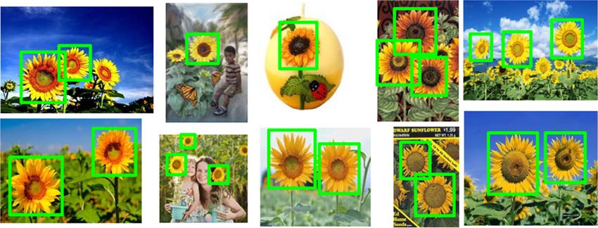
Optical Engineering 52(9), 093105 (September 2013)

                Object detection using voting spaces trained by few
                samples
                Pei Xu                                                              Abstract. A method to detect generic objects by training with a few image
                Mao Ye                                                              samples is proposed. A new feature, namely locally adaptive steering
                University of Electronic Science and Technology                     (LAS), is proposed to represent local principal gradient orientation infor-
                  of China                                                          mation. A voting space is then constructed in terms of cells that represent
                School of Computer Science and Engineering                          query image coordinates and ranges of feature values at corresponding
                611731, China                                                       pixel positions. Cell sizes are trained in voting spaces to estimate the tol-
                E-mail: cvlab.uestc@gmail.com                                       erance of object appearance at each pixel location. After that, two detec-
                                                                                    tion steps are adopted to locate instances of object class in a given target
                Xue Li                                                              image. At the first step, patches of objects are recognized by densely vot-
                University of Queensland                                            ing in voting spaces. Then, the refined hypotheses step is carried out to
                School of Information Technology and Electrical                     accurately locate multiple instances of object class. The new approach is
                  Engineering                                                       training the voting spaces based on a few samples of the object. Our
                4345, Australia                                                     approach is more efficient than traditional template matching approaches.
                                                                                    Compared with the state-of-the-art approaches, our experiments confirm
                                                                                    that the proposed method has a better performance in both efficiency and
                Lishen Pei                                                          effectiveness. © The Authors. Published by SPIE under a Creative Commons Attribution
                Pengwei Jiao                                                        3.0 Unported License. Distribution or reproduction of this work in whole or in part requires full
                University of Electronic Science and Technology                     attribution of the original publication, including its DOI. [DOI: 10.1117/1.OE.52.9.093105]
                   of China
                School of Computer Science and Engineering                          Subject terms: several samples; voting spaces; object detection.
                611731, China                                                       Paper 130809 received Jun. 3, 2013; revised manuscript received Aug. 5, 2013;
                                                                                    accepted for publication Aug. 9, 2013; published online Sep. 16, 2013.

                1 Introduction                                                                      computational efficiency.In Ref. 16, the authors constructed
                Object detection from a target image has attracted increasing                       an inverted location index (ILI) strategy to detect the instance
                research attention because of a wide range of emerging                              of an object class in a target image or video. This ILI struc-
                new applications, such as those on smart mobile phones.                             ture saves the feature locations of one sample and indexes
                Traditionally, pattern recognition methods are used to train                        feature values according to the locations to locate the object
                a classifier with a large number, possibly thousands, of image                      in target image. But this ILI structure just processes one sam-
                samples.1–10 An object in a sample image is a composite of                          ple. In order to improve the efficiency and accuracy based on
                many visual patches or parts recognized by some sparse fea-                         a small number of training samples, these methods have to
                ture analysis methods. In the detection process, sparse fea-                        run a few times on each of those samples.
                tures are to be extracted in a testing image and a trained                              Different from the dense feature like LARK, key-point
                classifier is used to locate objects in a testing image.                            sampled local features, such as scale invariant feature trans-
                Unfortunately, in most real applications there are always                           form (SIFT)17 and speeded up robust features (SURF),18
                insufficient training samples for robust object detection.                          always obtain a good performance in the case of using thou-
                Most likely, we may just have a few samples about the object                        sands of samples to train classifiers. And these key-point fea-
                we are interested in, such as the situations in passport control                    tures are always in a high-dimensional feature space. If one
                at airports, image retrieval from the Web, and object detec-                        has thousands of samples and needs to learn classifiers such
                tion from video or images without preprocessed indexes. In                          as support vector machine (SVM),3,8 key-point features have
                these cases, the template matching approach based on a small                        obtained good performance. Previous works15,19–21 pointed
                number of samples often has been used.                                              out that the densely sampled local features always give better
                    Designing a robust template matching method remains a                           results in classification tasks than that of key-point sampled
                significant effort.11 Most template matching approaches use                         local features like SIFT17 and SURF.18
                query image to locate instances of the object by densely sam-                           Recently, some interesting researches based on few sam-
                pling local features. Shechtman and Irani provided a single-                        ples have emerged. Pishchulin et al. proposed a person detec-
                sample method12 that uses a template image to find instances                        tion model from a few training samples.22 Their work employs
                of the template in a target image (or a video). The similarity                      a rendering-based reshaping method in order to generate thou-
                between the template and a target patch is computed by a                            sands of synthetic training samples from only a few persons
                local self-similarity descriptor. In Refs. 13 and 14, one sam-                      and views. However, the samples are not well organized and
                ple, representing human behavior or action, is used to query                        their method is not applicable on generic object detection. In
                videos. Based on this training-free idea, Seo and Milanfar                          Ref. 23, a new object detection model is proposed named the
                proposed the locally adaptive regression kernels (LARK)                             fan shape model (FSM). FSM uses a few samples very effi-
                feature as the descriptor to match with the object in a target                      ciently, which handles some of the samples to train out the
                image using only one template.15 This LARK feature, which                           tolerance of object shape and makes one sample the template.
                is constructed by local kernels, is robust and stable, but this                     However, FSM method is not scalable in terms of samples and
                LARK feature brings overfitting problem and results in low                          is only for contour matching.

                Optical Engineering                                                       093105-1                                                   September 2013/Vol. 52(9)

Downloaded From: https://www.spiedigitallibrary.org/journals/Optical-Engineering on 28 Dec 2020
Terms of Use: https://www.spiedigitallibrary.org/terms-of-use
Xu et al.: Object detection using voting spaces trained by few samples

                    In this paper, we propose a novel approach for generic                                    This paper is structured as follows. Section 2 gives an
                object detection based on few samples. First, a new type                                   overview of our method. In Sec. 3, we propose LAS feature.
                of feature at each pixel is considered, called locally adaptive                            Section 4 describes the concept of voting space and the train-
                steering (LAS) feature, which is designed for a majority vot-                              ing processing. Section 5 introduces the procedure of object
                ing strategy. The LAS feature at 1 pixel can describe the local                            matching in voting spaces. Section 6 gives the experimental
                gradient information in the neighborhood, which consists of                                results and compares our method with the state-of-the-art
                the dominant orientation energy, the orthogonal dominant                                   methods. This paper is extended from an early conference
                orientation energy, and the dominant orientation angle.                                    paper31 with improved algorithms and comprehensive exper-
                Then, for each member of this feature, a cell is constructed                               imental results.
                at each pixel of the template image, whose length is the range
                of the feature member value. The cells for all pixels construct                            2 Overview of Our Approach
                a voting space. Since this feature is in three dimensions, three                           An overview of our method is shown in Fig. 1. In the training
                voting spaces are to be constructed. We use a few samples to                               processing, for each dimension of LAS feature, a voting
                train these voting spaces, which represent the tolerance of                                space is constructed by image coordinates ðx; yÞ and corre-
                appearance of an object class at each pixel location.                                      sponding value ranges of the feature member. Each cell in the
                    Our idea of using a LAS feature is motivated by earlier                                voting space is formed by the corresponding pixel position
                work on adaptive kernel regression24 and the work of LARK                                  and its value range of this feature member, which is trained
                feature.15 In Ref. 24, to perform denoising, interpolating, and                            by several samples. Since the voting space is three dimen-
                deblurring efficiently, localized nonlinear filters are derived                            sional (3-D), for simplicity we use a 3-D box to represent
                that adapt themselves to the underlying local structure of the                             a cell. The longer the box is, the higher the cell length.
                image. LARK feature can describe the local structure very                                  The different sizes of boxes mean the different tolerances
                well. After densely extracting LARK features from template                                 of object appearance changes at corresponding pixels. In
                and target images, matrix cosine similarity is used to measure                             Fig. 1, LAS feature ðL; S; θÞ is specially designed for object
                the similarity between query image and a patch from target                                 matching in voting spaces, where L, S, and θ represent the
                image. This method is resilient to noises and distortions, but                             dominant orientation energy, the orthogonal dominant orien-
                the computation of LARK features is time-consuming with                                    tation energy, and the dominant orientation angle, respec-
                heavy memory usage. Our LAS feature simplifies the com-                                    tively, in the neighborhood at each location. Thanks to the
                putation of LARK and saves the memory. Moreover, LAS                                       merit of voting, only a few samples (2 to 10 samples in
                feature also exactly captures the local structure of a specific                            this paper) are enough to train cells.
                object class.                                                                                  In the detection process, by randomly choosing one sam-
                    Our voting strategy is inspired by the technology of                                   ple image as the query Q, the instances of an object class are
                Hough transformation. Many works25–30 have contributed                                     located in target image T, which is always larger than Q.
                to model spatial information at locations of local features                                First, the patches T i extracted from T by a sliding window
                or parts as opposite to the object center by Hough voting.                                 are detected by densely voting in the trained voting spaces.
                The Hough paradigm starts with feature extraction and                                      Each component of LAS feature of T i and Q is voted in each
                each feature casts votes for possible object positions.4                                   voting space to obtain a value of similarity. If the values of
                There are two differences from Hough voting. The first                                     similarity of all LAS features are larger than the correspond-
                one is each cell size of the voting spaces is trained out by                               ing thresholds, then T i is a similar patch of Q. Then a refined
                samples. But each cell size of the Hough voting space is                                   hypotheses step is used to accurately locate the multiple
                all fixed. Our trained space can tolerate more deformation.                                instances by computing the histogram distance correspond-
                The second one is our voting strategy is based on template                                 ing to the feature θ. The refined step is just processing the
                matching. Previous Hough voting is based on a trained code-                                similar patches that are obtained in the voting step. If
                book with thousands of samples.                                                            the histogram distance of θ between a similar patch and

                                                                        Training Voting Spaces Part
                                                                                                                Voting Spaces

                                                                                   Voting
                                                                                                       ∆                ∆        ∆Θ
                                                                                                           ∆L           ∆S           ∆θ
                                                                                   Spaces
                                                                                  Training                      y            y            y

                                                                                                       x                         x
                                                                                                                    x

                                                                                                            Detection Part
                                                     Query                        ( LQ , SQ ,θQ )
                                                       Q
                                                               Locally Adaptive                       Voting
                                                                                                                              Refined
                                                               Steering Feature                     On Trained               Hypotheses
                                                                 Computation                          Spaces
                                                     Target                       ( LT , ST ,θT )
                                                       T

                Fig. 1 The overview of our method. In the trained voting spaces, ðx ; y Þ means the query image coordinates. Each bin in the spaces is corre-
                sponding to the pixel cell.

                Optical Engineering                                                            093105-2                                          September 2013/Vol. 52(9)

Downloaded From: https://www.spiedigitallibrary.org/journals/Optical-Engineering on 28 Dec 2020
Terms of Use: https://www.spiedigitallibrary.org/terms-of-use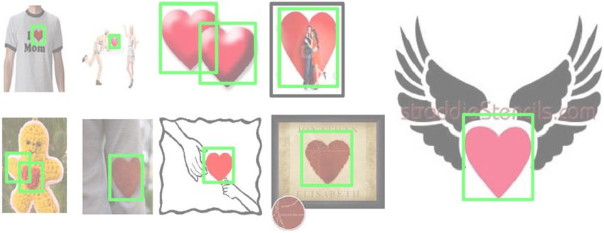
Xu et al.: Object detection using voting spaces trained by few samples


                Q is small enough, then the similar patch is the object                                          λ1   0
                                                                                                  Λði;jÞ ¼                :                                          (2)
                instance.                                                                                        0    λ2

                                                                                                     The eigenvalues λ1 and λ2 represent the gradient energies
                3 Locally Adaptive Steering Feature                                               on the principal and minor directions, respectively. Our LAS
                The basic idea of our LAS is to obtain the locally dominant                       feature at each pixel is denoted as ðLði;jÞ ; Sði;jÞ ; θði;jÞ Þ. We
                gradient orientation of image. For gray image, we compute                         define a measure Lði;jÞ to describe the dominant orientation
                the gradient directly. If the image is RGB, the locally dom-                      energy as follows:
                inant gradient orientation is almost the same on each chan-
                nel. To reduce the computation cost of transforming RGB to                                        λ1 þ ξ 0
                                                                                                  Lði;jÞ ¼ 2 ·             ;   ξ 0 ≥ q0 ;                            (3)
                gray image, we just use the first channel of RGB. The dom-                                        λ2 þ ξ 0
                inant orientation of the local gradient field is the singular
                vector corresponding to the smallest singular value of the                        where ξ 0 is the tunable threshold that can eliminate the effect
                local gradient matrix.24,32 (The proof of transformation                          of noise. The parameter q0 is a tunable threshold. The mea-
                invariance of singular value decomposition (SVD) can be                           sure Sði;jÞ describes the orthogonal direction energy with
                reviewed by interested readers from Ref. 24.) For each                            respect to Lði;jÞ .
                pixel ði; jÞ, one can get the local gradient field shown in
                Fig. 2(a). The local gradient field is a patch in the gradient                                    λ2 þ ξ 0
                map around the pixel ði; jÞ. Here, the size is set as                             Sði;jÞ ¼ 2 ·             :                                         (4)
                                                                                                                  λ1 þ ξ 0
                3 × 3 pixels. The dominant orientation means the principal
                gradient orientation in this gradient field. To estimate the                         The measure θði;jÞ is the rotation angle of Lði;jÞ , which
                dominant orientation, we compute the horizontal and                               represents the dominant orientation angle.
                orthogonal gradients of the image. Then, the matrix
                GFði; jÞ is concatenated column-like as follows:                                  θði;jÞ ¼ arctanðv1 ∕v2 Þ;                                          (5)

                                                                                                  where ½v1 ; v2 T is the second column of V ði;jÞ .
                               2                                               3                     The LAS feature can describe the local gradient distribu-
                                   gx ði − 1; j − 1Þ      gy ði − 1; j − 1Þ                       tion information (see Fig. 2). L, S, and θ are from the com-
                           6                  ..                    ..      7
                           6                   .                     .      7                     putation of the local gradient field, which can yield
                           6                                                7
                GFði; jÞ ¼ 6
                           6             gx ði; jÞ             gy ði; jÞ    7;
                                                                            7           (1)       invariance to brightness change, contrast change, and
                           6                 ..                    ..       7                     white noise as shown in Fig. 3. The results of Fig. 3 are
                           4                  .                     .       5                     from the computation of LAS feature under different corre-
                                   gx ði þ 1; j þ 1Þ      gy ði þ 1; j þ 1Þ                       sponding conditions. Due to the SVD decomposition of local
                                                                                                  gradients, the conditions of Fig. 3 on each pixel do not
                                                                                                  change the dominant orientation energy enormously. One
                                                                                                  can find the proof details of the tolerance of white noises,
                where gx ði; jÞ and gy ði; jÞ are, respectively, gradients of                     brightness change, and contrast change from Ref. 24.
                the x and y directions at the pixel ði; jÞ. The principal direc-                     Some studies15,19–21 have already pointed out that the
                tion is computed by SVD decomposition GFði; jÞ ¼                                  densely sampled local features always give better results
                U ði;jÞ Λði;jÞ V Tði;jÞ , where Λði;jÞ is a diagonal 2 × 2 matrix                 in classification tasks than that of key-point sampled local
                given by                                                                          features, such as SIFT17 and SURF.18 These key-point

                                                                                                                         Original Image
                                                     Si

                                              θi

                                                                                                             L                 S            θ
                                                Li

                                                                         (a)                                                       (b)

                Fig. 2 (a) Locally adaptive steering (LAS) feature at some pixels. The red dots mean the positions of pixels. The ellipse means the dominant
                orientation in the local gradient patch around the corresponding pixel. (b) The components of LAS feature in an image. L, S, and θ are
                shown as a matrix, respectively.

                Optical Engineering                                                       093105-3                                              September 2013/Vol. 52(9)

Downloaded From: https://www.spiedigitallibrary.org/journals/Optical-Engineering on 28 Dec 2020
Terms of Use: https://www.spiedigitallibrary.org/terms-of-use
Xu et al.: Object detection using voting spaces trained by few samples
White Gaussian
Original Brightness Change Contrast Change
Noise
L 1.5446 L 1.5445 L 1.5462 L 1.5436
S 0.6474 S 0.6475 S 0.6467 S 0.6478
Original Brightness Change
θ 49.46 θ 49.41 θ 49.45 θ 49.46
L 1.9358 L 1.9335 L 1.9333 L 1.9349
S 0.5166 S 0.5171 S 0.5172 S 0.5168
White Gaussian
Contrast Change
Noise θ -17.11 θ -17.13 θ -17.10 θ -17.12
L 1.4417 L 1.4412 L 1.4419 L 1.4418
S 0.6936 S 0.6938 S 0.6935 S 0.6936
θ -76.97 θ -76.93 θ -76.94 θ -76.95
Fig. 3 Robustness of the LAS feature in different conditions. The sigma of Gaussian noise is 4.
sampled features are always in a high-dimensional feature LARK,15 there is only gradient energy information, which
space in which no dense clusters exist.15 Comparing to cannot reflect the energy variations. For HOG,27 there are
the histogram of gradient (HOG) feature,27 our LAS feature just values of region gradient intensity in different gradient
has smaller memory usage. Each location of the HOG feature orientations, which cannot reflect dominant orientation
is 32 dimensions histogram, while our LAS feature is just energy and angle.
three dimensions. In Ref. 33, the authors also proposed dom-
inant orientation feature. But this dominant orientation is a 4 Training Voting Spaces
set of representative bins of the HOG.33 Our dominant gra- The template image coordinates and the value ranges of the
dient orientation is computed by the SVD decomposition of LAS feature component at the corresponding locations form
the local gradient values, which have more local shape infor- the voting spaces (denoted as ΔL, ΔS, and ΔΘ, respectively,
mation. Comparing to the LARK feature,15 our LAS feature for three components of LAS feature). To match the template
has 27 times smaller memory usage, for the LARK feature is image and the patch from the target image (testing image)
81 dimensions at each pixel location. In Ref. 24, the authors accurately, the cell length should be trained to reflect the tol-
mentioned these three parameters, but no one has used them erance of appearances at each pixel location. Several samples
as features. Next, we train the voting spaces based on this (2 to 10 samples in this paper) are enough to train the cells in
LAS feature to obtain three voting spaces. each voting space.
So why can the LAS deal with only a few image samples Assume the query samples as Q ¼ fQ1 ; Q2 ; : : : ; Qn g and
well? That is because our LAS feature contains more local n is the cardinality of Q. We use Eqs. (3) to (5) to compute
gradient information than other dense features like LARK15 the LAS feature matrices of nðn ≥ 2Þ samples and obtain
and HOG.27 There are three components of our LAS feature L ¼ fL1 ; L2 ; : : : ; Ln g, S ¼ fS1 ; S2 ; : : : ; Sn g, and Θ ¼
Lði;jÞ , Si;j , and θi;j , which represent the dominant orientation fθ1 ; θ2 ; : : : ; θn g. We want to get the tolerance at each loca-
energy, the orthogonal direction energy of dominant orien- tion from the matrices Li , Si , and θi for (i ¼ 1; 2; : : : ; n).
tation, and the dominant orientation angle, respectively. For Because our LAS feature is from local gradients at each loca-
tion, each value in matrices Li , Si , and θi reflects the local
edge orientation. To reflect the variation range of samples at
LAS Feature
each location, we define the cell sizes ΔL, ΔS, and Δθ as
{
Q Ti |L Q ) = 0.6167
Voting Result
p( i follows:
p( i |S Q ) = 0.6417
|θ Q ) = 0. 5431 ΔLðj;kÞ ¼ max Li − min Li ; (6)
i¼1;2;: : : ;n ðj;kÞ i¼1;2;: : : ;n ðj;kÞ
p( i
{
Q Tj p( |L Q ) = 0.8311
j
Voting Result
p( j |S Q ) = 0.8289 ΔSðj;kÞ ¼ max Si − min Si ; (7)
i¼1;2;: : : ;n ðj;kÞ i¼1;2;: : : ;n ðj;kÞ
p( j |θ Q ) = 0. 8094
{
Q Tk p( k |LQ ) = 0.6231
Voting Result Δθðj;kÞ ¼ max θi − min θi ; (8)
p( k |S Q ) = 0.6408 i¼1;2;: : : ;n ðj;kÞ i¼1;2;: : : ;n ðj;kÞ
p( k |θQ ) = 0. 6011
where ðj; kÞ is the pixel position in the template.
Our definition of cell size is not the only choice. However,
Fig. 4 Voting results comparison between Q and different patches
from T. The thresholds τL ¼ 0.7812, τS ¼ 0.7793, and τθ ¼ 0.7704 this definition is very simple and effective. Different from
are computed by Eqs. (15) to (17). The patch T j is the similar one traditional training scheme, our training method, based on
and the voted result is bounded by the red box. LAS feature, is not computationally expensive.
Optical Engineering 093105-4 September 2013/Vol. 52(9)
Downloaded From: https://www.spiedigitallibrary.org/journals/Optical-Engineering on 28 Dec 2020
Terms of Use: https://www.spiedigitallibrary.org/terms-of-use
Xu et al.: Object detection using voting spaces trained by few samples
5 Object Detection H1 ∶T 1 is similar to Q,
A query image Q is randomly selected from the sample H2 ∶T 2 is similar to Q,
images. And the target image T is divided into a set of over- HN T ∶T N T is similar to Q.
lapping patches T ¼ fT 1 ; T 2 ; · · · ; T N T g by a sliding win-
dow with the same size as the query image Q, where N T Because there are three components with respect to the
is the number of patches in T . LAS feature, we have three estimated conditional densities
In our object matching scheme, there are two steps to pðHi jLQ Þ, pðHi jSQ Þ, and pðHi jθQ Þ. These conditional den-
search similar patches in T . First step is voting in the trained sities are defined as the results of voting. Specifically,
voting spaces (see Fig. 5). To combine the votes from three
voting spaces, we use a joint voting strategy to detect similar KðLQ ; LT i Þ
patches from T . After the first step, one can get some similar pðHi jLQ Þ ¼ ; (9)
kQk
patches T 0 ¼ fT 10 ; T 20 ; · · · ; T 0 T 0 g (T 0 ⊂ T and N T0 is the
N
cardinality of T 0 ). Then a refined hypotheses step follows.
In this step, the histogram distance of the LAS feature
0
between Q and T i0 ði ¼ 1; 2; · · · ; N T Þ is used to measure KðSQ ; ST i Þ
pðHi jSQ Þ ¼ ; (10)
integral similarity, which can precisely locate the instances kQk
of the query Q.
5.1 Voting in Trained Spaces KðθQ ; θT i Þ
pðHi jθQ Þ ¼ ; (11)
We associate each patch in T with a hypothesis as kQk
follows:
where kQk is the number of pixels of the image Q, and
Query Target Kð:; :Þ is a map: R2 × R2 → Zþ , which counts the votes in
(a) the corresponding space.
To compute the function Kð:; :Þ, we define three variables
Training Spaces
Samples ΔL ð∈ ΔLÞ, ΔS ð∈ ΔSÞ, and Δθ ð∈ ΔΘÞ as ΔL ¼ jLQ − LT i j,
ΔS ¼ jSQ − ST i j, and Δθ ¼ jθQ − θT i j, where j:j means to
take absolute value of the elements in the matrix. In our
framework, the functions KðLQ ; LT i Þ, KðSQ ; ST i Þ, and
KðθQ ; θT i Þ are defined as
X
(b) Combination Voting: KðLQ ; LT i Þ ¼ sgnðΔLðj;kÞ − ΔLðj;kÞ Þ; (12)
p( i | LQ ) ≥ τ L , p( i | SQ ) ≥ τ S , p( i | θQ ) ≥ τ θ j;k
If a p atch is similar to Q , then:
(Q , i ) = 1. X
KðSQ ; ST i Þ ¼ sgnðΔSðj;kÞ − ΔSðj;kÞ Þ; (13)
j;k
X
KðθQ ; θT i Þ ¼ sgnðΔθðj;kÞ − Δθðj;kÞ Þ; (14)
j;k
where ΔLðj;kÞ , ΔSðj;kÞ , and Δθðj;kÞ are the trained cell matri-
ces in the previous section. For the component L of LAS
(c) Histogram Distance:
feature, if ΔLðj;kÞ ≥ ΔLðj;kÞ , then sgnðΔLðj;kÞ − ΔLðj;kÞ Þ ¼
1 at the pixel location ðj; kÞ. This means a vote added to
(h )
2
T′
T j′
M
Q
m − hmj the result of KðLQ ; LT i Þ. From Eqs. (12) to (14) of function
χ (h , h ) =
2 Q
T′
≤ τ h , j = 1, 2, , N T′ Kð:; :Þ, we can find that the estimated conditional densities in
m =1 hmQ + hmj
Eqs. (9) to (11) represent, for each LAS component, the ratio
of votes at the size of the query image Q.
The estimated conditional densities pðHi jLQ Þ, pðHi jSQ Þ,
and pðHi jθQ Þ between Q and each element of T are com-
puted after voting. So how can we discriminate the similar
patches from these densities?
Our answer is organizing the samples to train the density
thresholds between Q and the set Q. In Ref. 15, the authors
use a tunable threshold to detect possible objects presented in
the target image and nonmaxima suppression strategy to
locate the objects in a similarity potential map. But in our
Fig. 5 (a) The query, target, and training samples. (b) Voting results in scenario, we make use of several samples sufficient to obtain
the target image. (c) Refined hypotheses step. the thresholds, written as τL , τS , and τθ , off-line. These three
Optical Engineering 093105-5 September 2013/Vol. 52(9)
Downloaded From: https://www.spiedigitallibrary.org/journals/Optical-Engineering on 28 Dec 2020
Terms of Use: https://www.spiedigitallibrary.org/terms-of-use
Xu et al.: Object detection using voting spaces trained by few samples
thresholds must contain two properties. The first one is that to describe the integral information of the object. The con-
these thresholds reflect the tolerance of the cells. The second struction of LAS feature shows that θ is related to the ori-
one is that the thresholds must be different when the query entation of the local edge, which is mentioned in Ref. 24.
image changes. Here, the computation formulas of τL , τS , To use the contour information sufficiently, we compute
and τθ are the following: the histogram distance between θQ and θT i0 . For the features
θQ and θT i0 , after being quantized here in the bin of 10 deg,
KðLQ ; LQi Þ one can calculate the histograms denoted as hQ and hT i ,
0
τL ¼ min ; (15) T i0
i¼1;: : : ;n kQk Q
respectively. The distance between h and h is defined as
Ti 2 0
KðSQ ; SQi Þ X
M
ðhQ
m − hm Þ
τS ¼ min (16) 2 T i0
; χ ðh ; h Þ ¼
Q
; (21)
i¼1;: : : ;n kQk m¼1 m þ hm
hQ i T0
KðθQ ; θQi Þ where M is the number of bins of the histogram. We also use
τθ ¼ min ; (17)
i¼1;: : : ;n kQk a few samples to train the threshold of histogram distance,
which can be written as τh . More specifically,
where Qi ∈ Q. In previous section, we showed that the vot-
ing spaces are trained by the sample set Q, so the tolerance of X
M
ðhQ
Qj 2
m − hm Þ
the cells is reflected in τL , τS , and τθ . When the query image τh ¼ max Q
: (22)
m þ hm
hQ
j¼1;: : : ;n j
changes, we can see from Eqs. (15) to (17) that τL , τS , and τθ m¼1
are also changed. It is worth noting that the min function is
just one of the alternative functions in Eqs. (15) to (17). The more similar two histograms are, the smaller χ 2 is. So
0
One can choose mean function, median function, even we use the max function to compute the τh . If χ 2 ðhQ ; hT i Þ ≤
0
max function, or so on. The reason that we choose min func- τh is satisfied, T i will be the instance of the query Q. It is
tion is that our samples in the experiment are without rota- efficient to use the χ 2 distance [see Fig. 5(c)]. The reason is
tion, strong noises, and brightness change. Other functions to that the histogram distance between Q and T i0 reflects the
handle more complex cases need further research. In our integral difference.
experiments, we just use Eqs. (15) to (17) to compute the In fact, besides using the histogram distance of θ, we can
thresholds. also use the histogram distance of L and S. But in experi-
Next, we use the estimated conditional densities and ments, we find that using the histogram distance of L or
trained thresholds to obtain the similar patches. For the S cannot enhance the precision of detection result, and θ
LAS feature containing three components, our work is to is better than L and S. The reason is that the feature θ
combine these three components to detect the similar patches more precisely describes the contour information of an
T j0 . So we define a map Fk ðQ; Hi Þ∶ð0; 1Þ Q→ f0; 1g (k ¼ 1, object.
2, 3) and the combination F ðQ; Hi Þ ¼ 3k¼1 Fk , where Previous works3,34–38 have already shown that the histo-
gram is a popular representation for feature description. That
1 pðHi jLQ Þ ≥ τL ; is because the histogram encodes the distribution of spatially
F1 ðQ; Hi Þ ¼ (18)
0 otherwise; unordered image measurements in a region.36 The χ 2 dis-
tance is used to compare the distance between two histo-
grams in Ref. 3. So, we use this quadratic-χ measurement
to discriminant histogram distance.
1 pðHi jSQ Þ ≥ τS ;
F2 ðQ; Hi Þ ¼ (19)
0 otherwise;
6 Experimental Results
The experiments consist of three parts using car detection,
1 pðHi jθQ Þ ≥ τθ . face detection, and generic object detection, respectively.
F3 ðQ; Hi Þ ¼ (20)
0 otherwise: To handle object variations on scale and rotation in the target
image, we use the strategies provided in Ref. 15, which con-
For each T i ∈ T , if Fk ðQ; Hi Þ ¼ 1, ∀ k ¼ 1, 2, 3, then struct a multiscale pyramid of the target image and generate
FðQ; Hi Þ ¼ 1. In Fig. 4, we show the voting results between rotated templates (from Q) in 30-deg steps. The receiver
Q and the elements in T . The densities in the red bounding operating characteristic (ROC) curves are drawn to describe
box are all larger than the thresholds. So T j is the patch sim- the performance of object detection methods. We use the def-
ilar to Q. We compute the combination function F for all inition in Ref. 15 that Recall and Precision are computed as
T i ði ¼ 1; 2; · · · ; N T Þ and put patches whose function values
equal to 1 into the set T 0 . In Fig. 5, we draw the graphical TP TP
illustration of the detection process. Recall ¼ ; Precision ¼ ; (23)
nP TP þ FP
5.2 Refined Hypotheses Step where TP is the number of true positive, FP is the number of
After the density voting step, we obtain the similar patch set false positive, and nP is the total number of positive in the
T 0 . The refined step just a process of this set T 0 , which is test data set. And 1 − Precision ¼ FP∕ðTP þ FPÞ. In the fol-
obtained from the voting. However, the first step is just a lowing experimental results on each data set, we will present
local voting method at each pixel location. It is not enough Recall versus 1 − Precision curves.
Optical Engineering 093105-6 September 2013/Vol. 52(9)
Downloaded From: https://www.spiedigitallibrary.org/journals/Optical-Engineering on 28 Dec 2020
Terms of Use: https://www.spiedigitallibrary.org/terms-of-use
Xu et al.: Object detection using voting spaces trained by few samples

                                                  Query

                                              Training Cell
                                                Samples

                                                         Fig. 6 The detection results of UIUC car on the single-scale test set.

                6.1 Car Detection                                                                 querying the object using the training samples one by
                Now, we show the performance of our method on the                                 one. But this is not our main point. Our focus is that detecting
                University of Illinois at Urbana-Champaign (UIUC) car                             the instances of an object by one query using our method is
                data set.39 The UIUC car data set contains the learning                           competitive to or better than that of the one-query method
                and test sets. The learning set consists of 550 positive car                      executing several times. Compared with the LARK method,
                images and 500 noncar images. The test set consists of                            because we organize the training samples reasonably, our
                two parts: 170 gray-scale images containing 200 side                              detection results have more appearance tolerance of the
                views of cars of size 100 × 40 and 108 gray-scale images                          object. Although we just have few samples in hand, the
                containing 139 cars.                                                              detection result of our method is better than that of the pre-
                    In Fig. 6, we show some detected examples of UIUC car                         vious works,39 which need hundreds or thousands of
                on the single-scale test set with the trained parameters                          samples.
                τL ¼ 0.7042, τS ¼ 0.7031, τθ ¼ 0.6852, and τh ¼ 251.5.                               The comparisons of detected equal-error rates (EER)15 are
                The query image and training samples are of size 100 × 40.                        shown in Tables 1 and 2. One can also find that our proposed
                    To demonstrate the performance improvement of our                             method is competitive to or better than those state-of-the-art
                method, we compare our method to some state-of-the-art                            methods. Here, we compare our method to the state-of-the-
                works15,39–41 (see Fig. 7). Seo et al.15 proposed the LARK                        art training-based methods3,39–41 and the one-query method
                features that detect instances of the same object class and
                get the best accuracy detection, resulting in template match-                                1
                ing methods. This method is referred to as LARK. In Ref. 39,
                the authors used a sparse, part-based representation and gave
                an automatically learning method to detect instances of the                                0. 8
                object class. Wu et al.41 showed a method based on the per-
                pixel figure-ground assignment around a neighborhood of
                                                                                                                                                    Agarwal et al.
                the edgelet on the feature response. Their method needs                                    0. 6
                                                                                                  Recall

                to learn the ensemble classifier with a cascade decision strat-
                                                                                                                                                    H.J.Seo et al.
                egy from the base classifier pool.41 In Ref. 40, the authors
                introduced a conditional model for simultaneous part-                                      0. 4
                                                                                                                                                    Kapoor and
                based detection and segmentation of objects of a given                                                                                Winn
                class, which needs a training set of images with segmentation                                                                       Our method
                                                                                                           0. 2
                masks for the object of interest. However, these works39,40,41
                are all based on the training methods, which need hundreds                                                                         Wu and Nevatia
                or thousands of samples.
                                                                                                             0
                    From Fig. 7, it can be observed that our method is better                                     0   0. 2           0. 4          0. 6              0. 8
                than the methods in Refs. 15 and 39 and the recall is lower                                                       1-Precision
                than that in Refs. 40 and 41, which need hundreds or thou-                        Fig. 7 Comparison of receiver operating characteristic (ROC) curves
                sands of samples. The precision of our method can be                              between our method and the methods in Refs. 15, 39, 40, and 41 on
                improved more if the detected results are combined by                             the UIUC single-scale test set.

                Optical Engineering                                                       093105-7                                          September 2013/Vol. 52(9)

Downloaded From: https://www.spiedigitallibrary.org/journals/Optical-Engineering on 28 Dec 2020
Terms of Use: https://www.spiedigitallibrary.org/terms-of-use
Xu et al.: Object detection using voting spaces trained by few samples
Table 1 Detection equal-error rates on the single-scale UIUC car test competitive to the methods in Refs. 3, 40, and 41. These
set. methods always need thousands of samples to train classi-
fiers. But our method, whose training processing is much
simpler than that of these methods, just needs several sam-
Ref. 39 77.08%
ples. Compared to these three methods, our method is also
competitive.
Ref. 15 88.12%
Ref. 40 94.0%
6.2 Face Detection
Ref. 3 98.5% In this section, we demonstrate the performance of our
method to face detection on Massachusetts Institute of
Ref. 41 97.5% Technology—Carnegie Mellon University (MIT-CMU)
Our method 92.15% face data set42 and Caltech face data set.11,16 The several
training samples in our face detection experiments are all
chosen from Fundação Educacional Inaciana (FEI) face
data set.43 Since we just have few samples in hand, in this
(LARK). The EER on the single- and multiscale test sets are section the comparison is only made to the template match-
shown in Tables 1 and 2, respectively. From Table 1, it can be ing method. As mentioned before, in the template matching
found that the EER of our method is higher than that of meth- methods, the LARK method15 shows good performance. So
ods in Refs. 15 and 39, and lower than that of the methods in we take it as our baseline object detector.
Refs. 3, 40, and 41. In Table 2, the EER of our method is First, we show the detection results of our strategy on
higher than that of the methods in Refs. 15 and 39 and MIT-CMU face data set. There are 45 images with 157 fron-
lower than that of the methods in Refs. 3 and 40. As our tal faces of various sizes in our test set. The query image and
strategy is based on few samples, the prior knowledge of training samples are all adjusted to the size 60 × 60. The
the object class is limited. However, the EER of our method scale of faces in the data set between the largest and smallest
also reaches 92.15 and 91.34%, respectively, which are is from 0.4 to 2.0. One can see some of the results in Fig. 8.
Although the target image is blurry or contains a cartoon
Table 2 Detection equal-error rates on the multiscale UIUC car test human face, our detection method can localize the faces.
set. Especially in Fig. 9, we detect 56 faces correctly among
57 faces and the precision rate is higher than the results
in Refs. 15 and 44.
Ref. 39 44.08% To make a fair comparison, we use the union LARK
detection results from several images. For example, if
Ref. 15 77.66% there are six training samples, LARK processes them one
by one as the query image. For each target image, we record
Ref. 40 93.5%
the true positives of six queries and get the total number of
true positives without repeat. In this way, this union multi-
Ref. 3 98.6%
samples detection result of LARK can be compared with our
Our method 91.34% method fairly. In Fig. 10, we show the comparison between
our method and LARK.15 The curve of our method is the
Query
Training Cell
Samples
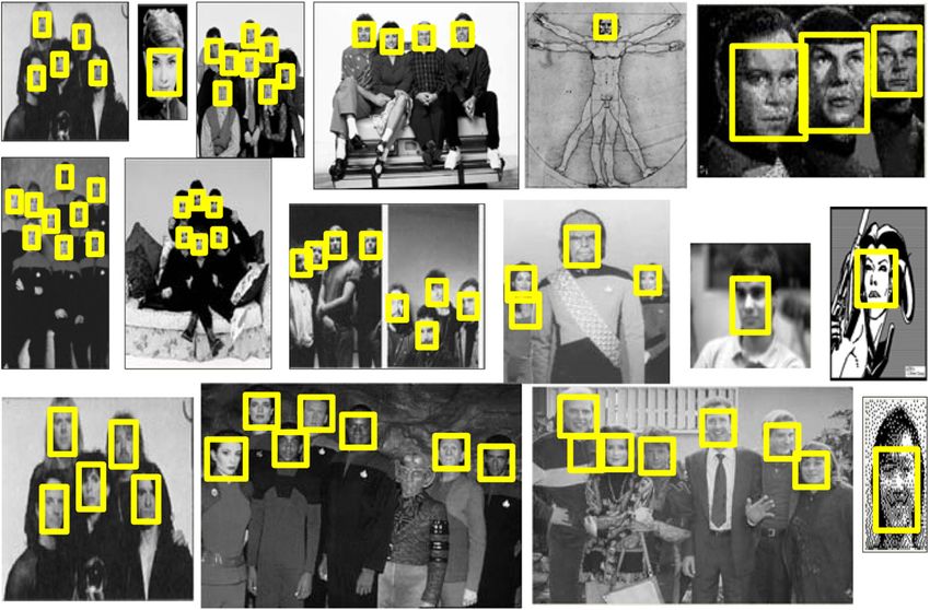
Fig. 8 Detection results on MIT-CMU face data set. Even though the image is blurry, our method also localizes the object. τL ¼ 0.7745,
τS ¼ 0.7688, τθ ¼ 0.7911, and τh ¼ 488.6.
Optical Engineering 093105-8 September 2013/Vol. 52(9)
Downloaded From: https://www.spiedigitallibrary.org/journals/Optical-Engineering on 28 Dec 2020
Terms of Use: https://www.spiedigitallibrary.org/terms-of-use
Xu et al.: Object detection using voting spaces trained by few samples
1
Query
0.96
Recall
0.92
0.88
Training Cell
Samples
0 0.1 0.2 0.3 0.4 0.5 0.6 0.7
1-Precision
Training Cell (a)
Samples
Query 1
Fig. 9 There are 57 faces in the target image, and our method detects
56 faces with five false alarm. τL ¼ 0.7812, τS ¼ 0.7793, τθ ¼ 0.7704,
and τh ¼ 475.1. (1) (2)
0.96
average of five query images with the same training samples.
Recall
One can find that our method is superior to the LARK. (1)
Next, we perform our method on the Caltech11,16 face data (3) (4) (2)
0.92
set, which contains 435 frontal faces in file “Faces” with
(3)
almost the same scale.
The proposed method on three data sets achieves higher (4)
accuracy and a lower false alarm rate than that of the 0.88
0 0.1 0.2 0.3 0.4 0.5 0.6 0.7
union LARK. The organization of the several training samples 1-Precision
is more efficient than the one-by-one detection strategy. We (b)
draw ROC curves with respect to different query images
from the same training samples and to the same query Fig. 11 ROC curves on MIT-CMU face data set. In (a), we show ROC
image on different training samples [see Figs. 11(a) and curves of different query images from the same training samples. In
(b), the ROC curves are drawn with the same query image on different
11(b)] on MIT-CMU face data set. Figure 11 demonstrates training samples.
that our detection strategy can achieve consistent precisions
for both different training samples and different query images.
This means our method is robust on different training samples samples. This is because our detection method has two steps,
and query images. In fact, we also obtained the same result on voting step (VS) and refined hypotheses step (RHS), which
other data sets used in this paper. To describe the result clearly, measure the object locally and integrally, respectively. Here,
we give the ROC curve on the MIT-CMU face data set. we show how these two steps affect our detection results. We
From above, it can be seen that our detection strategy is compare the detection results of VS + RHS, VS and RHS on
consistent and robust on different query images and training the Caltech data set (see Fig. 12). Each curve is drawn and
averaged with the same seven query images and three train-
ing samples. One can see that the combination of both steps
1
can get a higher precision rate than that of using each step
alone, and that the voting strategy along has a higher accu-
0.98 racy than RHS. A similar conclusion can be drawn with other
data sets, which are not shown here.
0.96
6.3 Generic Object Detection
Recall
0.94 We have already shown the detection results of our proposed
Our method method on the car and face data set. In this section, we use
0.92 our strategy to some general real-world images containing
hearts, flowers, and footballs. To the best of our knowledge,
there does not exist a data set for object detection based on a
0.9 Union LARK few samples. So we download some real-world images from
Google as our data set. One can find these images from our
0.88
website http://cvlab.uestc.edu.cn/xupei. There are 34 images
0 0.2 0.4 0.6 0.8 1 of red hearts with 49 positive samples and 40 images of sun-
1-Precision flowers with 101 positive samples. In all of these data sets,
the scale is from 0.2 to 1.8.
Fig. 10 Comparison between our proposed method and the union
locally adaptive regression kernels (LARK) on MIT-CMU data set. The detection examples can be found in Fig. 13. In the
The ROC curve of our proposed method is the average on six real world, the red-heart shape can be found with complex
query images. display. So, our detection results contain some false alarms.
Optical Engineering 093105-9 September 2013/Vol. 52(9)
Downloaded From: https://www.spiedigitallibrary.org/journals/Optical-Engineering on 28 Dec 2020
Terms of Use: https://www.spiedigitallibrary.org/terms-of-useXu et al.: Object detection using voting spaces trained by few samples
1 tcLAS
ρcLAS ¼ ; (24)
tcLAS þ tcLARK
0.9
VS+RHS tcLARK
ρcLARK ¼ ; (25)
tcLAS þ tcLARK
0.8 VS
Recall
RHS
with a similar definition for ρdLAS and ρdLARK as
0.7 tdLAS
ρdLAS ¼ ; (26)
tdLAS þ tdLARK
0.6
tdLARK
ρdLARK ¼ : (27)
tdLAS þ tdLARK
0.5
0 0.2 0.4 0.6 0.8 1
1-Precision One can find the comparison results of LAS and LARK
features in Table 3. In the experiment, we evaluate 10 testing
Fig. 12 Comparison of different steps on the Caltech data set. The times (each testing contains 30 images) to record the evalu-
green curve represents the results that combine both steps. The ation time of the two steps in both our method and the
red curve just uses the voting step. The black curve is using only
refined hypotheses step. LARK, respectively. In Table 3, we can see that the construc-
tion time for LARK feature is more ∼30% than that of our
LAS feature. This is because the LAS feature just needs to
6.4 Time Efficiency Comparison and Feature compute the gradients and SVD decomposition to get three
Comparison parameters. But for LARK feature, after SVD decomposi-
Now we compare the efficiency between our proposed tion, the local kernel must be computed and then the princi-
scheme and the detection scheme.15 For these two methods, pal component analysis (PCA) method is used to reduce the
there are the same two steps: feature construction and object dimension. The superiority of our LAS feature is not just
detection. We compare the time efficiency of these two steps saving memory, but also cutting down the computing
between our strategy and LARK. To formalize the efficiency, steps for each pixel. In Table 3, one can find that ρdLAS is
tcLAS and tcLARK are, respectively, defined as the evaluation also lower ∼20%% than ρdLARK (blue). Our detection step
time of the feature construction. tdLAS and tdLARK are the evalu- is based on the idea of voting. In Ref. 15, the matrix cosine
ation times of the detection step. Here, we define ρcLAP and similarity for each T i and Q is computed. Then, the salience
ρcLARK to describe the time efficiency of LAS and LARK fea- map is constructed which is very time-consuming. In our
tures, respectively, where method, the time of the training step can be ignored. In
Query
Training Cell
Samples
Query
Training Cell
Samples
Fig. 13 Detection results on general object detection.
Optical Engineering 093105-10 September 2013/Vol. 52(9)
Downloaded From: https://www.spiedigitallibrary.org/journals/Optical-Engineering on 28 Dec 2020
Terms of Use: https://www.spiedigitallibrary.org/terms-of-useXu et al.: Object detection using voting spaces trained by few samples
Table 3 Comparison of efficiency between LAS and LARK.
Testing times 1 2 3 4 5 6 7 8 9 10
ρcLARK 71% 72% 71.5% 73% 74% 73% 72% 71% 71% 70%
ρcLAS 29% 28% 28.5% 27% 26% 27% 28% 29% 29% 30%
ρdLARK 58% 59% 57% 60% 61% 59% 61% 62% 59% 60%
ρdLAS 42% 41% 43% 40% 39% 41% 39% 38% 41% 40%
1 method. Our LAS feature has more efficiency and memory
saving than that of LARK. Besides, the strategy we proposed
in this paper gives a method of object detection when the
0.9 samples are limited. Previous template matching method
is to detect objects using samples one by one, while our
method is to organize several samples to detect objects
0.8 CIE
once. In the future, we will extend our work to the problem
Recall
GLOH of multiple-object detection and improve the efficiency
LARK further.
0.7
LAS
Acknowledgments
Shape Context
0.6
SIFT
This work was supported in part by the National Natural
Science Foundation of China (61375038) 973 National
Basic Research Program of China (2010CB732501) and
0.5
0.1 0.2 0.3 0.4 0.5 0.6 0.7 0.8 Fundamental Research Funds for the Central University
1-Precision (ZYGX2012YB028, ZYGX2011X015).
Fig. 14 Comparison of different kinds of features on Shechtman and
Irani’s test set.12 Gradient location-orientation-histogram,45 LARK,15 References
Shape Context,46 SIFT17 and CIE.12 1. S. An et al., “Efficient algorithms for subwindow search in object detec-
tion and localization,” in 2009 IEEE Conf. on Computer Vision and
Pattern Recognition, pp. 264–271 (2009).
the experiments, we find that the consuming time of the 2. G. Csurka et al., “Visual categorization with bags of keypoints,” in Proc.
European Conf. on Computer Vision, pp. 1–22, Springer, New York
training step isXu et al.: Object detection using voting spaces trained by few samples
15. H. J. Seo and P. Milanfar, “Training-free, generic object detection using 45. K. Mikolajczyk and C. Schmid, “A performance evaluation of local
locally adaptive regression kernels,” IEEE Trans. Pattern Anal. Mach. descriptors,” IEEE Trans. Pattern Anal. Mach. Intell. 27(10), 1615–
Intell. 32(9), 1688–1704 (2010). 1630 (2005).
16. A. Sibiryakov, “Fast and high-performance template matching method,” 46. S. Belongie, J. Malik, and J. Puzicha, “Shape matching and object rec-
in IEEE Conf. on Computer Vision and Pattern Recognition, pp. 1417– ognition using shape contexts,” IEEE Trans. Pattern Anal. Mach. Intell.
1424 (2011). 24(4), 509–522 (2002).
17. D. Lowe, “Distinctive image features from scale-invariant keypoints,”
Int. J. Comput. Vis. 60(2), 91–110 (2004).
18. H. Bay, T. Tuytelaars, and L. Gool, “SURF: speeded up robust features,” Pei Xu received his BS degree in computer
in Proc. European Conf. Computer Vision, pp. 404–417, Springer, New science and technology from SiChuan Uni-
York (2006). versity of Science and Engineering, ZiGong,
19. O. Boiman, E. Shechtman, and M. Irani, “In defense of nearest-neighbor China, in 2008 and his MS degree in con-
based image classification,” in Proc. IEEE Conf. Computer Vision and densed matter physics from University of
Pattern Recognition, pp. 1–8 (2008).
20. F. Jurie and B. Triggs, “Creating efficient codebooks for visual recog- Electronic Science and Technology of
nition,” in IEEE Int. Conf. on Computer Vision, pp. 604–610 (2005). China, Chengdu, China, in 2011. He is cur-
21. T. Tuytelaar and C. Schmid, “Vector quantizing feature space with a rently a PhD student in University of Elec-
regular lattice,” in Proc. IEEE Int. Conf. on Computer Vision, pp. 1– tronic Science and Technology of China,
8 (2007). Chengdu, China. His current research inter-
22. L. Pishchulin et al., “Learning people detection models from few train- ests include machine learning and computer
ing samples,” in IEEE Conf. on Computer Vision and Pattern vision.
Recognition, pp. 1473–1480 (2011).
23. X. Wang et al., “Fan shape model for object detection,” in IEEE Conf.
on Computer Vision and Pattern Recognition, pp. 1–8 (2012). Mao Ye received his PhD degree in math-
24. H. Takeda, S. Farsiu, and P. Milanfar, “Kernel regression for image ematics from Chinese University of Hong
processing and reconstruction,” IEEE Trans. Image Process. 16(2)
(2007). Kong in 2002. He is currently a professor
25. D. H. Ballard, “Generalizing the Hough transform to detect arbitrary and director of CVLab at University of Elec-
shapes,” Pattern Recogn. 13(2), 111–122 (1981). tronic Science and Technology of China.
26. D. Chaitanya, R. Deva, and F. Charless, “Discriminative models for His current research interests include
multi-class object layout,” Int. J. Comput. Vis. 95(1), 1–12 (2011). machine learning and computer vision. In
27. P. Felzenszwalb, D. McAllester, and D. Ramanan, “A discriminatively these areas, he has published over 70
trained, multiscale, deformable part model,” in IEEE Conf. on Computer papers in leading international journals or
Vision and Pattern Recognition, pp. 1–8 (2008). conference proceedings.
28. B. Leibe, A. Leonardis, and B. Schiele, “Robust object detection by
interleaving categorization and segmentation,” Int. J. Comput. Vis.
77(1–3), 259–289 (2008).
29. K. Mikolajczyk, B. Leibe, and B. Schiele, “Multiple object class detec-
tion with a generative model,” in IEEE Computer Society Conf. on Xue Li is an Associate Professor in the
Computer Vision and Pattern Recognition, pp. 26–36 (2006). School of Information Technology and Elec-
30. J. Gall et al., “Hough forests for object detection, tracking, and action trical Engineering at University of Queens-
recognition,” IEEE Trans. Pattern Anal. Mach. Intell. 33(11), 2188– land in Brisbane, Queensland, Australia.
2202 (2011). He obtained the Ph.D degree in Information
31. P. Xu et al., “Object detection based on several samples with training Systems from the Queensland University of
Hough spaces,” in CCPR 2012, Springer, New York (2012). Technology 1997. His current research inter-
32. X. Feng and P. Milanfar, “Multiscale principal components analysis for ests include Data Mining, Multimedia Data
image local orientation estimation,” in 36th Asilomar Conf. on Signals,
Systems and Computers, pp. 478–482, IEEE, New York (2002). Security, Database Systems, and Intelligent
33. C. Hou, H. Ai, and S. Lao, “Multiview pedestrian detection based on Web Information Systems.
vector boosting,” Lec. Notes Comput. Sci. 4843, 210–219 (2007).
34. S.-H. Cha, “Taxonomy of nominal type histogram distance measures,”
in Proc. American Conf. on Applied Mathematics, pp. 325–330, ACM
Digital Library, New York (2008). Lishen Pei received her BS degree in com-
35. M. Godec, P. M. Roth, and H. Bischof, “Hough-based tracking of non- puter science and technology from Anyang
rigid objects,” in IEEE Int. Conf. on Computer Vision, pp. 81–88 Teachers College, Anyang, China, in 2010.
(2011). She is currently an MS student in the Univer-
36. O. Pele and M. Werman, “The quadratic-chi histogram distance family,” sity of Electronic Science and Technology of
in Proc. of 11th European Conf. on Computer Vision, pp. 749–762, China, Chengdu, China. Her current research
Springer, New York, (2010).
37. B. Schiele and J. L. Crowley, “Object recognition using multidimen- interests include action detection and action
sional receptive field histograms,” in Proc. of European Conf. on recognition in computer vision.
Computer Vision, pp. 610–619, Springer, New York (1996).
38. M. Sizintsev, K. G. Derpanis, and A. Hogue, “Histogram-based search:
a comparative study,” in IEEE Conf. on Computer Vision and Pattern
Recognition, pp. 1–8 (2008).
39. S. Agarwal, A. Awan, and D. Roth, “Learning to detect objects in
images via a sparse, part-based representation,” IEEE Trans Pattern Pengwei Jiao received his BS degree in
Anal. Mach. Intell. 26(11), 1475–1490 (2004). mathematics from Southwest Jiaotong Uni-
40. A. Kappor and J. Winn, “Located hidden random fields: learning dis- versity, Chengdu, China, in 2011. He is cur-
criminative parts for object detection,” Lec. Notes Comput. Sci. 3953, rently a postgraduate student in the
302–315 (2006).
41. B. Wu and R. Nevatia, “Simultaneous object detection and segmenta- University of Electronic Science and Tech-
tion by boosting local shape feature based classifier,” IEEE Trans. nology of China, Chengdu, China. His current
Pattern Anal. Mach. Intell. 26(11), 1475–1498 (2004). research interests are machine vision, visual
42. H. Rowley, S. Baluja, and T. Kanade, “Neural network-based face surveillance, and object detection.
detection,” IEEE Trans. Pattern Anal. Mach. Intell. 20(1), 23–38
(1998).
43. C. E. Thomaz and G. A. Giraldi, “A new ranking method for principal
components analysis and its application to face image analysis,” Image
Vis. Comput. 28(6), 902–913 (2010).
44. G. Gualdi, A. Prati, and R. Cucchiara, “Multistage particle windows for
fast and accurate object detection,” IEEE Trans. Pattern Anal. Mach.
Intell. 34(8), 1589–1640 (2012).
Optical Engineering 093105-12 September 2013/Vol. 52(9)
Downloaded From: https://www.spiedigitallibrary.org/journals/Optical-Engineering on 28 Dec 2020
Terms of Use: https://www.spiedigitallibrary.org/terms-of-useYou can also read