A FOD Detection Approach on Millimeter-Wave Radar Sensors Based on Optimal VMD and SVDD - MDPI
←
→
Page content transcription
If your browser does not render page correctly, please read the page content below
sensors
Article
A FOD Detection Approach on Millimeter-Wave Radar Sensors
Based on Optimal VMD and SVDD
Jun Zhong, Xin Gou, Qin Shu *, Xing Liu                      and Qi Zeng

                                          School of Electrical Engineering, Sichuan University, Chengdu 610000, China; zhongjun55@163.com (J.Z.);
                                          GX199666@163.com (X.G.); liuxing4@126.com (X.L.); zengqi1982@163.com (Q.Z.)
                                          * Correspondence: shuqin@scu.edu.cn; Tel.: +86-186-0800-6161

                                          Abstract: Foreign object debris (FOD) on airport runways can cause serious accidents and huge
                                          economic losses. FOD detection systems based on millimeter-wave (MMW) radar sensors have the
                                          advantages of higher range resolution and lower power consumption. However, it is difficult for
                                          traditional FOD detection methods to detect and distinguish weak signals of targets from strong
                                          ground clutter. To solve this problem, this paper proposes a new FOD detection approach based
                                          on optimized variational mode decomposition (VMD) and support vector data description (SVDD).
                                          This approach utilizes SVDD as a classifier to distinguish FOD signals from clutter signals. More
                                          importantly, the VMD optimized by whale optimization algorithm (WOA) is used to improve the
                                          accuracy and stability of the classifier. The results from both the simulation and field case show the
                                          excellent FOD detection performance of the proposed VMD-SVDD method.

                                          Keywords: FOD detection; MMW radar sensor system; SVDD classifier; the optimal VMD

                                1. Introduction

                                                The foreign object debris (FOD) [1] on airport runways, such as screws, animals,
Citation: Zhong, J.; Gou, X.; Shu, Q.;    stones, plastics and so on, can lead to tragedies of aircraft damage and human mortality.
Liu, X.; Zeng, Q. A FOD Detection
                                          FODs cause severe direct damage and enormous maintenance cost to airport authorities
Approach on Millimeter-Wave Radar
                                          every year around the world. In order to ameliorate this problem, it is urgent to develop a
Sensors Based on Optimal VMD and
                                          reliable, high-efficiency and automatic FOD monitoring system. At present, the UK Tarsier
SVDD. Sensors 2021, 21, 997. https://
                                          system [2], the Israeli FODetect system [3], the US FODFinder system [4], and the FOD
doi.org/10.3390/s21030997
                                          detection system of Beijing Daxing International Airport in China are in service, which
                                          are composed of optical equipment and millimeter-wave (MMW) radar sensor systems.
Received: 10 December 2020
Accepted: 29 January 2021
                                          According to the evaluation of the Federal Aviation Administration, the performance of
Published: 2 February 2021
                                          optical instruments is greatly influenced by light, and the detecting probability is very poor
                                          in bad weather [5]. On the contrary, millimeter-wave (MMW) radar system is less effected
Publisher’s Note: MDPI stays neutral
                                          by illumination and climate condition [6], and MMV radar has higher resolution and lower
with regard to jurisdictional claims in
                                          power consumption [7–9].
published maps and institutional affil-         However, the major challenge for radar systems is how to detect weak target signals
iations.                                  from the strong ground clutter of airport runway background [10]. The constant false
                                          alarm rate (CFAR) methods including cell-average CFAR (CA-CFAR) [11] and clutter-
                                          map CFAR (CM-CFAR) [12] are widely utilized in radar automatic target recognition
                                          systems. CFAR can automatically adjust the threshold to detect targets when the intensity of
Copyright: © 2021 by the authors.
                                          external interference changes. But CFAR methods are restricted by the complex background
Licensee MDPI, Basel, Switzerland.
                                          scattering characteristics in airport runway [13] and therefore generate many false alarms.
This article is an open access article
                                                To solve this problem, some researchers have studied various FOD detection methods.
distributed under the terms and           Reference [14] proposed a hierarchical FOD detection scheme based on CM-CFAR and
conditions of the Creative Commons        pattern classification. This method adopts hierarchical signal processing mechanism. Firstly,
Attribution (CC BY) license (https://     CM-CFAR algorithm is used to process radar echo signals, which reduces the intensity
creativecommons.org/licenses/by/          of ground clutter. Then classification method is used to distinguish targets from false
4.0/).                                    alarms, which reduces the false alarm probability and improves the detection probability.

Sensors 2021, 21, 997. https://doi.org/10.3390/s21030997                                                     https://www.mdpi.com/journal/sensors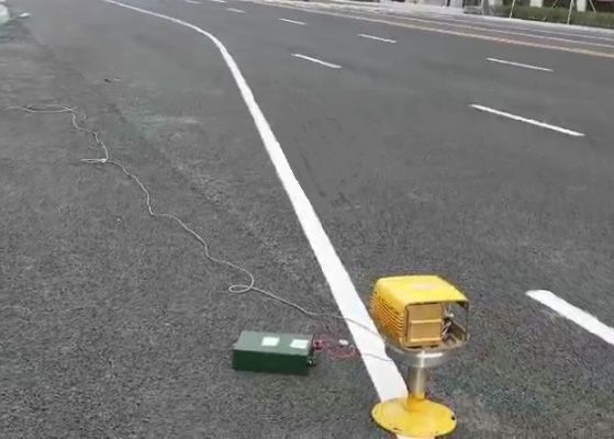
Sensors 2021, 21, 997                                                                                             2 of 19

                        Nevertheless, the detection result still depends on the detection effect of CFAR and is
                        influenced by clutter. Reference [15] established a particle swarm optimization-support
                        vector data description (PSO-SVDD) classifier to detect target signals form ground clutter
                        signals that the classifier parameters were optimized by particle swarm optimization (PSO).
                        For PSO-SVDD classifier, a large number of ground clutter signals are used to train the
                        classifier in the training stage. Compared with the traditional CA-CFAR and CM-CFAR
                        method, this method has a better detection performance. However, the classification
                        boundary is easily overfitted due to lack of target sampling data to train the PSO-SVDD
                        classifier. This paper proposes an improved FOD detection approach based on optimal
                        Variational mode decomposition (VMD) and support vector data description (SVDD). The
                        aims of this method are to suppress ground clutter and improve target detection probability.
                               VMD [16,17], a sparse signal processing method, can decompose a complex signal into
                        an ensemble of band-limited intrinsic mode functions (BLIMFs). The key issue is how to set
                        two crucial parameters of VMD algorithm: the penalty factor α and the decomposition layer
                        number K. In [18,19], the VMD parameters are searched by particle swarm optimization
                        (PSO) algorithm and artificial fish swarm algorithm (AFSA), respectively. From their results,
                        it is feasible to apply artificial intelligence (AI) algorithms for VMD parameter optimization.
                        Whale optimization algorithm (WOA) [20] is an efficient search and optimization method
                        in AI algorithms that has many superiorities, such as fewer input parameters, faster
                        convergence speed, and stronger global search ability. SVDD [21] is one of the most
                        prominent methods for one-class classification that is to find a set containing the most typic
                        instances and rejecting abnormal instances. In this paper, the parameters of VMD are first
                        optimized by WOA. Then radar echo signals are decomposed into FOD intrinsic mode
                        functions (IMFs) and clutter IMFs with the optimal VMD. Finally, clutter IMFs are utilized
                        to train the SVDD classifier, and then targets in FOD IMFs are detected by the trained
                        classifier. Here, the optimal VMD algorithm can not only improve the classification effect
                        of the SVDD classifier but also ensure the stable working performance of the classifier.
                        Experiments are conducted to validate that the proposed VMD-SVDD method can yield
                        preferable detection results in simulation and practical measure.
                               The rest of this paper is organized as follows. In Section 2, the distance measuring prin-
                        ciple of linear frequency modulated continuous wave (LFMCW) radar is introduced. The
                        proposed method is described in detail in Section 3. The Section 4 gives the experimental
                        processes and results. The conclusions are drawn in Section 5.

                        2. Distance Measuring Principle of LFMCW Radar
                              Linear frequency modulated continuous wave (LFMCW) [22] radar is frequently used
                        in radar sensors on airport runways. It is beneficial to detect weak targets under strong
                        ground clutter with LFMCW radar due to the advantages of high range resolution and low
                        transmitting power.
                              Figure 1 is the time-frequency diagram of LFMCW radar. The factors B, T, fT , fR , and
                        f 0 represent the band-width, modulation cycle, sending frequency, receive frequency and
                        center frequency. f b+ and f b− are positive beat frequency and negative beat frequency. τ is
                        time delay. The ranging principle of LFMCW radar is as follows.
                              The frequency of the sending signal is:

                                                                              Bt
                                                                 f T = f0 +                                          (1)
                                                                              T
                             Suppose the target distance is R. The frequency of the received signal is:

                                                                          B      2R
                                                             f R = f0 +     (t −    )                                (2)
                                                                          T       c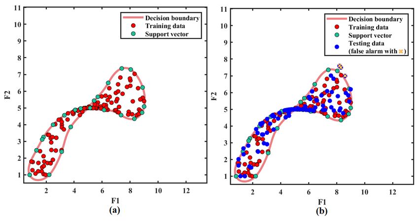
B     2R
                                                                              f R = f0 +        (t − )
                                                                                              T      c
Sensors 2021, 21, 997                                                                                                    3 of 19
                               The light speed is c. The signal delay is τ = 2R c . The beat frequency

                                                                                            2RB
                                                                             f = f The
                               The light speed is c. The signal delay is τ = 2R/c.
                                                                                  b − fbeat
                                                                                         = frequency is:
                                                                                          R     T
                                                                      2RB
                                                                                                     cT
                                                      fb = f R − fT =                              (3)
                         fb   can be calculated by spectrum analysis,  cT and then the target distance R can
                         f b can be calculated by spectrum analysis, and then the target distance R can be obtained.

                         Figure 1. Time-frequency diagram of LFMCW radar.
                        Figure 1. Time-frequency diagram of LFMCW radar.
                             In radar sensors, radar echo signals are mixed with clutter and noise. The noise is
                         mainly the thermal noise in radar receivers, which is much weaker than ground clutter, so
                                In radar
                         it is ignored      sensors,
                                       in this          radar
                                               paper. The        echo signals
                                                          final received signal canare  mixed with
                                                                                    be formulated as: clutter and
                                                                                                     noise.
                        mainly the thermal noises in       radar receivers, which is much weaker(4)than gr
                                                    R ( t ) = s f od ( t ) + sclutter ( t )
                        so it is ignored in this paper. The final received signal can be formulated as:
                         where, s f od (t) is the target signal, and sclutter (t) is the clutter signal. Supposing the sending
                                                                         s (t ) = s (t ) + s
                         signal is s T (t), the signal through the mixer receiver can be expressed as
                                                                              R            fod             (t )
                                                                                                        clutter
                                                                  s(t) = s R (t) × s T (t)                                  (5)
                        where,     s (t)
                             Based fod
                                                is the target signal, and             s
                                                                                clutter
                                   on fast Fourier transform (FFT), it is easy to
                                                                                              (t)   is the clutter signal. Suppos
                                                                                   get the target distance in frequency
                        ing signal is s (t ) , the signal through the mixer receiver can be expressed
                         domain.
                                            T
                                                                                                                                   as
                         3. Proposed Method and Explanation
                              The flowchart of the proposed VMD-SVDD method   s(t) = s (t ) × s (t)
                                                                          R is shown
                                                                                  T in Figure 2. It is de-
                         scribed subsequently in detail.
                           Based on fast Fourier transform (FFT), it is easy to get the target distance
                        domain.

                        3. Proposed Method and Explanation
                             The flowchart of the proposed VMD-SVDD method is shown in Figu
                        scribed subsequently in detail.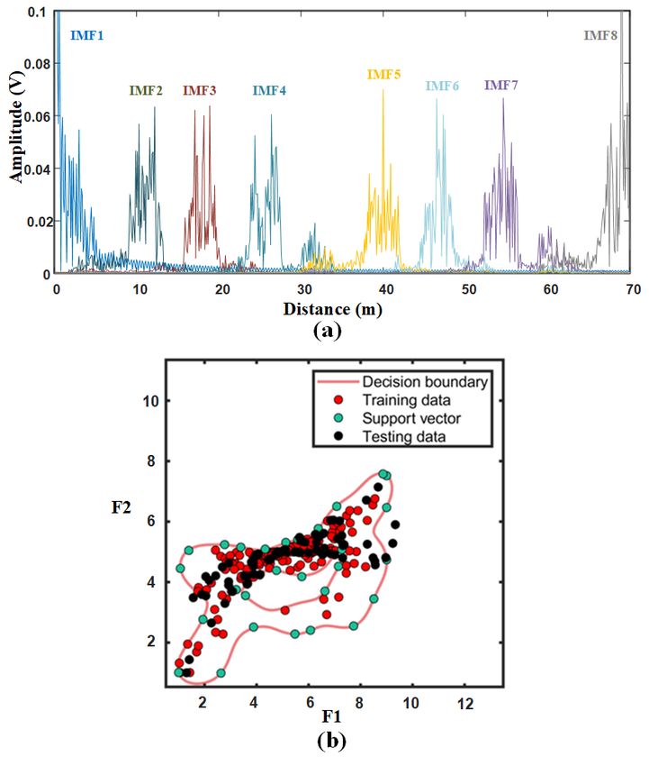
Sensors 2021,2021,
Sensors 21, 21,
997997 4 of 19
Figure
Figure 2. 2. Flowchart
Flowchart of theofproposed
the proposed
method.method.
3.1. VMD Parameter Optimization
3.1. Variational
VMD Parameter Optimization
mode decomposition (VMD) is one of the sparse signal processing methods,
which Variational
was proposedmode in 2014.decomposition
The VMD can (VMD) is oneand
automatically of effectively
the sparsedecompose
signal processin
aods,
complex
which was proposed in 2014. The VMD can automatically and(BLIMFs).
signal into an ensemble of band-limited intrinsic mode functions effectively dec
VMD can be used for filtering and denoising. Compared with other signal decompose
a complex signal into an ensemble of band-limited intrinsic mode functions (B
methods such as empirical modal decomposition (EMD) [23] and ensemble empirical mode
VMD can be(EEMD)
decomposition used [24],
for filtering
VMD overcomes and denoising.
problems of modalCompared aliasing,with othereffect,
end-point signal dec
methods
and such as empirical modal decomposition (EMD) [23] and ensemble e
false component.
modeThedecomposition
VMD is used to decompose
(EEMD)the mixing
[24], VMD signal s(t) into a finite
overcomes number of
problems ofBLIMFs.
modal aliasi
The BLIMF has a central frequency
point effect, and false component. and a limited bandwidth. The constrained variational
model is constructed as follows:
The VMD is used to decompose the mixing signal s (t ) into a finite nu
h i 2
BLIMFs. The
BLIMF
min{hk }has
,{ w k } a ∑
central
K k∂t δfrequency1
(t) + j πt ∗ hand
k (t) ae−limited
jwk t k bandwidth. The con
2
variational model is constructed asK follows: (6)
s.t. ∑ hk = s(t)
k =1
1
2
where { hk } = {h1 , h2 , h3
impulse
−
, .min
. . , hK } is intrinsic mode∂t δ (t ) + j ∗ hk (t ) e
function, ω k = { ω 1 , ω 2 , ω 3 , . . jw
. , t
kωK } is
the center frequency of hk , δ(t){his k },{ wk } unit
π t ∂t is the gradient
the
K
function, and
with
respect to the time series. 2
K
s.t. hk = s(t )
k =1
where {hk } = {h1, h2 ,..., hK } is intrinsic mode function, {wk } = {w1, w2 ,..., wK }
center frequency of hk , δ (t ) is the unit impulse function, and ∂ t is the gradi
respect to the time series.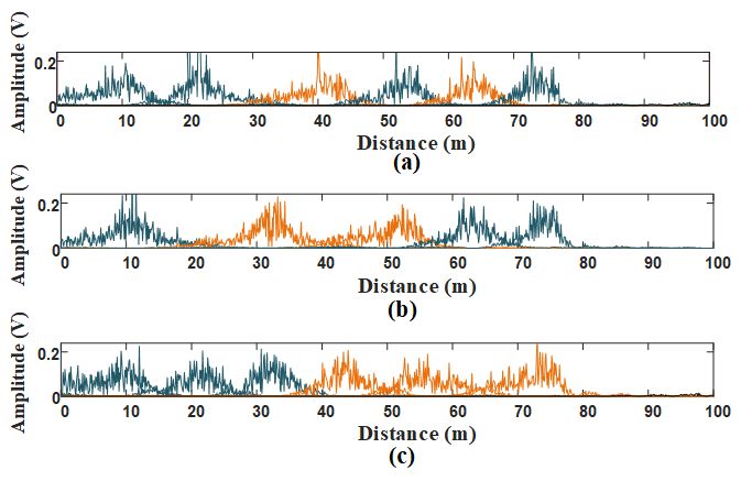
Sensors 2021, 21, 997 5 of 19
To solve the constrained variation problem, quadratic penalty parameter α and
Lagrange operator λ [25] are introduced. The extended Lagrange expression is given
as follows:
2
j 2
L({hk }, {wk }, λ) = α ∗ ∑ k∂t δ(t) + ∗ hk (t) e− jwk t k + ks(t) − ∑ hk (t)k + hλ(t), s(t) − ∑ hk (t)i (7)
K
πt 2 K K
2
By using the alternating direction multiplicative operator method (ADMM) [26], hnk +1 ,
wkn+1 , and λn+1 are updated until the stop condition is satisfied. Among:
2
λ(t) 2
j
n +1
hk (t) = argmin{α ∗ k∂t δ(t) + ∗ hk (t) e− jwk t k + ks(t) − ∑ hk (t) + k } (8)
hk ∈s πt 2 K
2
2
In the VMD processing, penalty factor α and decomposition layer number K need to
be known in advance. The integrity of the decomposed component is determined by α. An
improper K may lead to many problems, such as mode aliasing and false components. The
whale optimization algorithm (WOA) is selected to search suitable α and K for the VMD in
this paper.
Whale optimization algorithm (WOA) is a new heuristic optimization algorithm of
artificial intelligence algorithms, which has advantages of fewer input parameters, faster
convergence speed, and stronger global search ability. The WOA algorithm simulates hunt-
ing behaviors of humpback whales. The mathematical model of WOA can be expressed as:
In a given space, whales will constantly update their positions to get close to the prey
→ →∗
position. That is to say: Give a range of α ∈ [α1 , αn ] and K ∈ [K1 , Km ]. Y i and Y are the
→
whale positions and the prey position respectively. Y i = (α f , K g ), 1 ≤ f ≤ n, 1 ≤ g ≤ m,
→∗ → →∗
1 ≤ i ≤ nm, Y is first given at random. Y i will keep updating to get closer to Y . At the
→∗
same time, Y is kept or updated to the optimal position in each iteration.
There are two whales foraging behaviors, namely, shrinking encircling mechanism
and spiral position updating. The probability of both behaviors is 50%. The model is given
as follows:
→∗ → →
→
Yi − A · D p < 0.5
Y i +1 = ∗ →∗ (9)
→ bl
D · e · cos(2πl ) + Y p ≥ 0.5
i
When p < 0.5:
→ → →∗ →
D = C · Yi − Yi (10)
→ →∗ → →
Y i +1 = Y i − A · D (11)
Among, i is the number of iterations, which is restricted to less than the maximum
→ → → → → → →
number of iterations. A = 2 · a · d − a and C = 2 · d are coefficient vectors, a is linear
→
regressive from 2 to 0, and d is a random vector in [0,1].
When p ≥ 0.5:
→∗ →∗ →
D = Yi − Yi (12)
→ →∗ →∗
Y i+1 = D · ebl · cos(2πl ) + Y i (13)
where b is a constant which determines the logarithmic spiral shape, and l is a random
number in [−1,1].Sensors 2021, 21, 997 6 of 19
In order to strengthen global search ability of WOA, whales also randomly search for
→ → →
the prey. If A ≥ 1, Y i+1 will be updated according to a random whale position Y rand . The
mathematical model is:
→ → → →
D = C · Y rand − Y i (14)
→ → → →
Y i+1 = Y rand − A · D (15)
→∗
During each iteration, the prey position Y always corresponds to the current max-
→∗
imum kurtosis of cross-correlation coefficients between s(t) and hk (t). In the end, Y is
consisted of optimal α and K. Then s(t) is decomposed by VMD with optimal parameters.
Select FOD IMFs and clutter IMFs by the average of cross-correlation coefficients between
s(t) and hk (t).
3.2. SVDD Classification
Support vector data description (SVDD) [27] algorithm is one of the machine learning
algorithms, based on traditional support vector machines (SVM) [28,29]. The SVDD has
been widely applied in anomaly detection, fault detection and diagnosis process. The
basic principle of SVDD is that a minimum hypersphere containing all training samples is
generated in the high-dimensional space. The support vectors are the sample points on
the surface of the hypersphere. Test samples are normal if them are in the hypersphere,
otherwise them are abnormal samples. The training samples (clutter signals in this paper)
are Xt = { xt1 , xt2 , . . . , xt N }. The optimization problem of SVDD can be expressed as
the follows:
2
minB(c, r 0 ) = r 0 + C ∑iN=1 ξ i
2
s.t.( xti − c) T ( xti − c) ≤ r 0 + ξ i (16)
ξ i ≥ 0, ∀i = 1, . . . , N
where C ∑iN=1 ξ i is used to reduce the influence of outliers. ξ i is the slack variable, and
every data point has a corresponding one. When two data points have the same the slack
variable, the hyperspheres are the same. C determines the decision boundary of training
samples. r 0 is the radius. c is the sphere center. The hypersphere can be obtained by using
kernel function [30] and Lagrange multipliers. This paper uses the popular Gaussian kernel
function, which is defined as:
−k xti − xt j k2
K ( xti , xt j ) = exp( ) (17)
σ2
where δ is a parameter that is used to control tightness of the boundary. Gaussian kernel
function provides an efficient technique to map the data of the input space into the high-
dimensional feature space. The dual form of the Equation (16) guided by the Gaussian
kernel function and Lagrange multipliers is:
maxL = ∑in=1 α0 i K ( xti , xt j ) − ∑i,j α0 i α0 j K ( xti , xt j )
s.t.∑in=1 α0 i = 1 (18)
0 ≤ α0 i ≤ C, ∀i = 1, . . . , N
where α0 i corresponds to xti . when α0 i > 0, xti is the support vector. Then the sphere center
c and the radius r 0 can be obtained. The hypersphere is inversely mapped to the original
data space to get the decision boundary of the FOD and clutter.
Before SVDD classification, it is necessary to extract two-dimensional features of
the FOD and clutter as inputs of the classifier. The autocorrelation distribution of FOD
signals is more concentrated while that of ground clutter is more dispersive on account of
target echo signals have stronger correlation than clutter signal. The second-order center
distance (F1) and fourth-order cumulant (F2) of normalized autocorrelation are chosen as
two-dimensional features, which can increase the difference between FODs and clutter. F1Sensors 2021, 21, 997 7 of 19
represents the distribution of normalized autocorrelation relative to the geometric center of
mass. The more dispersed of the distribution is, the smaller F1 is. F2 can further solve the
problems that cannot be solved by F1, such as Gaussian noise. The calculation is as follows:
The normalized autocorrelation coefficient of hk is ri = {r1 , r2 , . . . , rK },
M−h
∑m =1 ( r i m − e
ri )(rim+h − e
ri )
ri = (19)
M
∑m r i )2
=1 ( r i m − e
where M is the length of rim . 0 ≤ h ≤ M. 0 ≤ i ≤ K. eri is the average of rim .
Feature 1: the second order center distance of the normalized autocorrelation coefficient
M
F1 = ∑ e )2 r i m
(m − m (20)
m =1
M M
e = ∑m
where m =1 m ∗ p m , p m = r i m / ∑ m =1 r i m .
Feature 2: fourth-order cumulant of normalized autocorrelation coefficient
M M 2
F2 = ∑ e )4 r i m − 3[ ∑ ( m − m
(m − m e )2 r i m ] (21)
m =1 m =1
4. Discussion
The operation and signal processing parameters of the radar system are provided in
Table 1. The carrier frequency is 96 GHz, and the modulation signal is the linear frequency
modulated signal with the bandwidth of 1.5 GHz. The polarization is VV. Radar antenna
beam width should be as small as possible to obtain better resolution of transverse range.
In this paper, the horizontal beam width is 1.9◦ , the pitch beam width is 5◦ , and the range
resolution is 0.1 ms. The angular step is 12◦ /s, so the maximum pulse accumulation time
is calculated to be 158 ms. The paper adopts the cumulative time of 60 ms, according to
the actual target detection strategy and the transmission between upper computer and
radar sensor.
Table 1. Parameters of the LFMCW radar system.
Parameter Value Parameter Value
bandwidth 1.5 GHz antenna gain 20 dBi
sampling frequency 20 MHz horizontal beam width 1.9◦
farthest monitoring distance 70 m pitch beam width 5◦
range resolution 0.1 m beam width in azimuth 120◦
FFT point number 1024 beam width in downward 28◦
frequency modulation cycle 128 us angular step 12◦ /s
pulse accumulation number 468 cumulative time 60 ms
4.1. Signal Decomposition and Mode Selection
In the simulation, the ground clutter signal is the signal whose amplitude distribution
satisfies Rayleigh distribution, and the target signal is linear frequency modulation signal.
Suppose that there is a target at a distance of 40 m, which is marked with red star in the
following figures. Without clutter signals, the target signal is obvious after frequency
mixing and fast Fourier transform (FFT) processing that shown in Figure 3a. When the
signal-to-clutter rate (SCR) is −20 dB, the target signal almost hides in clutter signals in
Figure 3b. It can be seen that the target at 40 m is obscured by the surrounding strong
clutter in the amplitude spectrum. At this point, it is difficult to detect the target with the
ordinary CFAR method.in the following figures. Without clutter signals, the target signal is obvious after fre-
quency mixing and fast Fourier transform (FFT) processing that shown in Figure 3a. When
the signal-to-clutter rate (SCR) is −20 dB, the target signal almost hides in clutter signals
in Figure 3b. It can be seen that the target at 40 m is obscured by the surrounding strong
Sensors 2021, 21, 997 8 of 19
clutter in the amplitude spectrum. At this point, it is difficult to detect the target with the
ordinary CFAR method.
Figure 3. Simulation data: (a) Target signals without clutter; (b) Target signals with clutter.
Figure 3. Simulation data: (a) Target signals without clutter; (b) Target signals with clutter.
In the proposed method, firstly, quadratic penalty parameter α and decomposition
In the
layer proposed
number method, firstly,
K of variational mode quadratic
decompositionpenalty parameter
(VMD) need to be α searched
and decomposition
by whale
layer number K
optimization algorithm (WOA). In the experiment, the initial rangestoofbeα searched
of variational mode decomposition (VMD) need and K areby
whale optimization
and [5, algorithm
10]. The fitness (WOA).
function In thefunction)
(objective experiment, themaximum
is the initial ranges of αof and
kurtosis cross-K
arecorrelation
[1000, 2000] and [5, 10].
coefficients The fitness
between function
s(t) and hk (t) of(objective
the updatingfunction)
VMD. Theis the maximum
maximum kur-
itera-
tosis
tionofiscross-correlation
15. The parametercoefficients process ofs (WOA
optimizationbetween t ) and hk (t ) in
is shown ofFigure
the updating VMD. The
4. The maximum
Sensors 2021, 21, 997 kurtosis appears
maximum iterationafter 11.iterations.
is 15 At thisoptimization
The parameter time, the optimal
processparameters
of WOAsearched
is shownbyinthe
9Fig-
of 19
WOA are K = 7.69 and α = 1497.10, and the integer formats of them are K
ure 4. The maximum kurtosis appears after 11 iterations. At this time, the optimal param- = 7 and α = 1500,
which are provided for the VMD.
eters searched by the WOA are K = 7.69 and α = 1497.10, and the integer formats of them
are K = 7 and α = 1500, which are provided for the VMD.
Figure 4. Optimization process of the WOA.
Figure 4. Optimization process of the WOA.
Then, the signals in Figure 3b are decomposed by the optimal VMD. The result is
shownThen, the signals
in Figure 5. Theseinmodes
Figureare
3bdistributed
are decomposed
from lowby the optimal
frequency VMD.
to high The result
frequency. The is
shown inassigned
target is Figure 5.toThese modes
the IMF3, andare distributed
clutter from
signals are low frequency
divided into otherto highItfrequency.
IMFs. can be
seentarget
The form is
theassigned
IMF3 that tothe
theclutter
IMF3,signals around
and clutter the target
signals is reduced.
are divided into other IMFs. It can
be seen form the IMF3 that the clutter signals around the target is reduced.Figure 4. Optimization process of the WOA.
Then, the signals in Figure 3b are decomposed by the optimal VMD. The r
shown in Figure 5. These modes are distributed from low frequency to high freq
Sensors 2021, 21, 997 The target is assigned to the IMF3, and clutter signals are divided into9 other
of 19 IMFs
be seen form the IMF3 that the clutter signals around the target is reduced.
Figure 5. Signal decomposition using the optimal VMD.
Figure 5. Signal decomposition using the optimal VMD.
To select FOD mode component, set a selection threshold which is the average of
cross-correlation coefficients of s(t) and hk (t). The first IMF has no value by analyzing
measured data and the last IMF is the residual, these two modes are discarded in the
threshold estimation. The threshold value is calculated as follows:
∑in=1 (si − e
s)(hki − e
hk )
Corrk = q , k = 2, 3, . . . , K − 1 (22)
2
s)2 ∑in=1 (hki − e
∑in=1 (si − e hk )
1
Tcorr = (Corr2 + Corr3 + . . . + CorrK−1 ) (23)
5
n is the length of s(t) and hk (t). e
s is the average of s(t). e
hk is the average of hk (t).
Figure 6 shows the mode selection result of modes in Figure 5, and the red dotted
line is the threshold. The mode whose cross-correlation coefficient exceeds the threshold is
selected as FOD mode component; otherwise, it is classified as clutter mode component.
The cross-correlation coefficient of the mode component including targets is bigger due to
target echo signals have stronger correlation than clutter signals. Here, IMF3 and IMF5
are FOD mode components, and IMF2, IMF4 and IMF6 are clutter mode components. The
IMF1 includes strong clutter signals near radar sensor, which will improve the threshold
value of mode selection. So, it will be discarded in the later signal processing.hk ( t ) .
Figure 6 shows the mode selection result of modes in Figure 5, and the red dotted
line is the threshold. The mode whose cross-correlation coefficient exceeds the threshold
is selected as FOD mode component; otherwise, it is classified as clutter mode component.
The cross-correlation coefficient of the mode component including targets is bigger due
to target echo signals have stronger correlation than clutter signals. Here, IMF3 and IMF5
Sensors 2021, 21, 997 are FOD mode components, and IMF2, IMF4 and IMF6 are clutter mode components. The 10 of 19
IMF1 includes strong clutter signals near radar sensor, which will improve the threshold
value of mode selection. So, it will be discarded in the later signal processing.
Figure 6. IMF selection with the cross-correlation threshold.
Figure 6. IMF selection with the cross-correlation threshold.
In addition,
In addition, the following
the following experimentsexperiments have been
have been conducted conducted
to illustrate the im- to illustrate the impor-
portance of setting
tance of settingappropriate VMD parameters
appropriate and the cross-correlation
VMD parameters threshold.
and the cross-correlation threshold.
The simulation data in Figure 3b is decomposed by VMD with different penalty fac-
The simulation data in Figure 3b is decomposed by
tor α and decomposition layer number K . These mode components are shown in Fig-VMD with different penalty factor
and decomposition layer number K. These mode components
ure 7. The yellow parts are selected as target modes by the cross-correlation threshold.
α are shown in Figure 7. The
Compared with the results in Figure 7b,c, the target signal at 40 m in Figure 7a is
yellow parts are selected as target modes by the cross-correlation threshold. Compared intact
Sensors 2021, 21, 997 when VMD parameters are α = 2000 and K = 7. In Figure 7b, α = 2000 and K = 5. The 11 of 19
with the results in Figure 7b,c, the target signal at 40 m in Figure 7a is intact when VMD
parameters are α = 2000 and K = 7. In Figure 7b, α = 2000 and K = 5. The inaccurate
decomposition is caused by improper K, bringing false components. In Figure 7c, α = 1000
inaccurate decomposition is caused by improper K , bringing false components. In Fig-
K =7c,
and ure 7. αThe integrity
= 1000 and K =of 7. target signalofistarget
The integrity destroyed
signal by the inappropriate
is destroyed α. In Figure 7b,c,
by the inappropriate
the target
α. In Figures 7b,c, the target signals in selected target modes are weaken, which areundetectable
signals in selected target modes are weaken, which are almost almost in
the next signal processing. Therefore, it is necessary to optimize VMD parameters
undetectable in the next signal processing. Therefore, it is necessary to optimize VMD by WOA,
whichparameters
ensures bytheWOA, whichof
integrity ensures
targetthe integrity of target signals.
signals.
VDM 7.processing
Figure 7. Figure with different parameters: (a) VMD parameters are α = 2000 and K = 7; (b) VMD parameters
VDM processing with different parameters: (a) VMD parameters are α = 2000 and K = 7 ; (b) VMD parame-
are α = 2000 andαK==
ters are 5; (c)
2000 andVMDK = parameters are α = 1000
5 ; (c) VMD parameters are αand K =and
= 1000 7. K = 7 .
Figure 8 shows the results of mode selection based on the the cross-correlation
threshold in four cases. There is a target 40 m form the radar sensor in Figure 8a,c. And
there are two targets in Figures 8b,d: one is 25 m from the radar sensor, the other is 55 m
from the radar sensor. The SCR is −15 dB in Figure 8a,b, and the SCR is −20 dB in Figures
8c,d. In Figure 8, the abscissa is the serial number of the mode, the y-coordinate is the
cross-correlation coefficient, and the red dotted line is the threshold.Sensors 2021, 21, 997 11 of 19
Figure 8 shows the results of mode selection based on the the cross-correlation thresh-
old in four cases. There is a target 40 m form the radar sensor in Figure 8a,c. And there are
two targets in Figure 8b,d: one is 25 m from the radar sensor, the other is 55 m from the radar
Sensors 2021, 21, 997 sensor. The SCR is −15 dB in Figure 8a,b, and the SCR is −20 dB in Figure 8c,d. In Figure 8, 12 of 19
the abscissa is the serial number of the mode, the y-coordinate is the cross-correlation
coefficient, and the red dotted line is the threshold.
Figure 8. Mode selection results in four cases: (a) Single target with SCR = −15 dB; (b) Two targets
Figure 8. Mode selection results in four cases: (a) Single target with SCR = −15 dB ; (b) Two tar-
with SCR = −15 dB; (c) Single target with SCR = −20 dB; (d) Two targets with SCR = −20 dB.
gets with SCR = −15 dB ; (c) Single target with SCR = −20 dB ; (d) Two targets with
SCR It= −can
20 dB .
be seen from these selection results that, with the decrease of signal-to-clutter
rate (SCR), the number of modes below the threshold decreases and the selected clutter
modes
4.2. SVDDdecrease, regardless
Classification of Fod
and single target or multiple targets. From the above simulation
Detection
results, the number of clutter data used to train the classifier is sufficient, although some of
After the mode components are divided into FOD modes and clutter modes by the
clutter modes are selected as target modes. Moreover, if the number of targets increases
cross-correlation threshold, the SVDD classifier is used to distinguish FOD signals from
further, more clutter modes can be obtained by increasing the decomposition layer of VMD.
clutter
But thissignals.
case of too many targets on airport runways is not common.
In the simulation, two important parameters of SVDD are set as follows: δ = 0.5 and
4.2.
C SVDD
= 1, which Classification and Fod
are optimized by Detection
particle swarm optimization (PSO) [15]. According to Equa-
tion (20) and Equation (21), feature
After the mode components are divided vectorsinto
of FOD
the training
modes andsamples
clutter(clutter
modes bysignals)
the are
obtained to trainthreshold,
cross-correlation SVDD classifier.
the SVDD classifier is used to distinguish FOD signals from
clutter signals.VMD processing, after the SVDD classifier is trained by clutter signals in the
Without
FigureIn 3b,
the the
simulation, two important
red optimal parametersisofobtained
decision boundary SVDD areas set as follows:
shown δ = 9a.
in Figure 0.5 In the
and C = 1, which are optimized by particle swarm optimization (PSO) [15]. According
training stage, the optimal decision boundary is obtained. In the testing stage, if sampling to
Equations (20) and (21), feature vectors of the training samples (clutter signals) are obtained
points falls within the boundary, they are considered as clutter signals. Otherwise, they
to train SVDD classifier.
will be considered as non-clutter signals. The simulation data from Figure 3b are tested
by the trained SVDD classifier. The classification result is shown in Figure 9b. The sam-
pling points outside the boundary are false alarms, which are marked with yellow cross
in figures. The sampling points of the target can hardly be found due to the effect of strong
clutter.
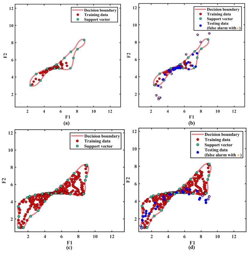
With VMD processing, the clutter modes in Figure 5 are selected to train the classifierSensors 2021, 21, 997 12 of 19
Without VMD processing, after the SVDD classifier is trained by clutter signals in the
Figure 3b, the red optimal decision boundary is obtained as shown in Figure 9a. In the
Sensors 2021, 21, 997 training stage, the optimal decision boundary is obtained. In the testing stage, if sampling 13 of 19
points falls within the boundary, they are considered as clutter signals. Otherwise, they will
be considered as non-clutter signals. The simulation data from Figure 3b are tested by the
trained SVDD classifier. The classification result is shown in Figure 9b. The sampling points
seen fromthe
outside above experiments,
boundary VMD processing
are false alarms, can reduce
which are marked the effect
with yellow crossofinclutter
figures.on target
The
signals, which improves the SVDD classification efficiency.
sampling points of the target can hardly be found due to the effect of strong clutter.
Figure
Figure 9. Classification
9. Classification results:
results: (a)(a) Trainingresult
Training resultwithout
without VMD
VMD processing;
processing;(b)
(b)Testing
Testingresult without
result VMD
without processing;
VMD processing;
(c) Training result with VMD processing; (d) Testing result with VMD
(c) Training result with VMD processing; (d) Testing result with VMD processing.processing.
In order to test the classification performance of VMD-SVDD classifier, the proposed
method is tested on a clutter data set without targets. In this case, the cross-correlation
mode selection algorithm will mistakenly select some of the clutter modes as the target
modes (called false target modes). However, sampling points of these false target modes
are likely to be classified into the decision boundary by the trained classifier. As can beSensors 2021, 21, 997 13 of 19
With VMD processing, the clutter modes in Figure 5 are selected to train the classifier
and the FOD modes are tested by the trained VMD-SVDD classifier. Figure 9c shows the
training result and Figure 9d shows the testing result. Although there are still some false
alarms outside the decision boundary, some sampling points of the target can be detected.
Here, a target corresponds to multiple sampling points in the figure due to radar signals
are linear frequency modulated continuous wave signals. By Comparing the results in
Figure 9b,d, it is easier to detect targets in Figure 9d under the same SCR. As can be seen
Sensors 2021, 21, 997 from above experiments, VMD processing can reduce the effect of clutter on target signals,
14 of 19
which improves the SVDD classification efficiency.
In order to test the classification performance of VMD-SVDD classifier, the proposed
method is tested on a clutter data set without targets. In this case, the cross-correlation
For the training of VMD-SVDD classifier, the training set includes clutter modes se-
mode selection algorithm will mistakenly select some of the clutter modes as the target
lected by the cross-correlation threshold after VMD processing. While, the testing set in-
modes (called false target modes). However, sampling points of these false target modes
cludes target modes, and may also include other clutter modes. From above simulation
are likely to be classified into the decision boundary by the trained classifier. As can be
and test results, it can be seen that using clutter modes as a test set results in an error
seen from Figure 10, false alarms appear very close to the decision boundary. After a large
probability of about 0.8% , which has little effect on target detection. So, the training way
number of repeated experiments, it is found that the false alarm probability of the proposed
of the VMD-SVDD classifier proposed in this paper is reliable.
method is about 0.8%.
Figure 10.
Figure Classification results
10. Classification results of
of clutter
clutter data
data set:
set: (a)
(a) Training
Training result;
result; (b)
(b) Testing
Testing result.
result.
For the training of VMD-SVDD classifier, the training set includes clutter modes
To compare the detection performance of the proposed VMD-SVDD method, four
selected by the cross-correlation threshold after VMD processing. While, the testing set
methods are applied to detect a same target under different SCR. The cell-average CFAR
includes target modes, and may also include other clutter modes. From above simulation
(CA-CFAR) method is to obtain a detection threshold by averaging the clutter power
and test results, it can be seen that using clutter modes as a test set results in an error
around the target. If the amplitude of a signal exceeds the threshold, the signal is consid-
probability of about 0.8%, which has little effect on target detection. So, the training way of
ered as a target. The
the VMD-SVDD principle
classifier of VMD-CACFAR
proposed in this papermethod is to detect targets in FOD mode
is reliable.
components
To compare the detection performance of the proposed the
by CA-CFAR method. In SVDD method and proposed method,
VMD-SVDD VMD-SVDDfour
method, target sampling points are marked in advance, and the target is
methods are applied to detect a same target under different SCR. The cell-average CFARdetected by con-
firming that sampling points outside the decision boundary are labeled.
(CA-CFAR) method is to obtain a detection threshold by averaging the clutter power around
The numbers
the target. of simulation
If the amplitude of aare 1000 exceeds
signal in everythecasethreshold,
and the detection probability
the signal ( Pd )
is considered
result is shown
as a target. The in Figure of
principle 11.VMD-CACFAR
Under differentmethodSCR, P isd toofdetect
the proposed
targets inVMD-SVDD
FOD mode
components by CA-CFAR method. In SVDD method and the proposed
method is higher than that of other methods. Especially, the target can almost always be VMD-SVDD
method, target
accurately sampling
detected when SCRpoints are dB.
> −10 marked
It caninbeadvance,
seen from and the target
Figure 10 thatisthe
detected by
detection
confirming that sampling points outside the decision boundary are
performance based on SVDD or VMD-SVDD is better than that based on CA-CFAR or labeled.
VMD-CACFAR. Compared with the SVDD classifier, the proposed VMD-SVDD classifier
has the higher detection probability, which proves that the optimal VMD can improve the
accuracy of SVDD classification.
Then the real-time analysis of above four methods is carried out, and the time re-
quired to run these algorithms is shown in Table 2. Among them, the running time of theSensors 2021, 21, 997 14 of 19
The numbers of simulation are 1000 in every case and the detection probability (Pd )
result is shown in Figure 11. Under different SCR, Pd of the proposed VMD-SVDD method
is higher than that of other methods. Especially, the target can almost always be accurately
detected when SCR > −10 dB. It can be seen from Figure 10 that the detection performance
based on SVDD or VMD-SVDD is better than that based on CA-CFAR or VMD-CACFAR.
Sensors 2021, 21, 997 Compared with the SVDD classifier, the proposed VMD-SVDD classifier has the higher 15 of 19
detection probability, which proves that the optimal VMD can improve the accuracy of
SVDD classification.
Figure 11. Detection probabilities of four detection methods.
Figure 11. Detection probabilities of four detection methods.
Then the real-time analysis of above four methods is carried out, and the time required
Table
to run2.these
Real-time analysis
algorithms of four
is shown inmethods.
Table 2. Among them, the running time of the proposed
algorithm is
Method 10.93 s, which is
CA-CFAR acceptable inVMD-CACFAR
actual projects. By comparing
SVDD theVMD-SVDD
running
time and detection probability of above four detection methods, it can be seen that while
Run time (s) 0.25 9.87 4.91 10.93
the detection probability of the proposed method is high, the running time is long. In
particular, VMD algorithm increased running time. In future work, the VMD module can
4.3. Field Measure
be optimized and Validation
to improve Result
the run time of the proposed method.
To verify general validity of the proposed VMD-SVDD method, it is applied to a ra-
Table
dar 2. Real-time
sensor systemanalysis of four methods.
in reality. Figure 12
is the photograph of field measure scenario. Two
cases Method
were tested in CA-CFAR
this field: in VMD-CACFAR
scene 1, a metal ballSVDD
was placed VMD-SVDD
40 m from the radar
sensor; in scene 2, two bolts
Run time (s) 0.25
were placed 40 m and 55 m4.91
9.87
from the radar10.93
sensor. The radar
echo signals are processed by the proposed VMD-SVDD method.
4.3. Field Measure and Validation Result
To verify general validity of the proposed VMD-SVDD method, it is applied to a radar
sensor system in reality. Figure 12 is the photograph of field measure scenario. Two cases
were tested in this field: in scene 1, a metal ball was placed 40 m from the radar sensor; in
scene 2, two bolts were placed 40 m and 55 m from the radar sensor. The radar echo signals
are processed by the proposed VMD-SVDD method.To verify general validity of the proposed VMD-SVDD met
dar sensor system in reality. Figure 12 is the photograph of field
cases were tested in this field: in scene 1, a metal ball was plac
Sensors 2021, 21, 997 sensor; in scene 2, two bolts were placed 40 m and 55 m from
15 of 19 the
echo signals are processed by the proposed VMD-SVDD method
Figure
Figure12. Field
12. measure scenario.
Field measure scenario.
For scene 1, the original signal after frequency mixing and FFT processing is shown in
Figure 13a. As can be seen that the signal of the metal ball 40 m from the radar sensor is
For scene 1, the original signal after frequency mixing and
obscured by surrounding strong clutter signals. After the proposed method processing, the
Sensors 2021, 21, 997 16 of 19
in Figure
detection result 13a. Asin can
is shown Figurebe13bseen
that thethat
target the
signalsignal of thewith
can be detected metal ball
two false 40
alarms existing around the target. The problem of false alarms will be discussed later.
is obscured by surrounding strong clutter signals. After the prop
the detection result is shown in Figure 13b that the target signal c
false alarms existing around the target. The problem of false alarm
Figure 13. Signals in scene 1: (a) Original signal; (b) Target detection result.
Figure 13. Signals in scene 1: (a) Original signal; (b) Target detection result.
Figure 14a shows mode components after VMD processing of scene 1. Where, IMF2,
Figure
IMF3, IMF6 14a shows
and IMF7 mode components
are selected as clutterafter
modes VMD processing
to train the SVDDofclassifier,
scene 1.andWhere,
targetIMF2,
IMF3, IMF6
modes areand
IMF4IMF7and are selected
IMF5. as clutter
Through modes
analysis of thetomeasured
train the data,
SVDD theclassifier,
first IMFand
andtarget
the last
modes areIMF
IMF4have
and a great
IMF5.influence
Throughonanalysis
the finalofselection result. Therefore,
the measured both IMF
data, the first modesand the
are discarded in the selection threshold estimation, which is the same as
last IMF have a great influence on the final selection result. Therefore, both modes are the simulation.
According to the actual situation, the decomposition layer number K of VMD is adaptively
discarded in the selection threshold estimation, which is the same as the simulation. Ac-
cording to the actual situation, the decomposition layer number K of VMD is adaptively
adjusted to 8 . The SVDD classification result is shown in Figure 14b. The sampling points
outside the decision boundary belongs to the target or false alarm.
Here, both Figures 13b and 14b show the detection result of single target. Figure 13bSensors 2021, 21, 997 16 of 19
Sensors 2021, 21, 997 17
adjusted to 8. The SVDD classification result is shown in Figure 14b. The sampling points
outside the decision boundary belongs to the target or false alarm.
Figure 14. Signal processing for scene 1: (a) Mode components after VMD processing; (b) SVDD
Figure 14. Signal processing for scene 1: (a) Mode components after VMD processing; (b)SVDD
classification result.
classification result.
Here, both Figures 13b and 14b show the detection result of single target. Figure 13b
represents the result in the distance dimension, while Figure 14b represents the result in
the feature space. For scene 1, the final detection result is that two false alarms appear
around the single target, so there are three lines in Figure 13b, corresponding to three points
outside the decision boundary in Figure 14b.
For scene 2, the original signal is shown as Figure 15a,b shows the detection result
that both targets are correctly detected. There are still false alarms around the target 40 m
from the radar sensor.Sensors 2021, 21, 997 17 of 19
Figure 14. Signal processing for scene 1: (a) Mode components after VMD processing; (b)SVDD
classification result.
Figure 15. Signals in scene 2: (a) Original signal; (b) Target detection result.
Figure 15. Signals in scene 2: (a) Original signal; (b) Target detection result.
In fact, if false alarm objects are very close to the target, it has little impact on the
detection result. In the future work, how to improve the detecting probability of such
5. Conclusions
situation will be further researched.
The FOD detection method in the MMW radar sensor system is limited by the stro
ground clutter on the airport runway. This work presents an improved VMD-SVD
5. Conclusions
The FOD detection method in the MMW radar sensor system is limited by the strong
ground clutter on the airport runway. This work presents an improved VMD-SVDD method
to detect FODs. In this method, the echo signal received by MMW radar system are is firstly
decomposed into BLIMFs with the optimal VMD. Then the mode components divided
into two parts: FOD mode components and clutter components. The selected clutter mode
components are used to train the SVDD classifier, and then the FOD mode components
are tested by the classifier. This method relies on the SVDD classifier to distinguish FOD
signals from clutter signals, what’s more, the accuracy and stability of the classifier is
improved by the optimal VMD. The proposed method has two significant advantages:
(1) The VMD-SVDD method is more adaptable. There is no need to set VMD parameters,
among which quadratic penalty parameter α and decomposition layer number K are
searched by the WOA algorithm;
(2) The VMD-SVDD method can effectively suppress ground clutter signals and has the
higher detection probability.
After analytically describing the procedure, the effectiveness of the approach has been
proven by simulation. Furthermore, the general validity of the method is evidenced with
the measured data.
Author Contributions: Conceptualization, J.Z. and X.G.; methodology, J.Z., Q.S. and X.G.; software,
X.G.; formal analysis, Q.S.; investigation, X.L. and Q.Z.; writing—original draft preparation, J.Z.
and X.G.; writing review and editing, Q.S., X.L. and Q.Z. All authors have read and agreed to the
published version of the manuscript.
Funding: This research was funded by National Natural Science Foundation of China, grant
number 61901288.
Institutional Review Board Statement: Not applicable.Sensors 2021, 21, 997 18 of 19
Informed Consent Statement: Not applicable.
Data Availability Statement: The data presented in this study are available on request from the
corresponding author. The data are not publicly available due to privacy.
Conflicts of Interest: The authors declare no conflict of interest.
References
1. Yonemoto, N.; Kohmura, A.; Futatsumori, S.; Uebo, T.; Saillard, A. Broad band RF module of millimeter wave radar network
for airport FOD detection system. In Proceedings of the 2009 International Radar Conference “Surveillance for a Safer World”,
Bordeaux, France, 12–16 October 2009; pp. 1–4.
2. Tarsier®: Automatic Runway FOD Detection System. Available online: https://www.tarsierfod.com/ (accessed on 19 December 2018).
3. What Is FODetect? Available online: http://www.xsightsys.com/fodetect.html (accessed on 24 January 2018).
4. FOD Finder™. Available online: https://www.xsightsys.com/index.php/fodetect/ (accessed on 4 January 2016).
5. Zeitler, A.; Lanteri, J.; Pichot, C. Folded Reflectarrays With Shaped Beam Pattern for Foreign Object Debris Detection on Runways.
IEEE Trans. Antennas Propag. 2010, 58, 3065–3068. [CrossRef]
6. Futatsumori, S.; Morioka, K.; Kohmura, A. Design and Field Feasibility Evaluation of Distributed-Type 96 GHz FMCW Millimeter-
Wave Radar Based on Radio-Over-Fiber and Optical Frequency Multiplier. J. Light. Technol. 2016, 34, 4835–4843. [CrossRef]
7. Baoshuai, W.; Jianghong, L.; Xiaoliang, Z. A novel hierarchical foreign obeject debris detection method for millimeter wave radar.
In Proceedings of the International Applied Computational Electromagnetics Society Symposium ACES IEEE, Firenze, Italy,
26–30 March 2017.
8. Galati, G.; Ferri, M.; Marti, F. Advanced radar techniques for the air transport system: The surface movement miniradar concept.
In Proceedings of the IEEE National Telesystems Conference, San Diego, CA, USA, 26–28 May 1994; pp. 331–338.
9. Galati, G.; Leonardi, M.; Cavallin, A.; Pavan, G. Airport Surveillance Processing Chain for High Resolution Radar. IEEE Trans.
Aero Elect. Syst. 2010, 46, 1522–1533. [CrossRef]
10. Yang, X.; Huo, K.; Zhang, X. A Clutter-Analysis-Based STAP for Moving FOD Detection on Runways. Sensors 2019, 19, 549.
[CrossRef]
11. Moustafa, A.; Ahmed, F.M.; Moustafa, K.H.; Halwagy, Y. A new CFAR processor based on guard cells information. In Proceedings
of the IEEE Radar Conference, Atlanta, GA, USA, 7–11 May 2012; pp. 133–137. [CrossRef]
12. Xiaoqi, Y. An Anti-FOD Method Based on CA-CM-CFAR for MMW Radar in Complex Clutter Background. Sensors 2020, 20, 1635.
[CrossRef]
13. Conte, E.; Longo, M.; Lops, M. Modelling and simulation of non-Rayleigh radar clutter. IEE Proc. F Radar Signal Process. 1991, 138,
121–130. [CrossRef]
14. Baoshuai, W.; Minjue, H.; Jianghong, L.; Xiaoliang, Z. A Hierarchical FOD Detection Scheme Based on Clutter Map CFAR
and Pattern Classification. In Proceedings of the IEEE International Conference on Signal Processing, Communications and
Computing ICSPCC, Qingdao, China, 14–17 September 2018; pp. 1–6.
15. Ni, P.; Miao, C.; Tang, H. Small Foreign Object Debris Detection for Millimeter-Wave Radar Based on Power Spectrum Features.
Sensors 2020, 20, 2316. [CrossRef] [PubMed]
16. Dragomiretskiy, K.; Zosso, D. Variational Mode Decomposition. IEEE Trans. Signal Process. 2014, 62, 531–544. [CrossRef]
17. Gok, G.; Alp, Y.K.; Altıparmak, F. Radar fingerprint extraction via variational mode decomposition. In Proceedings of the 25th
Signal Processing and Communications Applications Conference SIU, Antalya, Turkey, 15–18 May 2017; pp. 1–4. [CrossRef]
18. Long, J.; Wang, X.; Dai, D.; Tian, M.; Zhu, G.; Zhang, J. Denoising of UHF PD signals based on optimised VMD and wavelet
transform. IET Sci. Meas. Technol. 2017, 11, 753–760. [CrossRef]
19. Li, H.; Chang, J.; Xu, F.; Liu, Z.; Yang, Z.; Zhang, L.; Zhang, S.; Mao, R.; Dou, X.; Liu, B. Efficient Lidar Signal Denoising Algorithm
Using Variational Mode Decomposition Combined with a Whale Optimization Algorithm. Remote Sens. 2019, 11, 126. [CrossRef]
20. Zhang, Q.; Liu, L. Whale Optimization Algorithm Based on Lamarckian Learning for Global Optimization Problems. IEEE Access
2019, 7, 36642–36666. [CrossRef]
21. Görnitz, N.; Lima, L.A.; Müller, K.; Kloft, M.; Nakajima, S. Support Vector Data Descriptions and k-Means Clustering: One Class.
IEEE Trans. Neural Netw. Learn. Syst. 2017, 29, 3994–4006. [CrossRef] [PubMed]
22. Geroleo, F.G.; Brandt-Pearce, M.; Brown, C.L. Detection and estimation of multi-pulse LFMCW radar signals. In Proceedings of
the IEEE Radar Conference, Washington, DC, USA, 10–14 May 2010; pp. 1009–1013.
23. Rilling, G.; Flandrin, P. One or two frequencies: The empirical mode decomposition answers. IEEE Trans. Signal. Process. 2008,
56, 85–95. [CrossRef]
24. Chan, J.; Ma, H.; Saha, T.; Ekanayake, C. Self-adaptive partial discharge signal de-noising based on ensemble empirical mode
decomposition and automatic morphological thresholding. IEEE Trans. Dielectr. Electr. Insul. 2014, 21, 294–303. [CrossRef]
25. David, S.A.; Valentim, C.A., Jr. Fractional Euler-Lagrange Equations Applied to Oscillatory Systems. Mathematics 2015, 3, 258–272.
[CrossRef]
26. Xie, D.; Esmaiel, H.; Sun, H.; Qi, J.; Qasem, Z.A.H. Feature Extraction of Ship-Radiated Noise Based on Enhanced Variational
Mode Decomposition, Normalized Correlation Coefficient and Permutation Entropy. Entropy 2020, 22, 468. [CrossRef] [PubMed]Sensors 2021, 21, 997 19 of 19
27. Huan, Z.; Wei, C.; Li, G.H. Outlier Detection in Wireless Sensor Networks Using Model Selection-Based Support Vector Data
Descriptions. Sensors 2018, 18, 4328. [CrossRef] [PubMed]
28. Keerthi, S.S. Efficient tuning of SVM hyperparameters using radius/margin bound and iterative algorithms. IEEE Trans. Neural
Netw. 2002, 13, 1225–1229. [CrossRef] [PubMed]
29. Balasundaram, S.; Kapil, N. Application of Lagrangian Twin Support Vector Machines for Classification. In Proceedings of
the 2nd International Conference on Machine Learning and Computing, Bangalore, India, 9–11 February 2010; pp. 193–197.
[CrossRef]
30. Munoz-Marf, J.; Bruzzone, L.; Camps-Vails, G. A support vector domain description approach to supervised classifification of
remote sensing images. IEEE Trans. Geosci. Remote Sens. 2007, 45, 2683–2692. [CrossRef]You can also read