New correction method for the scattering coefficient measurements of a three-wavelength nephelometer
←
→
Page content transcription
If your browser does not render page correctly, please read the page content below
Atmos. Meas. Tech., 14, 4879–4891, 2021
https://doi.org/10.5194/amt-14-4879-2021
© Author(s) 2021. This work is distributed under
the Creative Commons Attribution 4.0 License.

New correction method for the scattering coefficient measurements
of a three-wavelength nephelometer
Jie Qiu1 , Wangshu Tan1,2 , Gang Zhao1,3 , Yingli Yu4,1 , and Chunsheng Zhao1
1 Department  of Atmospheric and Oceanic Sciences, School of Physics, Peking University, Beijing 100871, China
2 School of Optics and Photonics, Beijing Institute of Technology, Beijing 100081, China
3 State Key Joint Laboratory of Environmental Simulation and Pollution Control, College of Environmental Sciences and

Engineering, Peking University, Beijing 100871, China
4 Economics & Technology Research Institute, China National Petroleum Corporation, Beijing 100724, China

Correspondence: Chunsheng Zhao (zcs@pku.edu.cn)

Received: 21 October 2020 – Discussion started: 15 January 2021
Revised: 19 May 2021 – Accepted: 24 May 2021 – Published: 10 July 2021

Abstract. The aerosol scattering coefficient is an essen-         rect radiative forcing, and part of the estimation uncertainty
tial parameter for estimating aerosol direct radiative forcing    comes from the inaccuracy in their measurements. There-
and can be measured by nephelometers. Nephelometers are           fore, more precise measurements are needed. In recent years,
problematic due to small errors of nonideal Lambetian light       two commercial integrating nephelometers (Aurora 3000 and
source and angle truncation. Hence, the observed raw scatter-     TSI 3563) have been developed to measure aerosol scatter-
ing coefficient data need to be corrected. In this study, based   ing coefficients and hemispheric backscattering coefficients
on the random forest machine learning model and taking Au-        at three different wavelengths (450, 525, and 635 nm for the
rora 3000 as an example, we have proposed a new method to         Aurora 3000 and 450, 550, and 700 nm for the TSI 3563).
correct the scattering coefficient measurements of a three-       The three-wavelength integrating nephelometer is widely
wavelength nephelometer under different relative humidity         employed in field measurements and laboratory studies due
conditions. The result shows that the empirical corrected val-    to its high accuracy in measuring aerosol scattering coeffi-
ues match Mie-calculation values very well at all three wave-     cients (Anderson et al., 1996). However, it has two primary
lengths and under all of the measured relative humidity con-      drawbacks – namely, the angle truncation and nonideal Lam-
ditions, with more than 85 % of the corrected values having       bertian light source – that contribute to a certain systematic
less than 2 % error. The correction method obtains a scatter-     error (Bond et al. 2009). The angle truncation indicates the
ing coefficient with high accuracy and there is no need for       lack of illumination near 0 and 180◦ and the nonideal Lam-
additional observation data.                                      bertian light source means that the measured scattered signal
                                                                  is non-sinusoidal. The two drawbacks render the nephelome-
                                                                  ter measurement less precise.
                                                                     In order to correct the measurement errors of the neph-
1   Introduction                                                  elometer, Anderson and Ogren (1998) used a single pa-
                                                                  rameter as the scattering correction factor (CF) to quan-
Atmospheric aerosol particles directly impact the Earth’s ra-     tify the nonideal effects. The CF is defined as the ratio of
diative balance by scattering or absorbing solar radiation.       Mie-calculated scattering coefficient to that measured by the
However, the uncertainty of aerosol direct radiative forc-        nephelometer and is closely related to the aerosol size and
ing varies greatly, ranging between −0.77 and 0.23 W m−2          chemical composition. Müller et al. (2011) summarized sev-
(IPCC, 2013), which poses a great challenge for the accu-         eral methods that have been proposed to derive the CF. Ini-
rate quantification of its effects on the Earth’s climate sys-    tially, researchers simulated the nephelometer measurements
tem. Aerosol scattering and absorbing coefficients are the        based on the Mie model. That is, they replaced the ideal si-
two most important parameters for estimating aerosol di-

Published by Copernicus Publications on behalf of the European Geosciences Union.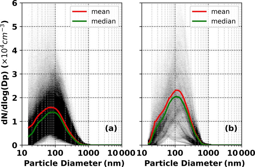
4880                                             J. Qiu et al.: New correction method for a three-wavelength nephelometer

nusoidal function with the nephelometer’s actual scattering
angle sensitivity function to derive the scattering coefficient
under nephelometer light source conditions. The scattering
coefficient under the condition of ideal Lambertian light is
also obtained by the Mie model, which allows calculation of
the CF. However, this method additionally needs the parti-
cle number size distribution (PNSD), particle shape, and re-
fractive index (Quirantes et al., 2008). It is not convenient
to obtain simultaneous PNSD data because the measurement
instrument is expensive and not easy to maintain.
   An alternative popular correction mechanism is to con-
strain the CF simply by the wavelength dependence of scat-
tering (scattering Ångström exponent, SAE). Considering
that the SAE and CF both rely on particle size, Anderson
and Ogren (1998) established a linear relationship between        Figure 1. The number size distribution of the measured aerosol
them for each TSI nephelometer’s wavelength. This inge-           in (a) field observations (1)–(7) and (b) field observation (8).
nious method is convenient because the scattering proper-
ties at different wavelengths, or SAEs, can be directly mea-
sured by the nephelometer itself. However, Bond et al. (2009)
found that the SAE is also affected by the particle refractive
index, while the CF is scarcely impacted by it. This differ-
ence renders the regression method less accurate. Further-
more, the absorption properties of sampled particles can alter
the wavelength dependence of scattering, contributing to er-
rors in this correction method for absorbing aerosols (Bond et
al., 2009). Therefore, it is not an accurate correction method
to establish a simple linear relationship between a single pa-
rameter SAE and CF.
   In this study, the measurement limitations of angle trunca-
tion and the nonideal Lambertian light source are both con-
sidered. In light of the disadvantages of the methods men-
tioned above, we propose a new correction method for the
scattering coefficient measurements of a three-wavelength
nephelometer with the use of a machine learning model and
taking an Aurora 3000 correction as an example. A descrip-
tion of the data and methodology under dry and other relative
humidity conditions is given in Sect. 2. The verifications of
the linear regression method and our new method are pre-          Figure 2. The SSA of field observations (1)–(8).
sented in Sect. 3. Finally, the conclusions are presented in
Sect. 4.

                                                                  aerosols in the North China Plain. Measurements in Bei-
2     Data and method                                             jing were conducted at Peking University (downtown Bei-
                                                                  jing), which is surrounded by two heavy traffic roads and
2.1    Site description                                           hence it can well represent the typical case of urban pol-
                                                                  lution. The number size distribution measurements of the
Eight field observations (Table 1) were conducted at              eight campaigns are obtained by a scanning mobility parti-
different time periods in China, including two obser-             cle size (SMPS) or a twin differential mobility particle sizer
vations in Wuqing (39◦ 380 N, 117◦ 040 E), two in Xi-             (TDMPS) in conjunction with an aerodynamic particle sizer
anghe (39◦ 760 N, 117◦ 010 E), and one observation in each        (APS), and the results cover a wide range of 10–1000 nm
of Wangdu (38◦ 400 N, 115◦ 080 E), Zhangqiu (36◦ 710 N,           (Fig. 1). A 7-wavelength Aethalometer (Model AE33) and
117◦ 540 E), Beijing (39◦ 590 N, 116◦ 180 E), and Gucheng         a Multi-Angle Absorption Photometer (MAAP) are utilized
(38◦ 90 N, 115◦ 440 E). Five sites (Wuqing, Xianghe, Wangdu,      to measure black carbon mass concentration to derive the ab-
Zhangqiu, and Gucheng) are located in suburban areas,             sorption coefficient. The single scattering albedo (SSA) of all
representing the characteristics of regional anthropogenic        field observations varies between 0.235 and 0.997 (Fig. 2).

Atmos. Meas. Tech., 14, 4879–4891, 2021                                             https://doi.org/10.5194/amt-14-4879-2021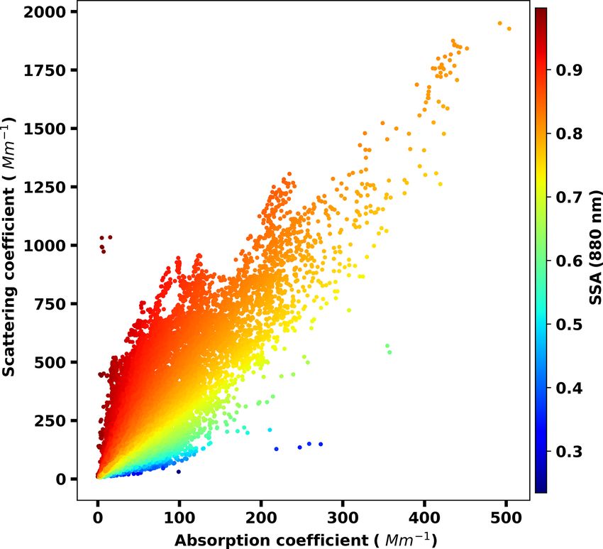
J. Qiu et al.: New correction method for a three-wavelength nephelometer                                                                      4881

Table 1. Summary of the eight field observations used in this paper.

      Site       (1) Wuqing         (2) Wuqing          (3) Xianghe   (4) Xianghe    (5) Wangdu     (6) Zhangqiu   (7) Beijing     (8) Gucheng
      Date       7 March to         12 July to          22 July to    9 July to      4 June to      23 July to     25 March to     15 October to
                 4 April            14 August           30 August     8 August       14 July        24 August      9 April         25 November
      Year       2009               2009                2012          2013           2014           2017           2017            2016
      PNSD       TDMPS +            TDMPS +             SMPS +        TDMPS +        TDMPS +        SMPS +         SMPS +          SMPS +
                 APS                APS                 APS           APS            APS            APS            APS             APS
      BC         MAAP               MAAP                MAAP          MAAP           MAAP           AE33           AE33            AE33
      f (RH)     /                  /                   /             /              TSI 3563       Aurora 3000    Aurora 3000     Aurora 3000

  /: no f (RH) data obtained from that field observation.

2.2     Method                                                                      comes smaller. Therefore, the HBF can to some extent stand
                                                                                    for aerosol size and this paper aims to determine whether the
This paper proposes a simple and precise method of deriv-                           HBF can be used as one parameter to predict the CF or not.
ing the CF. Inspired by establishing a linear relationship be-                      Considering that both the SAE and CF relate to particle size,
tween the SAE and CF (Anderson and Ogren, 1998; Müller                              this paper uses the datasets of field observations (1)–(7) to
et al., 2011), this paper first elucidates more parameters that                     explore the relationship between the CF and the calculated
exert impacts on the CF and can be directly obtained by                             SAE and HBF at different wavelengths (Fig. 3).
nephelometer measurements. Considering the complex rela-                               Following the method of Anderson and Ogren (1998) and
tionships among parameters and the requirements of the or-                          Müller et al. (2011), we established a linear regression equa-
dinary regression method (e.g., independent variables), it is                       tion between the CF and SAE (black dashed lines). It is found
not an appropriate means to use regression analysis to de-                          that the change in the CF could be constrained by the change
rive the relationship between the CF and some variables at                          of the SAE to a certain extent, but the data points are dis-
each wavelength. Therefore, a random forest (RF) machine                            persed from the regression equation. The larger the HBF, the
learning model from the scikit-learn machine learning library                       greater the slope of the CF changes with the SAE. Therefore,
(Pedregosa et al., 2011), an effective method that can be used                      besides the SAE, the HBF can be utilized to provide extra
for classification and nonlinear regression (Breiman, 2001),                        information on particle size and thus predict the CF.
is adopted. The RF model has several advantages (Zhao et                               Before establishing the relationship between the CF and
al., 2018). First, it involves fewer assumptions of dependency                      the calculated SAE and HBF, it is necessary to obtain the size
between observations and results than traditional regression                        range for which particles contribute significantly to the varia-
models. Second, there is no need for a strict relationship                          tions of the SAE and HBF. This paper makes the assumption
among variables before implementing the model simulation.                           that there are three independent types of particle composi-
Third, this model requires much fewer computing resources                           tion: scattering particles, absorbing particles, and core–shell
than deep learning. Finally, it has a lower over-fitting risk.                      mixed particles with a core radius of 35 nm. The refractive
Based on this machine learning model, our new method splits                         index is 1.80 − 0.54i (Ma et al., 2012) for the absorbing ma-
the above datasets into seven training datasets and one test                        terials and 1.53 − 10−7 i (Wex et al., 2002) for the scattering
dataset and then uses the Mie model and the training datasets                       materials. Based on this assumption and all measured size
to calculate the CF. The training dataset CFs, combined with                        distributions mentioned above, the variation of the SAE at the
parameters that impact the CF and can be directly obtained                          three wavelength combinations (450 + 525, 450 + 635, and
from nephelometer, are used to train the machine learning                           525 + 635 nm) and the HBF at the three wavelengths (450,
model. The derived RF models are verified by the test dataset.                      525, and 635 nm) in the particle size range (100 nm–10 µm)
If the verification results are credible, the RF models can be                      is calculated by the Mie model under the Aurora 3000 light
directly used in field measurements to predict the in situ CF                       source conditions (the light angle is limited from 10 to 171◦ ;
and finally obtain the corrected scattering coefficient.                            for details on the angular sensitivity function, please refer
                                                                                    to Müller et al., 2011). Additionally, to distinguish the par-
2.2.1        Correction under dry conditions                                        ticle size range where the change of the SAE and HBF can
                                                                                    be obviously manifested in the overall optical properties of
An important feature of Mie scattering is that the larger the                       aerosols, this paper also calculates the ratio of size-resolved
particle, the more forward scattering, meaning that the ra-                         scattering and hemispheric backscattering to total scattering
tio of the backscattering coefficient to total scattering coeffi-                   for three types of assumed aerosols.
cient, or the hemispheric backscattering fraction (HBF), be-

https://doi.org/10.5194/amt-14-4879-2021                                                              Atmos. Meas. Tech., 14, 4879–4891, 2021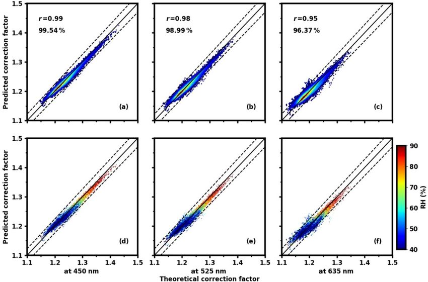
4882                                                J. Qiu et al.: New correction method for a three-wavelength nephelometer

Figure 3. Scattering correction factors versus the scattering Ångström exponent. Panels (a, b, c) represent the results at the wavelengths
of 450, 525, and 635 nm, respectively. The black dashed line is a statistical linear relationship and the color of the points represents the
hemispheric backscattering fraction (HBF).

   As shown in Fig. 4, for all three types of aerosols, scatter-        BC (Mext-BC ) to that of the total BC (MBC ):
ing is mainly concentrated in the size range of 100–1000 nm;
particles larger than 1000 nm contribute little to the total scat-      Rext = Mext-BC MBC .                                            (1)
tering and hence there is no followup discussion of the SAE
                                                                        Ma et al. (2012) pointed out that the HBF is sensitive to Rext .
change of these large particles. When particles are smaller
                                                                        Therefore, on the basis of the Mie model, we use PNSD,
than 1000 nm, the overall trend is that the SAE decreases
                                                                        MBC , and the assumed Rext value to calculate the HBF. Next,
with increasing particle size and that the SAE calculated at
                                                                        the calculation of the HBF is compared with the observation
different wavelengths is obviously different. Especially when
                                                                        results of nephelometers. If their difference is minimal, the
the particle is greater than 300 nm, the SAE variation with
                                                                        assumed Rext value is considered true. Deriving mass con-
particle diameter is large, while particles in the size range of
                                                                        centration of BC and PNSD data, assuming that the true Rext
100–300 nm contribute little to SAE variations. Therefore,
                                                                        is consistent at each size and there is no difference in the
the SAE variability is mostly sensitive to the concentration
                                                                        radius of BC core among core–shell mixed particles of the
of particles in the 300–1000 nm size range.
                                                                        same size, we can calculate the number size distribution of
   From Fig. 5, for environmental aerosol particles the
                                                                        core–shell mixed BC and externally mixed BC. Furthermore,
backscattering of particles in the 100–1000 nm range also
                                                                        the refractive index can also be obtained, making it possible
contributes a lot to the total scattering. The HBF characteris-
                                                                        to derive more precise information of scattering, backscatter-
tics of particles greater than 1000 nm is not discussed further.
                                                                        ing, and then the SAE and HBF. Details about this method of
For particles with a size less than 300 nm, all three types of
                                                                        retrieving PNSD and refractive indices can be found in Ma et
aerosol particles show a noticeable HBF variation with the
                                                                        al. (2012).
change of particle size. However, particles larger than 300 nm
                                                                           In summary, our nephelometer correction method under
contribute little to HBF variations. In other words, HBF vari-
                                                                        dry conditions encompasses the following procedure (Fig. 6):
ability is mostly sensitive to the concentration of particles in
the 100–300 nm size range.                                                1. Obtain information on particle number size distribution
   Based on the above analysis, it is known that the SAE                     (PNSD), black carbon (BC), and mixing state (Rext ) of
and HBF can represent different size information of aerosol                  field observations (1)–(7).
particles (300–1000 nm for the SAE and 100–300 nm for
the HBF), and they are used together to derive the particle               2. Calculate the scattering and backscattering using the
size information in the range of 100–1000 nm. Therefore, the                 Mie model under the nephelometer light source condi-
SAE and HBF are two parameters that can be used for the                      tions at the wavelengths of 450, 525, and 635 nm.
machine learning process.                                                 3. Calculate the hemispheric backscattering fractions
   In order to calculate accurate SAEs and HBFs, scattering                  (HBFs) at the three wavelengths.
and backscattering information should be accurate. Consid-
ering that it is also affected by the mass concentration of BC            4. Calculate the scattering Ångström exponent (SAEs) of
and aerosol mixing states, not only PNSD but also black car-                 the three wavelength combinations (450 + 525, 450 +
bon (BC) data are needed to run the Mie model. According to                  635, and 525 + 635 nm).
Ma et al. (2012), when calculating the amount of externally
mixed BC and core–shell mixed BC, Rext is used to represent               5. Calculate the scattering and backscattering using the
the ratio of the mass concentration of the externally mixed                  Mie model under the ideal light source conditions at the
                                                                             wavelengths of 450, 525, and 635 nm.

Atmos. Meas. Tech., 14, 4879–4891, 2021                                                    https://doi.org/10.5194/amt-14-4879-2021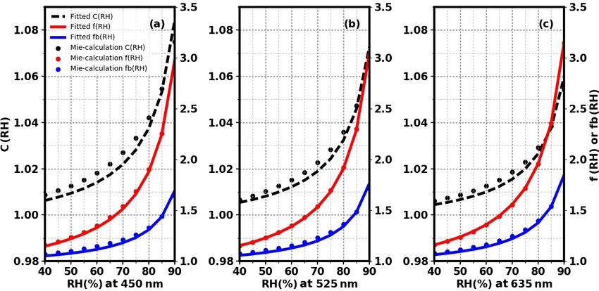
J. Qiu et al.: New correction method for a three-wavelength nephelometer                                                                      4883

Figure 4. The SAE change of scattering particles (a), absorbing particles (b), and core–shell mixing particles of core radius 35 nm (c) with the
change in particle diameter (solid line). The dashed lines represent the ratio of scattering at a certain diameter relative to the total scattering.

  6. Based on the results of the second and fifth steps, calcu-             because, with the increment of relative humidity, the non-
     late the theoretical CF at the three wavelengths.                      absorbing component in the aerosol particle can take up wa-
                                                                            ter due to its hygroscopic growth. Accordingly, the water
  7. Use six parameters, including three HBFs and three                     content and particle size may change, resulting in a certain
     SAEs, and the theoretical CF of each wavelength to                     change in the CF for the same group of aerosol particles.
     train the machine learning model, which derives the RF                 Therefore, besides the SAE and HBF, more parameters re-
     predictor.                                                             lated to hygroscopicity should be considered when deriving
  8. Verify the predictive validity of the trained model with               the CF under elevated relative humidity conditions.
     the dataset of Gucheng.                                                   The hygroscopicity or aerosol hygroscopic growth could
                                                                            be indicated by the scattering hygroscopic growth curve
                                                                            f (RH) and the backscattering hygroscopic growth curve
2.2.2   Correction under different RH conditions                            fb (RH). At low relative humidity, the growth due to an
                                                                            aerosol taking up water is weak and thus the change of
Under elevated relative humidity conditions, a correction                   f (RH) and fb (RH) is small; as relative humidity goes up,
method taking the hygroscopicity into account is needed

https://doi.org/10.5194/amt-14-4879-2021                                                         Atmos. Meas. Tech., 14, 4879–4891, 2021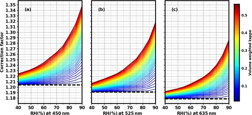
4884                                                 J. Qiu et al.: New correction method for a three-wavelength nephelometer

Figure 5. The HBF change of scattering particles (a), absorbing particles (b), and core–shell mixing particles of core radius 35 nm (c) with
the change in particle diameter (solid line). The dashed lines represent the ratio of hemispheric backscattering at a certain diameter relative
to the total scattering.

the aerosol hygroscopic growth is obvious. Correspondingly,               field observations (Liu et al., 2014), this paper takes their av-
the change of f (RH) and fb (RH) is large. Referring to re-               erage size distribution (the total volume-weighted κ is 0.281)
search by Kuang et al. (2017) and Brock et al. (2016), the                as the basis. Next, in order to obtain a sequence of size dis-
following formulas are used to describe f (RH) and fb (RH):               tributions of κ, the basis κ is multiplied by values rang-
                                                                          ing from 0.05 to 2 with a 0.01 interval. According to the
                     RH                                                   PNSD of outfield observations (1)–(7) and these assumed
f (RH) = 1 + κsca          ,                                     (2)
                  100 − RH                                                size distributions of κ, the theoretical Mie-calculation values
                       RH                                                 are presented as scatter points in Fig. 7. On the basis of the
fb (RH) = 1 + κbsca          ,                                   (3)
                    100 − RH                                              above formulas, the lines represent fitted curves under neph-
where κsca and κbsca are fitting parameters representing the              elometer light source conditions. As can be seen for the three
hygroscopic growth rate in aerosol scattering and backscat-               wavelengths, Eqs. (2) and (3) basically describe the trend of
tering.                                                                   f (RH) and fb (RH) values. In other words, aerosol scatter-
   When it comes to the aerosol overall hygroscopicity, ac-               ing and hemispheric backscattering hygroscopic growth can
cording to 24 size distributions of κ obtained from Hachi                 be represented by parameters of κsca and κbsca . As a result,

Atmos. Meas. Tech., 14, 4879–4891, 2021                                                      https://doi.org/10.5194/amt-14-4879-2021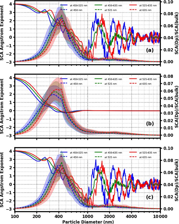
J. Qiu et al.: New correction method for a three-wavelength nephelometer 4885
absolute temperature, Mwater is the molar mass of water, R is
the universal gas constant, and ρw is the density of water.
With the PNSD information, refractive index of the dry
aerosol, mixing state, size distribution of κ, and water refrac-
tive index of 1.33 − 10−7 i (Seinfeld and Pandis, 2006), on
the basis of κ-Köhler theory (Eq. 4), this paper can calculate
the aerosol optical parameters at different RH, which derives
f (RH) and fb (RH). Next, Eqs. (2) and (3) are used to fit the
curve of f (RH) and fb (RH) at each wavelength, thus deriv-
ing the fitting parameters κsca and κbsca , which can imply the
size-resolved hygroscopicity. Combined with relative humid-
ity, the estimated change in the CF with the relative humidity
involves up to 13 physical quantities.
To summarize, our nephelometer correction method under
different relative humidity conditions encompasses the fol-
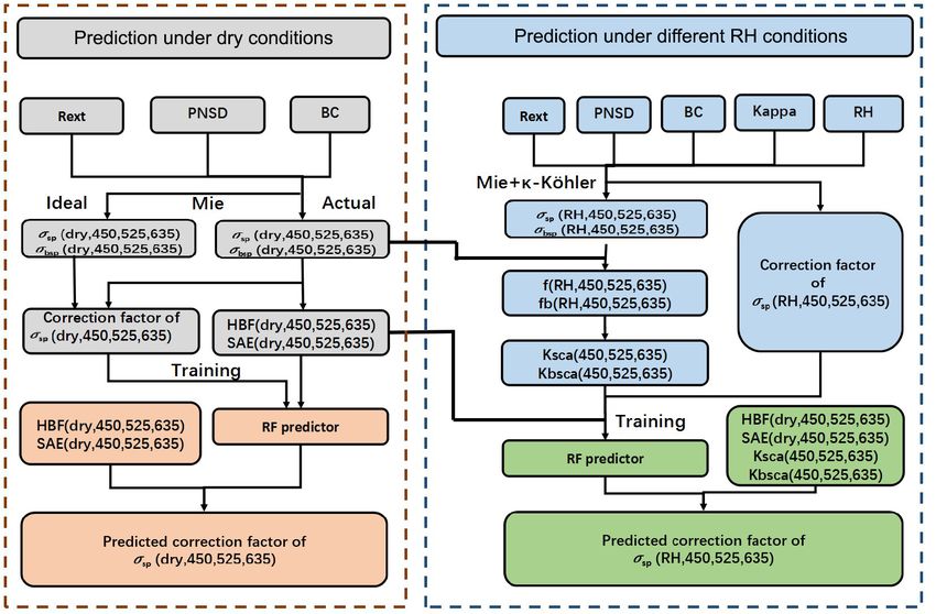
lowing procedure (Fig. 8):
1. Obtain information on particle number size distribution
(PNSD), black carbon (BC), mixing state (Rext ), aerosol
hygroscopicity parameter (κ), and relative humidity RH
of field observations (1)–(7).
2. Calculate the scattering and backscattering using the
Mie model under nephelometer light source conditions
at the wavelengths of 450, 525, and 635 nm in the dry
state.
3. Calculate the hemispheric backscattering fractions
(HBFs) at the three wavelengths under dry conditions.
Figure 6. Flow chart for estimating the CF under dry conditions by
machine learning. 4. Calculate the scattering Ångström exponent (SAEs) of
the three wavelength combinations (450 + 525, 450 +
635, and 525 + 635 nm) under dry conditions.
we wonder whether or not the hygroscopic growth of the CF
(C(RH)) could be fitted similarly as the above formulas with 5. Under different relative humidity conditions and as-
parameter κc . The black scatter points in the figure do not sumptions of aerosol hygroscopicity, according to the
lie close to the black dashed lines and, accordingly, the fit κ-Köhler theory, aerosol scattering and hemispheric
formula cannot accurately describe C(RH). backscattering after the hygroscopic growth are calcu-
Therefore, this paper attempts to derive the CF under dif- lated on the basis of the nephelometer light source at
ferent RH conditions in a similar machine learning way as three wavelengths.
described for the dry state. First of all, we need to find pa-
rameters impacting the CF under different RH conditions. 6. Calculate f (RH) and fb (RH) curves of the three
Aerosol size accounts for the CF, as discussed in Sect. 2.2.1, wavelengths based on the scattering and hemispheric
and thereby the SAE and HBF in the dry state at three wave- backscattering under dry and different relative humid-
lengths are needed. In addition, hygroscopicity matters to ity conditions.
a large extent. κ-Köhler theory (Petters and Kreidenweis,
7. Calculate the fitting parameters of κsca and κbsca from
2008) is thus applied, which uses hygroscopicity parameter κ
f (RH) and fb (RH).
to describe the hygroscopic growth of aerosol particles under
different relative humidity conditions: 8. Calculate the scattering and hemispheric backscattering
after the hygroscopic growth under ideal light source
D 3 − Dd3
4σs/a · Mwater
S= · exp , (4) conditions at three wavelengths.
D 3 − Dd3 (1 − κ) R · T · D · g · ρw
9. Based on the results of the fifth and eighth steps, calcu-
where S is saturation ratio, D is the diameter of the aerosol late the theoretical CF at the three wavelengths.
particle after hygroscopic growth, Dd is the diameter of the
aerosol particle in the dry state, σs/a is the surface tension 10. Use 13 parameters, including three HBFs and three
at the interface between the solution and air, T represents SAEs, relative humidity RH, three κsca and three κbsca
https://doi.org/10.5194/amt-14-4879-2021 Atmos. Meas. Tech., 14, 4879–4891, 2021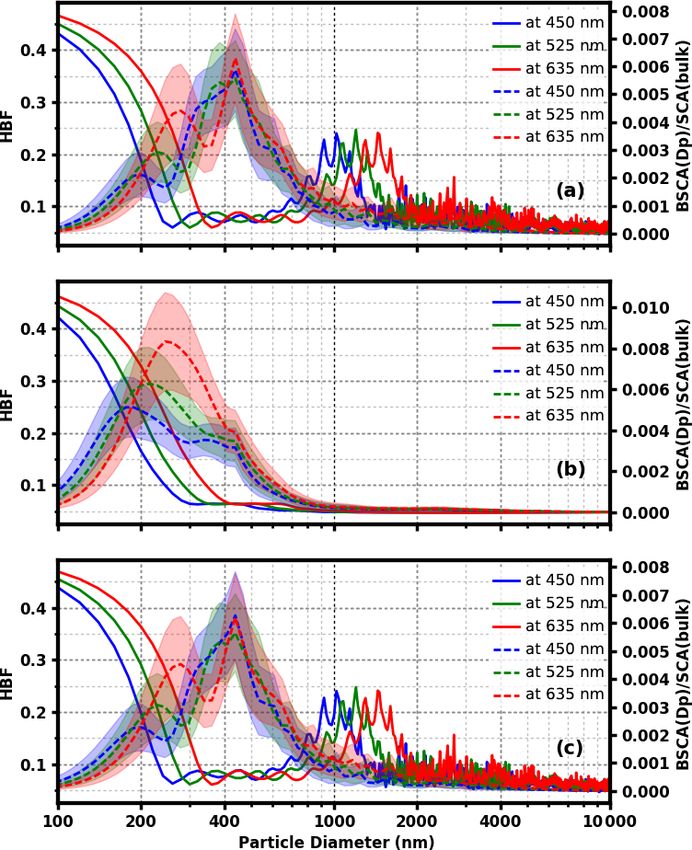
4886                                                   J. Qiu et al.: New correction method for a three-wavelength nephelometer

Figure 7. The comparison between κ fitted and theoretical Mie-calculation f (RH), fb (RH), and C(RH) at the wavelengths of 450 nm (a),
525 nm (b), and 635 nm (c) under nephelometer light source conditions. The scatter points represent each theoretical Mie-calculation value.
The red solid line is the f (RH) fitted curve and the blue solid line is the fb (RH) fitted curve, both corresponding to the right ordinate value.
The black dashed line is the C(RH) fitted curve, which corresponds to the left ordinate value.

Figure 8. Flow chart for estimating the CF under different relative humidity conditions by machine learning.

Atmos. Meas. Tech., 14, 4879–4891, 2021                                                        https://doi.org/10.5194/amt-14-4879-2021
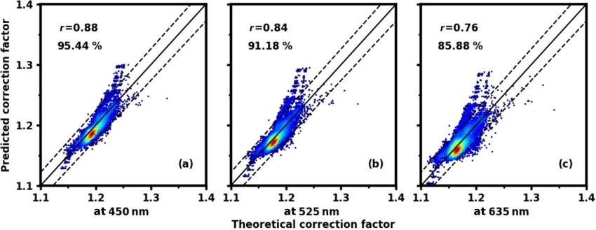
J. Qiu et al.: New correction method for a three-wavelength nephelometer                                                   4887

       at this RH, and the theoretical CF of each wavelength to   the 2 % error range and most of them are basically concen-
       train the machine learning model, which derives the RF     trated near the 1 : 1 line. For 635 nm, the result is slightly
       predictor.                                                 worse, with the correlation coefficient at 0.76 and 85.88 % of
                                                                  the points within the 2 % error range. In general, compared
11. Verify the predictive validity of the trained model with      with the traditional correction method, our method does not
    the dataset of Gucheng.                                       need to consider whether or not the aerosol has strong or
                                                                  wavelength-dependent absorption, which improves the accu-
                                                                  racy of the CF estimation in the dry state; in addition, the
3     Results and discussion                                      input parameters can be obtained by the nephelometer’s ob-
                                                                  servation.
In order to verify the methods introduced above on the ba-
sis of Gucheng data and the derived RF predictor, we have         3.3    Under different RH conditions
predicted the CF and compared it with the theoretical Mie-
calculated CF. First of all, for comparison, Gucheng data are     This paper uses each PNSD of the field observations (1)–
used to verify the simple linear parameterization shown in        (7) and averages them to plot Fig. 12, which represents the
Anderson and Ogren (1998) and Müller et al. (2011).               variation characteristics of the CF with the change of relative
                                                                  humidity and aerosol population hygroscopicity at the three
3.1    Verification of linear regression method                   wavelengths of 450, 525, and 635 nm, respectively.
                                                                     Under all of the different relative humidity conditions, the
The PNSD and BC data of Gucheng are used to establish             CF at 450 nm is the largest, with that of 525 nm coming sec-
linear fit relationships between the CF and the corresponding     ond, and that of 635 nm being the smallest (Fig. 12). All CFs
SAE at three different wavelengths (450, 525, and 635 nm),        at the three wavelengths increase with the increment of rela-
which are, respectively, represented as:                          tive humidity. Furthermore, if the relative humidity remains
                                                                  constant, the CF also increases as aerosol hygroscopicity in-
CF = 1.264 − 0.058SAE,                                      (5)   creases. This is reasonable since the environment relative hu-
CF = 1.260 − 0.059SAE,                                      (6)   midity and the hygroscopicity of aerosols have positive im-
                                                                  pacts on particle sizes and thus the CF.
CF = 1.247 − 0.054SAE.                                      (7)
                                                                     Our correction method under different RH conditions
As shown in Fig. 9, the CF ranges between 1.1 and 1.35.           takes the humidity and hygroscopicity into account. As de-
There is a relatively large gap between the predicted results     picted in Fig. 13, the new method predicts the CF very well
derived from linear relationships and the theoretical simula-     at all the three wavelengths, and nearly all scatter points at
tion result, especially at the wavelengths of 525 and 635 nm.     the three wavelengths are centered near the 1 : 1 line. For the
   When aerosols take up water due to hygroscopic growth          450 nm wavelength, the correlation coefficient between the
with Gucheng data, this paper establishes different linear sta-   prediction value and the theoretical Mie calculation reaches
tistical relationships under different relative humidity condi-   0.99, with 99.54 % of the points falling within the error range
tions in order to estimate the CF. The data points gradually      of 2 %. For the 525 nm wavelength, the correlation coeffi-
become dispersed from the 1 : 1 line as the relative humidity     cient is 0.98, with 98.99 % of the points falling within the
increases (Fig. 10). The reason is that under the condition of    error range of 2 % and for the 635 nm wavelength, the corre-
high humidity, the hygroscopic growth and thus particle size      lation coefficient is 0.95, with 96.37 % of the points in error
can vary greatly due to differences of aerosol hygroscopic-       by less than 2 %. From Fig. 13d–f, the new method’s esti-
ity. Moreover, refractive indices also show large differences     mation of the CF is basically consistent in accuracy at each
owing to the change of water content.                             relative humidity. Another advantage of our new method is
   Therefore, the ordinary linear regression method of estab-     that all these input parameters can be obtained by the neph-
lishing a relationship between the CF and a single parameter      elometer’s observation, achieving the goal of self-correction.
SAE (Anderson and Ogren, 1998; Müller et al., 2011) can-
not be applied to most cases, especially under the condition
of high relative humidity.                                        4     Conclusions

3.2    Under dry conditions                                       The aerosol scattering coefficient is an essential parameter
                                                                  for estimating aerosol direct radiative forcing, which can be
When it comes to the results of our new method, as shown          measured by nephelometers. However, nephelometers have
in Fig. 11 for 450 and 525 nm, the prediction performance is      the problems of a nonideal Lambertian light source and angle
relatively good, and the correlation coefficient between pre-     truncation and hence the observed scattering coefficient data
diction value and the theoretical Mie calculation is 0.88 and     need to be corrected. The scattering correction factor (CF) is
0.84, respectively. More than 90 % of the points fall within      thus proposed and it depends on the aerosol size and chem-

https://doi.org/10.5194/amt-14-4879-2021                                              Atmos. Meas. Tech., 14, 4879–4891, 2021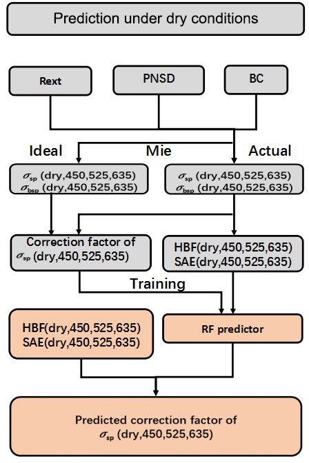
4888                                                  J. Qiu et al.: New correction method for a three-wavelength nephelometer

Figure 9. The comparison of theoretical correction factor and predicted correction factor calculated by the Ångström index at different
wavelengths; panels (a, b, c) are the comparison results for 450, 525, and 635 nm, respectively. The black solid line represents that the
theoretical correction factor equals the predicted one. The color of the data points represents the data density; the warmer the hue, the denser
the data points.

Figure 10. The comparison of theoretical correction factor and predicted correction factor calculated by the Ångström index at different
wavelengths; panels (a, b, c) are the comparison results for 450, 525, and 635 nm, respectively. The black solid line represents that the
theoretical correction factor equals the predicted one. The color of the data points represents different relative humidity conditions.

Figure 11. Under dry conditions, the comparison of the correction factors calculated by our method and the theoretical Mie-calculation values
at the wavelengths of 450 nm (a), 525 nm (b), and 635 nm (c), respectively, with a black solid 1 : 1 line and two dashed lines representing
a deviation of 2 %. The color of the data points represents data density; the warmer the hue, the denser the data point. r is the correlation
coefficient, and the percentage indicates the percentile of points falling within the error range of 2 %.

Atmos. Meas. Tech., 14, 4879–4891, 2021                                                      https://doi.org/10.5194/amt-14-4879-2021
J. Qiu et al.: New correction method for a three-wavelength nephelometer                                                                     4889

Figure 12. The theoretical calculation of the scattering correction factors (CFs) versus relative humidity (RH) and hygroscopicity κ at the
wavelengths of 450 nm (a), 525 nm (b), and 635 nm (c). The dashed line represents a scattering correction factor in the dry state and the
color represents the overall hygroscopicity of aerosols (κ). The color bar is derived from multiplying the total volume-weighted κ of 0.281
by values ranging from 0.05 to 2 with a 0.01 interval.

Figure 13. At different relative humidity conditions, the comparison of the correction factors calculated by our method and the theoretical
Mie-calculation values at the wavelengths of 450 nm (a), 525 nm (b), and 635 nm (c), respectively, with a black solid 1 : 1 line and two dashed
lines representing a deviation of 2 %. The color of the data points represents data density; the warmer the hue, the denser the data point. r is
the correlation coefficient, and the percentage indicates the percentile of points falling within the error range of 2 %. The data in (d, e, f) are
the same as those in (a, b, c), but the color here stands for different relative humidity conditions rather than density.

ical composition. The most direct calibration method is to                  fore, our paper has proposed a new method of nephelometer
combine the particle number size distribution, black carbon                 self-correction.
data, and Mie scattering model to correct the nephelometer.                    Under dry conditions and after the analysis, the SAE and
However, this method requires auxiliary measurement data.                   HBF can represent different ranges of aerosol particle size
After proposing this method, the scattering Ångström expo-                  information (300–1000 nm for the SAE and 100–300 nm for
nent (SAE) measured by nephelometer itself is utilized to es-               the HBF). With the use of the existing observation results of
tablish a linear relationship with the CF. After verification, it           PNSD, black carbon, and Rext to obtain the SAE and HBF,
is found that the method lacks precision and accuracy. There-               this paper applies the random forest (RF) machine learning

https://doi.org/10.5194/amt-14-4879-2021                                                        Atmos. Meas. Tech., 14, 4879–4891, 2021
4890                                               J. Qiu et al.: New correction method for a three-wavelength nephelometer

model to establish the relationship between the CF and the          this method, hopefully establishing a database of RF models
calculated SAE and HBF, and ultimately derives the trained          in the future.
RF model. With the dataset of Gucheng, the verification re-
sults show that this method is relatively accurate. The com-
monly used integrating nephelometer can derive in situ scat-        Code and data availability. The     data    and       codes used
tering and backscattering coefficients at three wavelengths to      in this study are available by request to the author
calculate three SAEs and three HBFs. Therefore, with the            (email: zcs@pku.edu.cn). They can also be obtained from
use of the derived RF model and the nephelometer calcula-           https://pan.baidu.com/s/1AhAa6yz5VwDi0tTflH4m9g (the pass-
                                                                    word is scp0; last access: 18 May 2021, Qiu et al., 2021).
tion of the SAE and HBF, the CF could be predicted by the
nephelometer itself.
   Under other relative humidity conditions, the humidified
                                                                    Author contributions. JQ, WT, GZ, YY, and CZ discussed the re-
nephelometer system is utilized. In addition to the dry aerosol     sults; WT offered his help with the coding; and JQ wrote the
particle size information, we should also consider the change       manuscript.
in water content and particle size brought by the growth of
aerosol taking up water. This paper finds that the CF in-
creases with the increment of relative humidity and aerosol         Competing interests. The authors declare that they have no conflict
hygroscopicity. Therefore, on the basis of κ-Köhler theory,         of interest.
the existing observation results of PNSD, black carbon, Rext ,
aerosol hygroscopicity parameter κ, and relative humidity
are used to run the Mie model, obtaining the theoretical CF         Disclaimer. Publisher’s note: Copernicus Publications remains
and 13 quantities relating to the CF change under differ-           neutral with regard to jurisdictional claims in published maps and
ent RH conditions. Similarly, the machine learning model            institutional affiliations.
is trained to obtain the relationship between the CF and the
13 quantities. With the dataset of Gucheng, the verification
results show that the accuracy of the CF obtained by this           Acknowledgements. We acknowledge the support of the National
method is very high. The humidified nephelometer system             Natural Science Foundation of China.
can observe scattering and hemispheric backscattering coef-
ficients at three wavelengths under both dry and elevated RH
conditions, obtaining the corresponding f (RH) and fb (RH)          Financial support. This research has been supported by the Na-
                                                                    tional Natural Science Foundation of China (grant no. 41590872).
under the nephelometer light source conditions. As a result,
all 13 quantities, including six physical quantities of SAEs
and HBFs representing dry aerosol size at each wavelength,
                                                                    Review statement. This paper was edited by Paolo Laj and re-
six fitting parameters κsca and κbsca representing particle size-
                                                                    viewed by three anonymous referees.
resolved hygroscopicity at each wavelength, and the rela-
tive humidity, can be directly obtained from nephelometers.
Therefore, with the use of the derived RF model and the
above 13 quantities, the CF could be predicted in situ by the       References
humidified nephelometer system.
                                                                    Anderson, T. L. and Ogren, J. A.: Determining aerosol
   The strengths of our new method are summed up as fol-
                                                                      radiative properties using the TSI 3563 integrat-
lows: under either dry or any other relative humidity condi-          ing nephelometer, Aerosol Sci. Tech., 29, 57–69,
tions, the prediction performance of the CF at three wave-            https://doi.org/10.1080/02786829808965551, 1998.
lengths is excellent. Furthermore, at each relative humidity,       Anderson, T. L., Covert, D. S., Marshall, S. F., Laucks, M. L., Charl-
the accuracy of the CF estimation is almost the same. All             son, R. J., Waggoner, A. P., Ogren, J. A., Caldow, R., Holm, R. L.,
inputs can be obtained through the nephelometer’s observa-            Quant, F. R., Sem, G. J., Wiedensohler, A., Ahlquist, N. A., and
tions, thus achieving self-correction; that is, on the basis of       Bates, T. S.: Performance characteristics of a high-sensitivity,
ensuring the accuracy of correction, there is no need for other       three-wavelength, total scatter/backscatter nephelometer, J. At-
aerosol microphysical observations.                                   mos. Ocean. Tech., 13, 967–986, https://doi.org/10.1175/1520-
   Due to the limitations of Mie theory, our method cannot            0426(1996)0132.0.CO;2, 1996.
                                                                    Bond, T. C., Covert, D. S., and Müller, T.: Truncation and
be applied to analyze datasets that include desert and marine
                                                                      angular-scattering corrections for absorbing aerosol in the
aerosols and hence further studies are needed. In this study,         TSI 3563 nephelometer, Aerosol Sci. Tech., 43, 866–871,
the new method is put forward only based on datasets in the           https://doi.org/10.1080/02786820902998373, 2009.
North China Plain. There might be errors in applying our RF         Breiman, L.: Random forests, Mach. Learn., 45, 5–32,
models to predict the CF all over the world. Therefore, more          https://doi.org/10.1023/A:1010933404324, 2001.
field observation datasets are needed to verify and perfect         Brock, C. A., Wagner, N. L., Anderson, B. E., Attwood, A. R.,
                                                                      Beyersdorf, A., Campuzano-Jost, P., Carlton, A. G., Day, D. A.,

Atmos. Meas. Tech., 14, 4879–4891, 2021                                                https://doi.org/10.5194/amt-14-4879-2021
J. Qiu et al.: New correction method for a three-wavelength nephelometer 4891 Diskin, G. S., Gordon, T. D., Jimenez, J. L., Lack, D. A., Liao, Pedregosa, F., Varoquaux, G., Gramfort, A., Michel, V., Thirion, B., J., Markovic, M. Z., Middlebrook, A. M., Ng, N. L., Perring, Grisel, O., Blondel, M., Louppe, G., Prettenhofer, P., Weiss, R., A. E., Richardson, M. S., Schwarz, J. P., Washenfelder, R. A., Weiss, R. J., Vanderplas, J., Passos, A., Cournapeau, D., Brucher, Welti, A., Xu, L., Ziemba, L. D., and Murphy, D. M.: Aerosol M., Perrot, M., and Duchesnay, E.: Scikit-learn: Machine Learn- optical properties in the southeastern United States in summer ing in Python, J. Mach. Learn. Res., 12, 2825–2830, 2011. – Part 1: Hygroscopic growth, Atmos. Chem. Phys., 16, 4987– Petters, M. D. and Kreidenweis, S. M.: A single parameter repre- 5007, https://doi.org/10.5194/acp-16-4987-2016, 2016. sentation of hygroscopic growth and cloud condensation nucleus IPCC: Climate Change 2013 – The Physical Science Basis: Contri- activity – Part 2: Including solubility, Atmos. Chem. Phys., 8, bution of the Working Group I to the Fifth Assessment Report of 6273–6279, https://doi.org/10.5194/acp-8-6273-2008, 2008. the IPCC, Cambridge University Press, New York, NY, 2013. Qiu, J., Tan, W. S., Zhao, G., Yu, Y. L., and Zhao, C. S.: python3- Kuang, Y., Zhao, C., Tao, J., Bian, Y., Ma, N., and Zhao, AMT, pan.baidu [data set and code], available at: https://pan. G.: A novel method for deriving the aerosol hygroscopic- baidu.com/s/1AhAa6yz5VwDi0tTflH4m9g, last access: 18 May ity parameter based only on measurements from a humidi- 2021. fied nephelometer system, Atmos. Chem. Phys., 17, 6651–6662, Quirantes, A., Olmo, F. J., Lyamani, H., and Alados-Arboledas, https://doi.org/10.5194/acp-17-6651-2017, 2017. L.: Correction factors for a total scatter/backscatter neph- Liu, H. J., Zhao, C. S., Nekat, B., Ma, N., Wiedensohler, A., elometer, J. Quant. Spectrosc. Ra., 109, 1496–1503, van Pinxteren, D., Spindler, G., Müller, K., and Herrmann, https://doi.org/10.1016/j.jqsrt.2007.12.014, 2008. H.: Aerosol hygroscopicity derived from size-segregated Seinfeld, J. H. and Pandis, S. N.: Atmospheric chemistry and chemical composition and its parameterization in the physics: from air pollution to climate change, John Wiley & North China Plain, Atmos. Chem. Phys., 14, 2525–2539, Sons, New York, USA, 701–1118, 2006. https://doi.org/10.5194/acp-14-2525-2014, 2014. Wex, H., Neususs, C., Wendisch, M., Stratmann, F., Koziar, C., Ma, N., Zhao, C. S., Müller, T., Cheng, Y. F., Liu, P. F., Deng, Z. Keil, A., Wiedensohler, A., and Ebert, M.: Particle scatter- Z., Xu, W. Y., Ran, L., Nekat, B., van Pinxteren, D., Gnauk, T., ing, backscattering, and absorption coefficients: An in situ Müller, K., Herrmann, H., Yan, P., Zhou, X. J., and Wiedensohler, closure and sensitivity study, J. Geophys. Res., 107, 8122, A.: A new method to determine the mixing state of light absorb- https://doi.org/10.1029/2000jd000234, 2002. ing carbonaceous using the measured aerosol optical properties Zhao, G., Zhao, C., Kuang, Y., Bian, Y., Tao, J., Shen, C., and and number size distributions, Atmos. Chem. Phys., 12, 2381– Yu, Y.: Calculating the aerosol asymmetry factor based on mea- 2397, https://doi.org/10.5194/acp-12-2381-2012, 2012. surements from the humidified nephelometer system, Atmos. Müller, T., Laborde, M., Kassell, G., and Wiedensohler, A.: Design Chem. Phys., 18, 9049–9060, https://doi.org/10.5194/acp-18- and performance of a three-wavelength LED-based total scatter 9049-2018, 2018. and backscatter integrating nephelometer, Atmos. Meas. Tech., 4, 1291–1303, https://doi.org/10.5194/amt-4-1291-2011, 2011. https://doi.org/10.5194/amt-14-4879-2021 Atmos. Meas. Tech., 14, 4879–4891, 2021
You can also read