On the Treatment of Relative-Pose Measurements for Mobile Robot Localization

Page created by Melanie Warren
 
CONTINUE READING
On the Treatment of Relative-Pose Measurements for Mobile Robot Localization
On the Treatment of Relative-Pose Measurements
                        for Mobile Robot Localization
                                      Anastasios I. Mourikis and Stergios I. Roumeliotis
                 Dept. of Computer Science & Engineering, University of Minnesota, Minneapolis, MN 55455
                                          Email: {mourikis|stergios}@cs.umn.edu

   Abstract— In this paper, we study the problem of localization      exteroceptive measurements are employed to infer robot dis-
using relative-state estimates. It is shown, that when the same       placement is that consecutive relative-state measurements are
exteroceptive sensor measurement is processed for the compu-          stochastically correlated. The correlation is introduced from
tation of two consecutive displacement estimates (both forward
and backward in time) these estimates are correlated, and an          the fact that the measurements recorded at time-step k (e.g., the
analysis of the exact structure of the correlations is performed.     relative positions of landmarks) are used in order to estimate the
This analysis is utilized in the design of data fusion algorithms,    displacement during the time intervals [k − 1, k] and [k, k + 1].
that correctly account for the existing correlations. We examine      As a result, any errors in the measurements at time step k affect
two cases: i) pose propagation based exclusively on inferred          both displacement estimates, thereby rendering them correlated.
displacement measurements, and ii) the fusion of proprioceptive
sensor information with relative-state measurements. For the latter   If the measurements are treated as being uncorrelated (as is
case, an efficient EKF-based estimation algorithm is proposed,        customarily done [9], [1], [3]) information is lost, and the
that extends the approach of [1]. Extensive simulation and            estimates for the robot’s state and covariance are not optimal.
experimental results are presented, that verify the validity of the   This fact has been generally overlooked in the literature, and,
presented method.                                                     to the best of our knowledge, no prior work exists that directly
                                                                      addresses this issue.
                       I. I NTRODUCTION
                                                                         In this paper, we propose a direct approach to the processing
   Accurate localization is a prerequisite for a robot to be able     of correlated displacement measurements, that extends the
to interact with its environment in a meaningful way. The             Stochastic Cloning Kalman Filter (SC-KF) algorithm of [1].
most commonly available sensors for acquiring localization            In particular, in Section III we show how the correlation of
information are proprioceptive sensors, such as wheel encoders,       the measurements can be accounted for, when propagating
gyroscopes, and accelerometers, that provide information about        the covariance of the robot’s pose in time, based only on
the robot’s motion. By integrating proprioceptive measurements        relative-state measurements. Additionally, in Section IV we
over time, it is possible to estimate the total displacement          propose a formulation of the Extended Kalman Filter (EKF)
from a starting point, and this method of localization is             for fusing proprioceptive and relative-state measurements, that
often called Dead Reckoning (DR) [2]. The limitation of               correctly treats correlation between consecutive measurements.
DR is that since no external reference signals are employed           This is achieved by augmenting the state vector to include
for correction, estimation errors accumulate over time, and           the measurement errors for each exteroceptive measurement.
the pose estimates drift from their real values. In order to          The simulation and experimental results from the application
improve the accuracy of localization, most algorithms fuse the        of this method demonstrate that correctly accounting for the
proprioceptive information with data from exteroceptive sensors       correlations results in better state estimates, as well as in
(such as cameras [3], [4], laser range finders [5] sonars [6],        covariance estimates that reflect the true uncertainty in the
etc) that provide measurements of parameters of interest in the       robot’s pose more accurately.
environment.
   When an exteroceptive sensor measures the position of a                                 II. R ELATED W ORK
set of features with respect to the robot at two different time          Once a displacement measurement is derived from an ex-
instants, then it is possible (under necessary observability as-      teroceptive sensor, in most cases it must be combined with
sumptions) to create an inferred measurement of the robot’s dis-      other position estimates derived from onboard proprioceptive
placement. Examples of algorithms that process exteroceptive          sensors. An appealing solution to this problem is to use the
data to infer motion include laser scan matching [5], [7], vision-    previous position estimates for converting the relative-pose
based motion estimation techniques using stereoscopic [3], [4],       measurements to absolute position pseudo-measurements, and
and monocular [8] image sequences, and matching of sonar              treat them as such [10]. However, this approach is correct
returns [6]. The inferred relative-state measurements that are        only when the orientation of the vehicle is precisely known.
produced can either be integrated over time to provide pose           Moreover, to guarantee consistency of the pose estimates,
estimates for the robot’s state at each time instant [4], or fused    the covariance matrix of the pseudo-measurements has to be
with proprioceptive sensory input, in order to benefit from both      artificially inflated [11].
available sources of positioning information [1].                        A difficulty that arises when processing relative-pose mea-
   A characteristic which is common in most cases where               surements is the existence of correlations between consecutive
measurement errors (cf. Section III). A simplistic approach to                     These are, for example, the measurements of the position of
this problem would be to discard correlations, by separating                       landmarks with respect to the robot, or the range measurements
the measurements recorded at each robot pose in two non-                           of a laser range finder. By processing these measurements
overlapping sets; one is used to estimate motion forward in                        (for example, by performing laser scan matching), an estimate,
time, while the second is used to estimate displacement back-                      zk/k+1 , for the change in the robot pose between time-steps k
ward in time. This solution, however, would be far from opti-                      and k + 1 is computed, which is described by a function (either
mal, as it would result in less accurate displacement estimates.                   closed-form or implicit):
An indirect solution is to avoid the introduction of correlations
                                                                                                    zk/k+1    =      ξk/k+1 (zk , zk+1 )           (1)
altogether, by not using the exteroceptive measurements to infer
displacement directly. In this formulation, the robot’s pose and                   Linearization of this last expression enables us to relate the
the position of the environmental features are estimated jointly,                  error in the displacement estimate, zek/k+1 , to the errors in the
thus introducing the well-known Simultaneous Localization and                      exteroceptive measurements:
Mapping (SLAM) problem, which has been extensively studied                                                         k            k+1
in the robotics community (e.g., [12], [13], [14]). If an exact                                 zek/k+1   '       Jk/k+1 zek + Jk/k+1 zek+1        (2)
solution to SLAM was possible, the resulting pose estimates                        Here, we assume that the errors in the exteroceptive mea-
would be optimal, since all the positioning information is                         surements, zek and zek+1 , are zero-mean and independent, an
used, and all the inter-dependencies between the robot and the                     assumption which holds in most practical cases, when proper
feature states are accounted for. However, the major limitation                                                                          k
                                                                                   sensor characterization is performed. In Eq. (2) Jk/k+1      and
of SLAM is that its computational complexity and memory                              k+1
                                                                                   Jk/k+1 are the Jacobians of the function ξk/k+1 (zk , zk+1 ) with
requirements increase quadratically with the number of features
                                                                                   respect to zk and zk+1 , respectively, i.e.,
in the environment. This implies that, if a robot operates over
                                                                                        k                                   k+1
extended periods of time, the amount of resources that need                            Jk/k+1 = ∇zk ξk/k+1         and     Jk/k+1 = ∇zk+1 ξk/k+1
to be allocated for localization tend to become unacceptably
large, if real-time performance is necessary.                                      Once the displacement estimate zk/k+1 between time-steps k
   In this paper, we propose an algorithm for fusing propri-                       and k + 1 has been computed, the pose estimate for the robot
oceptive information with relative-state measurements, which                       at time step k + 1 is evaluated by combining the previous pose
extends the SC-KF algorithm [1], to be applicable to the case                      estimate and the displacement information, by an appropriate,
of correlated relative-state measurements. In our algorithm,                       generally nonlinear function:
the exteroceptive measurements are considered in pairs of                                             bk+1
                                                                                                      X               bk , zk/k+1 )
                                                                                                                  = g(X                            (3)
consecutive measurements, that are first processed in order to
create an inferred relative-state measurement, and then fused                      By linearizing this equation, the pose errors at time step k + 1
with the proprioceptive measurements. The sole objective of the                    can be related to the error in the previous state estimate and
algorithm is the estimation of the robot’s state, and therefore                    that in the displacement measurement:
we do not estimate the states of features in the environment.                                      ek+1
                                                                                                   X          '        ek + Γk zek/k+1
                                                                                                                    Φk X                           (4)
Our motivation for this arises from the fact that in applica-
tions where building a map is not necessary, the overhead                          where Φk and Γk represent the Jacobians of the state prop-
of performing SLAM may not be justified. In cases where                            agation function, g(X  bk , zk/k+1 ), with respect to the previous
real-time performance is required (e.g., autonomous aircraft                       pose, and the relative pose measurement, respectively. During
landing), the proposed algorithm is able to optimally fuse                         localization, it is necessary to provide a measure of the quality
the, potentially correlated, relative-state measurements, with                     of the pose estimates, since the uncertainty in the robot’s pose
the minimum computational overhead. Before presenting this                         should be taken into consideration for motion planning and
algorithm, in the following section we analyze the structure                       navigation. For a Gaussian distribution, a sufficient indicator
of the correlations that exist between consecutive displacement                    of uncertainty is the covariance matrix of the pose errors:
measurements, and demonstrate how these should be treated in                                      ek+1 X
                                                                                                       ek+1
                                                                                                         T
                                                                                      Pk+1    = E{X         }
the propagation of the pose estimates’ uncertainty.
                                                                                              = Φk Pk ΦTk + Γk Rk/k+1 ΓTk
         III. C OVARIANCE P ROPAGATION BASED ON                                                        ek zeT                      ekT }ΦTk (5)
              D ISPLACEMENT M EASUREMENTS                                                     + Φk E{X          }ΓTk + Γk E{e
                                                                                                              k/k+1         zk/k+1 X
   In this section, we consider the case in which the pose                         where Rk/k+1 denotes the covariance matrix of the displace-
estimate of a robot1 , Xbk , is propagated in time using only                      ment estimates. If the measurement noise, zek/k+1 , and state er-
displacement estimates, that are acquired by processing extero-                         ek , are uncorrelated, the last two terms in Eq. (5) are equal
                                                                                   ror, X
ceptive measurements. Let zk and zk+1 denote the vectors of                        to zero matrices, and the covariance propagation expression
exteroceptive measurements at time-steps k and k + 1, respec-                      becomes identical to the well-known covariance propagation
tively, whose covariance matrices are denoted as Rk and Rk+1 .                     expression of the Extended Kalman Filter [15]. Although this
  1 Throughout this paper, the “hat” symbol, b , is used to denote the estimated
                                                                                   is a common assumption in the literature (e.g., [1], [9]), we
value of a quantity, while the “tilde” symbol, e , is used to signify the error
                                                                                   now demonstrate that it does not hold in general, and the last
                                                               e=x−x
between the actual value of a quantity and its estimate, i.e., x         b.        two terms in Eq. (5) are not equal to zero. In particular, by
linearizing the state propagation equation at time-step k, we        the independence of the measurements [15]. To address the
obtain (cf. Eq. (4)):                                                first challenge, we adopt the approach proposed in [1], that
                      ½      ³                          ´T ¾         requires the augmentation of the EKF (error) state vector2
E{e         e T                      e
    zk/k+1 Xk } = E zek/k+1 Φk−1 Xk−1 + Γk−1 zek−1/k                 to include two copies of the robot’s error state (cloning).
                                                                     The first copy represents the pose error at the time instant
           = E{e      ek−1
               zk/k+1 X T
                           }ΦTk−1 + E{e        T
                                      zk/k+1 zek−1/k }ΓTk−1          when the latest exteroceptive measurement was recorded, while
                        T
           = E{e
               zk/k+1 zek−1/k }ΓTk−1                          (6)    the second copy represents the error in the robot’s current
                                                                     state. Consequently, the robot states that are related by each
At this point we note that the error term X    ek−1 depends on       displacement estimate are represented explicitly in the filter
the measurement errors of all exteroceptive measurements up          state.
to, and including, time-step k − 1, while the error term zek/k+1        The second challenge is addressed by further augmenting
depends on the measurement errors at time-steps k and k + 1          the state vector to include the errors of the latest exteroceptive
(cf. Eq. (2)). As a result, the errors X  ek−1 and zek/k+1 are       measurement. Thus, if the most recent exteroceptive measure-
independent, and therefore, by applying the zero-mean assump-        ment was recorded at time-step k, the filter’s state vector at
tion for the error zek/k+1 we obtain E{e  zk/k+1 Xe T } = 0. In      time-step k + i is given by3
                                                   k−1
                                        T                                                        h                      iT
order to evaluate the term E{e zk/k+1 zek−1/k }, which expresses
the correlation between the consecutive displacement estimates,                   X̆k+i|k = X      eT     eT
                                                                                                          X         z
                                                                                                                    e T
                                                                                                                                    (9)
                                                                                                    k|k     k+i|k    k
we employ Eq. (2), and the independence of exteroceptive
measurement errors at different time-steps, to obtain:               By including the measurement error in the state vector of
                                                                     the system, the dependency of the relative-state measure-
                  T               k
       E{e
         zk/k+1 zek−1/k }    =   Jk/k+1   zk zekT }Jk−1/k
                                        E{e         k T
                                                                     ments zk/k+1 on the exteroceptive measurements zk is trans-
                             =    k
                                 Jk/k+1     k T
                                        Rk Jk−1/k             (7)    formed into a dependency on the current state of the filter, and
                                                                     the problem can now be treated in the standard EKF framework.
This result implies that consecutive displacement estimates are      It should be noted, that since the error in the intermediate
not independent. However, the statistical correlation between        measurement is the source of the correlation between the
them is computable in closed form, and can be accounted for          current and previous displacement estimates (cf. Eq. (7)), this
in the propagation of the state covariance matrix. Substituting      is the “minimum length” vector that we need to append to
from Eqs. (6) and (7) into Eq. (5), we obtain the final ex-          the state vector, in order to sufficiently describe the existing
pression for propagating the pose covariance based on inferred       dependencies. In the following sections, we present in detail
displacement measurements:                                           the propagation and update phases of the filter.
    Pk+1    =                                       T
                Φk Pk ΦTk + Γk Rk/k+1 ΓTk + Dk+1 + Dk+1 (8)          A. State propagation
with                                                                   Consider the case where the filter’s state covariance matrix,
             Dk+1 =            k
                      Φk Γk−1 Jk−1/k     k T
                                     Rk Jk/k+1 ΓTk                   immediately after the exteroceptive measurement zk has been
                                                                     processed, is given by:
The experimental results presented in Section V-B demonstrate,                                                       
that by employing this expression for propagating the robot’s                                  Pk|k     Pk|k PXk zk
pose covariance matrix, we are able to compute covariance                        P̆k|k =  Pk|k         Pk|k PXk zk           (10)
                                                                                                T        T
estimates that accurately represent the robot’s uncertainty.                                  PX  k zk
                                                                                                       P Xk zk    R k

    IV. F ILTERING WITH CORRELATED RELATIVE - STATE                  where Pk|k is the covariance of the actual robot pose at time-
                       MEASUREMENTS                                  step k, Rk is the covariance matrix of the error zek , and
                                                                     PXk zk = E{X  ek zeT } is the cross-correlation between the robot’s
                                                                                        k
   In this section, we consider the situation in which relative-
                                                                     state and the measurement error at time-step k (the derivation of
state measurements are fused with proprioceptive sensory in-
                                                                     a closed-form expression for PXk zk is presented in Section IV-
formation to estimate the robot’s pose. Since the propriocep-
                                                                     B). We note that cloning the robot’s state creates two random
tive and exteroceptive measurements are received from two
                                                                     variables that convey the same information, and hence are fully
independent sources of information, fusing them will always
                                                                     correlated [1]. This explains the structure of the covariance
result in superior estimation accuracy, compared to the accuracy
                                                                     matrix in Eq. (10).
attainable when the robot’s pose is propagated based solely on
                                                                        Between two consecutive updates, the proprioceptive mea-
one of the two types of measurements.
                                                                     surements are employed to propagate the filter’s state and its
   Two challenges arise when fusing relative-state and propri-
                                                                     covariance. Let the proprioceptive measurement at time-step
oceptive measurements: firstly, since each displacement mea-
                                                                     k be denoted as vk , and its noise covariance matrix as Qk .
surement relates the robot’s state at two different time instants,
the “standard” formulation of the EKF, in which the filter’s state      2 Since the EKF is employed for estimation, the state vector comprises of the

comprises only the current state of the robot, is not adequate.      errors in the estimated quantities, rather than the estimates. Therefore, cloning
                                                                     has to be applied to both the error states, and the actual estimates.
Secondly, as shown in the preceding section (cf. Eq. (7)), the          3 In the remainder of the paper the subscript `|j denotes the estimated value
consecutive displacement measurements are correlated, and this       of a quantity at time step `, after exteroceptive measurements up to time-step j,
violates one of the basic assumptions of the EKF, that of            and proprioceptive measurements up to time-step ` − 1, have been processed.
The estimate for the robot’s pose is propagated in time by the,     The expected value of zk/k+m is computed based on the
generally non-linear, equation:                                     estimates for the state at times k and k + m, as zbk/k+m =
                                                                    h(Xbk|k , X
                                                                              bk+m|k ), and therefore the innovation is given by:
                     bk+1|k
                     X                 bk|k , vk )
                                  = f (X                    (11)
                                                                    r   =    zk/k+m − zbk/k+m
Linearization of the last expression yields the error propagation                                                 
equation for the (evolving) robot state:                                     h                         i     Xek|k
                                                                        '     Hk    Hk+m       k
                                                                                              Jk/k+m       X
                                                                                                            ek+m|k  + Jk/k+m
                                                                                                                        k+m
                                                                                                                              zek+m
                  ek+1|k
                  X           '        ek|k + Gk vek
                                    Fk X                    (12)
                                                                                                              zek
where Fk and Gk are the Jacobians of f (X    bk+1|k , vk ) with         =                     k+m
                                                                             H̆k+m X̆k+m/k + Jk/k+m zek+m                             (18)
            b
respect to Xk|k and vk , respectively. Since the cloned state,
as well as the estimates for the measurement error zek do           where Hk (Hk+m ) is the Jacobian of h(Xk , Xk+m ) with
                                                                                                k          k+m
not change with the incorporation of a new proprioceptive           respect to Xk (Xk+m ), and Jk/k+m   (Jk/k+m  ) is the Jacobian
measurement, the error propagation equation for the entire state    of zk/k+m = ξk/k+m (zk , zk+m ) with respect to zk (zk+m ).
vector is given by
                X̆k+1|k = F̆k X̆k|k + Ğk vek               (13)       The result of Eq. (18) demonstrates that by incorporating the
                                                                measurement errors, zek , in the state vector, the only component
                  I 0 0                        0                    of the innovation that is not dependent on the state is the
with    F̆k   = 0 Fk 0 and Ğk = Gk                     (14)    measurement noise, zek+m , which is independent of all other
                  0 0 I                        0                    error terms in Eq. (18). Thus, the Kalman filter equations can
thus the covariance matrix of the propagated filter state is:       be applied to update the state. The covariance of the residual
                                                                    is equal to
              P̆k+1|k = F̆k P̆k|k F̆kT + Ğk Qk ĞTk        (15)                                 T      k+m         k+m T
                                                                        S̆   =   H̆k+m P̆k+m|k H̆k+m + Jk/k+m Rk+m Jk/k+m (19)
It is straightforward to show by induction that if m propagation
steps take place between two consecutive relative-state updates     while the Kalman gain is computed as:
the covariance matrix P̆k+m|k is determined as                                            T
                                                                                                     £                           ¤T
                                                                        K̆ = P̆k+m|k H̆k+m    S̆ −1 = KkT          T
                                                                                                                  Kk+m    KzTk        (20)
                                 T                           
                   Pk|k        Fk/k+m   Pk|k        PXk zk          We note that although the measurement zk+m can be used to
 P̆k+m|k = Fk/k+m Pk|k            Pk+m|k      Fk/k+m PXk zk       update the estimates for the robot’s pose at time step k and
                    T            T     T
                  PXk zk      PXk zk Fk/k+m          Rk             for the measurement error zek , our goal is to update only the
                                                            (16)    current state of the robot (i.e., the state at time step k + m) and
                    Qm−1                                            its covariance. Therefore, only the corresponding block element
where Fk/k+m = i=0 Fk+i , and Pk+m|k is the propagated
                                                                    Kk+m of the Kalman gain matrix needs to be computed. The
covariance of the robot state at time-step k+m. The last expres-
                                                                    equation for updating the current robot state is:
sion indicates that exploiting the structure of the propagation
equations allows for the covariance matrix of the filter to be                   bk+m|k+m
                                                                                 X              =    bk+m|k + Kk+m r
                                                                                                     X                                (21)
propagated with minimal computation. In an implementation
                                                                    While the covariance matrix of the updated robot state is:
where efficiency is of utmost importance, the product Fk/k+m
                                                                                                               T
can be accumulated, and the matrix multiplications necessary                  Pk+m|k+m      = Pk+m|k − Kk+m S̆Kk+m                    (22)
to compute the P̆k+m|k can be delayed, and carried out only
when a new exteroceptive measurement has to be processed.           The final step in the process of updating the filter state is
                                                                    to evaluate the new augmented covariance matrix, that will
B. State update                                                     be required for processing the next relative-state measure-
   We now assume that a new exteroceptive measurement,              ment. Immediately after zk/k+m is processed, the clone of
                                                                    the previous state error, X  ek|k , and the previous measurement
zk+m , is recorded at time-step k + m, and is processed along
with zk to produce a relative-state measurement, zk/k+m =           error, zek , are discarded. The robot’s state at the current time-
ξk/k+m (zk , zk+m ), relating the robot poses Xk and Xk+m . It      step, Xk+m|k+m , is cloned, and the exteroceptive measurement
should be pointed out that zk/k+m is not required to provide        errors, zek+m , are appended to the new filter state. Thus, the
information about all the degrees of freedom of the pose change     filter error-state vector becomes
                                                                                             h                                  iT
between times k and k +m. This allows for processing relative-                                 eT            eT             T
                                                                         X̆k+m|k+m = X          k+m|k+m      X k+m|k+m    z
                                                                                                                          ek+m     (23)
state measurements in cases where the complete displacement
cannot be determined (e.g., when estimating pose change based       To compute the new filter covariance matrix P̆k+m|k+m , the
on point-feature correspondences with a single camera, the                                                       ek+m|k+m , and the
                                                                    correlation between the robot’s error state, X
scale is unobservable [8]). Thus, the relative-state measurement
                                                                    measurement error vector, zek+m , has to be determined. From
is equal to a general function of the robot poses at time-steps
                                                                    Eq. (21) we obtain:
k and k + m, with the addition of error:
            zk/k+m = h(Xk , Xk+m ) + zek/k+m                (17)                 ek+m|k+m
                                                                                 X              =    ek+m|k − Kk+m r
                                                                                                     X                                (24)
and employing the result of Eq. (18) yields:                           does not provide sufficient information to initialize a feature’s
                           ³                 ´                         position estimate with bounded uncertainty, complicated feature
     PXk+m zk+m = E{ X       ek+m|k − Kk+m r zek+m
                                               T
                                                   }                   initialization schemes need to be implemented [16], [17]. In
                                    T                                  contrast, in the proposed method feature initialization is not
                     =    −Kk+m E{re
                                   zk+m }
                                 k+m                                   required, since the measurement errors, which are not explicitly
                     =    −Kk+m Jk/k+m Rk+m                    (25)
                                                                       estimated, are included in the augmented state vector.
In this derivation, the statistical independence of the error zek+m       Furthermore, since in the SC-KF formulation, only pairs of
to the errors in the state X̆k+m|k has been employed. Using this       consecutive sets of exteroceptive measurements are considered,
result, the covariance matrix of the augmented state at time           the data association problem is simplified. In SLAM, corre-
k + m has the same structure as the matrix in Eq. (10) (for            spondence search has to be performed with all map features
indices k + m instead of k).                                           in the robot’s vicinity. Thus, the computational overhead is
                                                                       considerably higher [18]. To facilitate robust data association,
C. Discussion                                                          it is common practice to employ a feature detection algorithm
   From the preceding presentation it becomes apparent that            that processes the raw sensor data to extract “high-level”
the augmentation of the covariance matrix, that is employed in         features (e.g., landmarks such as corners, junctions, straight-line
order to correctly treat the correlations between the consecutive      segments, distinctive image features). Then, only these features
relative-state measurements, inflicts an overhead in terms of          are employed for SLAM.
computation and memory requirements, which may become                     Extracting high-level features results in more robust and
cumbersome if the dimension of the measurement vector at               computationally tractable algorithms (e.g., laser scans consist
time-step k, Mk , is larger than the dimension of the robot’s          of hundreds of points, but only a few corner features are usually
state, N . If the correlations are ignored, as in [1], the size of     present in each scan). This approach, however, effectively
the state vector in the filter equals double the size of the robot’s   discards information contained in the “low-level” sensor data.
state, and the computational complexity, as well as the memory         Consequently, the resulting estimates for the robot’s pose are
requirements of the filter are O(N 2 ). In the algorithm proposed      suboptimal, compared to the estimates that would be obtained if
in this paper, the most computationally expensive operation,           all available information was utilized. Maintaining and process-
for Mk À N , is the evaluation of the covariance matrix of the         ing the entire history of raw sensor input (e.g., [19]) can
residual (Eq. (19)). Since P̆k+m|k is of dimension 2N +Mk , the        clearly lead to excellent localization performance, but with the
computational complexity of obtaining S̆ is generally O((2N +          currently available computing capabilities of robots, this task
Mk )2 ) ≈ O(N 2 + Mk2 ). However, in most cases, the vector of         cannot be performed in real-time. One advantage of the SC-KF
exteroceptive measurements commonly comprises a relatively             approach is that it can utilize all information that exists in two
small number of features, detected in the robot’s vicinity, e.g.,      consecutive exteroceptive measurements (i.e., most laser points
the relative positions of landmarks, the image coordinates of          in two scans can be used to estimate displacement by laser scan
visual features, or the range measurements at specific angles.         matching).
In such cases, the measurements of the individual features are            At this point, it should be made clear that the positioning ac-
mutually independent, and therefore the covariance matrices            curacy obtained when only pairs of exteroceptive measurements
Rk and Rk+m are block diagonal. By exploiting the structure            are considered is inferior to that of SLAM, as no loop closing
of P̆k+m|k in this situation, the computational complexity of          occurs. Essentially, the SC-KF approach offers an “enhanced”
evaluating Eq. (19) becomes O(N 2 + Mk ). Moreover, when               form of Dead Reckoning, in the sense that the uncertainty
the matrices Rk and Rk+m are block diagonal, the covariance            of the robot’s state monotonically increases over time. The
matrix P̆k+m|k is sparse, which reduces the storage require-           rate of increase, though, is significantly lower compared to
ments of the algorithm to O(N 2 + Mk ).                                that attained when only proprioceptive measurements are used.
   These complexity figures should be compared to the com-             However, we note that in the SC-KF approach the state vector
plexity of performing SLAM, which, as discussed in Section II,         Xk is not required to contain only the robot’s pose. If high-
is an alternative solution to the problem of processing correlated     level, stable features (landmarks) are available, that can be used
relative-state measurements. The complexity of performing              for SLAM, their positions can be included in the state vector
SLAM in the classic EKF formulation is quadratic in the                Xk . Therefore, the SC-KF method for processing relative-
total number of features included in the state vector. In most         state measurements can be expanded and integrated with the
cases this number is orders of magnitude larger compared to            SLAM framework. This would further improve the attainable
the number of features detected in each location. Even if an           localization accuracy within areas with lengthy loops. Since
approximate SLAM algorithm is used (e.g., [13], [14]), the             this modification is beyond the scope of this work, in the
largest proportion of the robot’s computational resources are          following section we present experimental results applying the
devoted to maintaining a constantly enlarging map. This may            SC-KF methodology for the case where only relative-state and
not be necessary, when only the robot’s pose estimates are of          proprioceptive measurements are considered.
interest for a given application.
   Additionally, SLAM requires that the states of the features                          V. E XPERIMENTAL RESULTS
be completely observable, in order for these to be included               For the experiments, a Pioneer II robot equipped with a
in the state vector. In cases where a single measurement               laser rangefinder has been used. The robot’s pose comprises
5
                                                                     SC−KF−WC
                                                                     SC−KF−NC
                                                                                 that both the SC-KF-WC and the SC-KF-NC yield very similar
                                                                     Odometry    results.
           0
                                                                                    1) Impact of correlations: Clearly, the lack of ground truth
         −5                                                                      data along the entire trajectory for the real-world experiment
         −10                                                                     does not allow for a detailed comparison of the performance
                                                                                 of the SC-KF-WC and SC-KF-NC algorithms; both appear
         −15
                                                                                 to attain comparable estimation accuracy. In order to perform
 y (m)

         −20                                                                     a more thorough assessment of the impact of the measure-
         −25
                                                                                 ment correlations on the position accuracy and the uncertainty
                                                                                 estimates, simulation experiments have also been conducted.
         −30
                                                                                 The primary objective of these experiments is to study the
         −35                                                                     behavior of the estimation errors as compared to the computed
         −40
                                                                                 covariance values, when the correlations between consecutive
                                                                                 measurements are accounted for, vs. when they are ignored.
         −45
                                                                                    For the simulation results shown here, a robot moves in a
               −10       0        10           20    30         40          50   circular trajectory of radius 4m, while observing a wall that
                                       x (m)
                                                                                 lies 6m from the center of its trajectory. The relative-pose mea-
Fig. 1. The estimated trajectory of the robot using the SC-KF-WC algorithm       surements in this case are created by performing line-matching,
(solid line), the SC-KF-NC algorithm (dashed line), and odometry only (solid     instead of point matching between consecutive scans [20].
line with circles).                                                              Since only one line is available, the motion of the robot along
                                                                                 the line direction is unobservable. To avoid numerical instability
its position and orientation in the global frame:                                in the filter, the displacement measurements zk/k+m , computed
                £                   ¤T      £                        ¤T          by line-matching are projected onto the observable subspace,
      Xk = G xk G yk G φk               = G pTk             G
                                                                φk        (26)   thus creating a relative-state measurement of dimension 2.
                                                                                    In Fig. 3, the robot pose errors (solid lines) are shown, along
We first present results from the application of the SC-KF and
                                                                                 with the corresponding 99, 8% percentile of their distribution
then study the case where the robot’s state is propagated based
                                                                                 (dashed lines with circles). The left column shows the results
on displacement estimates exclusively (i.e., no proprioceptive
                                                                                 for the SC-KF-WC algorithm presented in Section IV, while
measurements are processed).
                                                                                 the right one for the SC-KF-NC algorithm. As evident from
A. Stochastic Cloning Kalman Filter                                              Fig. 3, the covariance estimates of the SC-KF-NC are not com-
                                                                                 mensurate with the corresponding errors. When the temporal
   In this experiment, odometry measurements are fused with                      correlations of the measurements are properly treated, as is the
displacement estimates that are obtained by laser scan matching                  case for the SC-KF-WC, substantially more accurate covariance
with the method presented in [7]. The robot traversed a trajec-                  estimates, that reflect the true uncertainty of the robot’s state,
tory of approximately 165m, while recording 378 laser scans.                     are computed. Moreover, evaluation of the rms value of the
We here compare the performance of the SC-KF algorithm                           pose errors shows that the errors for the SC-KF-WC algorithm,
presented in this paper, that correctly accounts for temporal                    which accounts for the correlations, are 25% smaller compared
correlations in the displacement measurements, to that of [1],                   to those of the SC-KF-NC.
where correlations are ignored. The two algorithms are referred
to as SC-KF-WC (with correlations) and SC-KF-NC (no cor-                         B. State Propagation based on Displacement Estimates
relations), respectively.                                                           In this Section, we present results for the case in which the
   The estimated robot trajectories resulting from the applica-                  robot’s pose is estimated using only displacement estimates
tion of the two algorithms, as well as the trajectory based on                   computed from laser scan matching. In Fig. 4, we plot the
odometry only, are shown in Fig. 1. Additionally, in Fig. 2,                     estimated robot trajectory, along with the map of the area,
we present the time evolution of the covariance estimates                        constructed by overlaying all the scan points, transformed using
for the robot pose. We observe that correctly accounting for                     the estimates of the robot pose (we stress that the map is only
the correlations between consecutive displacement estimates in                   plotted for visualization purposes, and is not estimated by the
the SC-KF, results in smaller covariance values. Even though                     algorithm). For this experiment we used the same dataset used
ground truth for the entire trajectory is not known, the final                   for the experiments in the previous section. In Fig. 5, the co-
robot pose is known to coincide with the initial one. The errors                 variance estimates for the robot’s pose, computed using Eq. (8),
in the final robot pose are equal to X e = [0.5m 0.44m −                         are presented (solid lines) and compared to those computed
0.11o ]T (0.4% of the trajectory length) for the SC-KF-WC,                       when the correlations between the consecutive displacement
Xe = [0.61m 0.65m − 0.13o ]T (0.54% of the trajectory                            estimates are ignored (dashed lines). As expected, the pose
length) for the SC-KF-NC, and X  e = [32.4m 5.95m −69.9o ]T                      covariance is larger when only displacement measurements are
(19.9% of the trajectory length) for Dead Reckoning based                        used, compared to the case where odometry measurements
on odometry. From these error values, as well as from visual                     are fused with displacement measurements (cf. Fig. 2). From
inspection of the trajectory estimates in Fig. 1, we conclude                    Fig. 5 we observe that accounting for the correlations results
7
                                           0.08                                                                                                                                                                                                   0.06                                                                                                                              SC−KF−WC
                                                                    SC−KF−WC                                                                                                                                                                                       SC−KF−WC                                                                                                         SC−KF−NC
                                                                    SC−KF−NC                                                                                                                                                                                       SC−KF−NC

                                           0.07                                                                                                                                                                                                                                                                                                                             6
                                                                                                                                                                                                                                                  0.05

                                                                                                                                                                                                                                                                                                                                       Oreiantation covariance (degrees2)
Covariance along x−axis (m2)

                                                                                                                                                                                                                   Covariance along y−axis (m2)
                                           0.06                                                                                                                                                                                                                                                                                                                             5

                                                                                                                                                                                                                                                  0.04
                                           0.05
                                                                                                                                                                                                                                                                                                                                                                            4

                                           0.04                                                                                                                                                                                                   0.03

                                                                                                                                                                                                                                                                                                                                                                            3

                                           0.03
                                                                                                                                                                                                                                                  0.02
                                                                                                                                                                                                                                                                                                                                                                            2
                                           0.02

                                                                                                                                                                                                                                                  0.01
                                                                                                                                                                                                                                                                                                                                                                            1
                                           0.01

                                                    0                                                                                                                                                                                               0                                                                                                                       0
                                                        0                50         100         150         200         250         300     350               400                             450          500                                           0         50     100   150   200      250       300   350   400   450   500                                            0   50     100   150   200      250       300   350   400   450   500
                                                                                                                  Time (sec)                                                                                                                                                                Time (sec)                                                                                                       Time (sec)

                                                                                                                  (a)                                                                                                                                                                       (b)                                                                                                               (c)
                Fig. 2. The time evolution of the diagonal elements of the covariance matrix of the robot’s pose. Note the difference in the vertical axes’ scale. The intense
                fluctuations in the robot’s orientation covariance arise due to the very high accuracy of the relative orientation measurements, compared to the low accuracy of
                the odometry-based orientation estimates. (a) covariance along the x-axis (b) covariance along the y-axis (c) orientation covariance.

                                                             Error                                                                                                                             Error
                                                             ±3σ                                                                                                                               ±3σ
                                            0.5                                                                                                                                   0.5

                                            0.4                                                                                                                                   0.4

                                            0.3                                                                                                                                   0.3

                                            0.2                                                                                                                                   0.2
             Error in x−axis (m)

                                                                                                                                                   Error in x−axis (m)

                                            0.1                                                                                                                                   0.1

                                                0                                                                                                                                     0

                                           −0.1                                                                                                                                  −0.1

                                           −0.2                                                                                                                                  −0.2

                                           −0.3                                                                                                                                  −0.3

                                           −0.4                                                                                                                                  −0.4

                                           −0.5                                                                                                                                  −0.5

                                                    0               50         100        150         200         250         300     350    400                                          0           50     100              150                            200    250   300   350   400
                                                                                                 Time (sec)                                                                                                                                        Time (sec)

                                                                                                (a)                                                                                                                                                (b)
                                                             Error                                                                                                                             Error
                                                             ±3σ                                                                                                                               ±3σ
                                            0.5                                                                                                                                   0.5

                                            0.4                                                                                                                                   0.4

                                            0.3                                                                                                                                   0.3

                                            0.2                                                                                                                                   0.2
             Error in y−axis (m)

                                                                                                                                                   Error in y−axis (m)

                                            0.1                                                                                                                                   0.1

                                                0                                                                                                                                     0

                                           −0.1                                                                                                                                  −0.1

                                           −0.2                                                                                                                                  −0.2

                                           −0.3                                                                                                                                  −0.3

                                           −0.4                                                                                                                                  −0.4

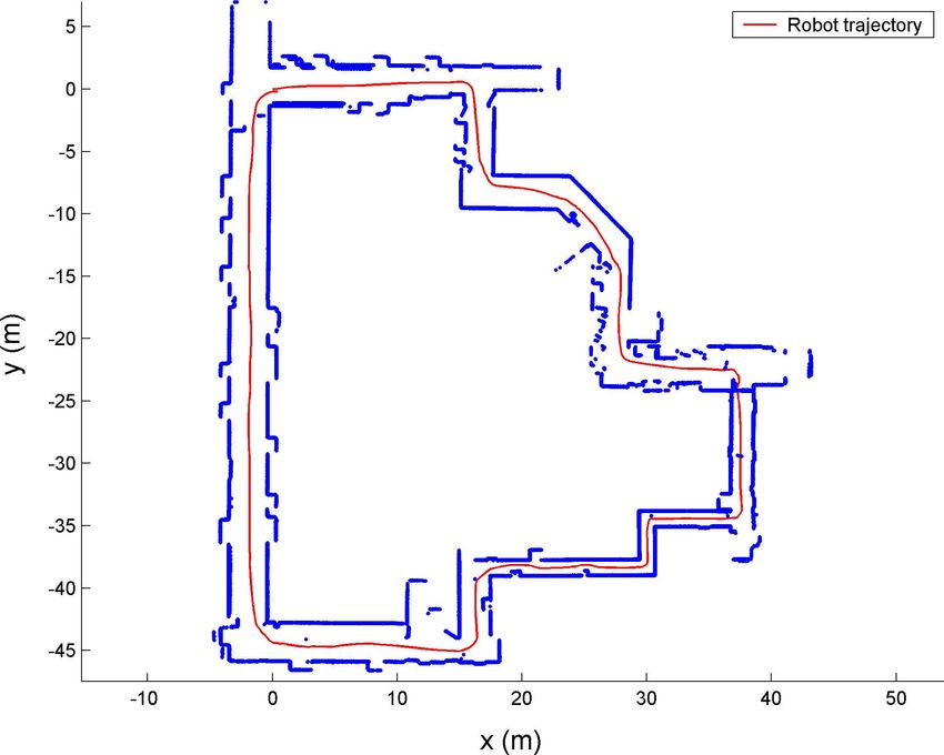
                                           −0.5                                                                                                                                  −0.5                                                                                                             Fig. 4. The estimated trajectory of the robot based only on laser scan matching.
                                                    0               50         100        150         200         250         300     350    400                                          0           50     100              150                            200    250   300   350   400
                                                                                                                                                                                                                                                                                                  The map is presented for visualization purposes only, by transforming all the
                                                                                                 Time (sec)                                                                                                                                        Time (sec)
                                                                                                                                                                                                                                                                                                  laser points using the estimated robot pose.
                                                                                                (c)                                                                                                                                                (d)
                                            6                                                                                                                                     6
                                                            Error                                                                                                                             Error
                                                            ±3σ                                                                                                                               ±3σ

                                            4                                                                                                                                     4

                                                                                                                                                                                                                                                                                                  in significantly smaller values for the covariance of the robot’s
             Orientation error (degrees)

                                                                                                                                                   Orientation error (degrees)

                                            2                                                                                                                                     2
                                                                                                                                                                                                                                                                                                  pose estimates. Based on numerous experiments and simulation
                                            0                                                                                                                                     0                                                                                                               tests, it appears that this is a common result, which indicates
                                           −2                                                                                                                                    −2
                                                                                                                                                                                                                                                                                                  that the correlation between consecutive displacement estimates
                                                                                                                                                                                                                                                                                                  tends to be negative.
                                           −4                                                                                                                                    −4

                                                                                                                                                                                                                                                                                                     An intuitive explanation for this observation can be given by
                                           −6
                                                0              50             100         150         200
                                                                                                Time (sec)
                                                                                                                  250         300     350    400
                                                                                                                                                                                 −6
                                                                                                                                                                                      0          50         100         150                              200
                                                                                                                                                                                                                                                  Time (sec)
                                                                                                                                                                                                                                                                    250   300   350   400         means of a simple example, for motion on a straight line: as
                                                                                                (e)                                                                                                                                                (f)                                            shown in Section III, the correlation of consecutive displace-
                                                                                                                                                                                                                                                                                                  ment estimates is attributed to the fact that the measurement
                Fig. 3. The robot pose errors (solid lines) vs. the corresponding 99, 8%                                                                                                                                                                                                          errors at time step k affect the displacement estimates for
                percentile of their distribution, (dashed lines with circles). The left column                                                                                                                                                                                                    both time intervals [k − 1, k] and [k, k + 1]. Consider a robot
                shows the results for the SC-KF-WC algorithm proposed in this paper, while
                the right one demonstrates the results for the SC-KF-NC algorithm. The
                                                                                                                                                                                                                                                                                                  moving along a straight-line path towards a feature, while
                “dark zones” in the last figures are the result of an intense sawtooth pattern                                                                                                                                                                                                    measuring its distance to it at every time step. If at time-step
                in the robot’s orientation variance. These fluctuations arise due to the very                                                                                                                                                                                                     k the error in the distance measurement is equal to ²k > 0,
                high accuracy of the relative orientation measurements, compared to the low
                accuracy of the odometry-based orientation estimates. (a - b) Errors along the
                                                                                                                                                                                                                                                                                                  this error will contribute towards underestimating the robot’s
                x-axis (c - d) Errors along the y-axis (e - f) Orientation errors.                                                                                                                                                                                                                displacement during the interval [k − 1, k], but will contribute
                                                                                                                                                                                                                                                                                                  towards overestimating the displacement during the interval
                                                                                                                                                                                                                                                                                                  [k, k +1]. Therefore the error ²k has opposite effects on the two
0.12                                                                                                               0.12                                                                                                                   0.45
                                            Exact                                                                                                              Exact                                                                                                                  Exact
                                            No correlations                                                                                                    No correlations                                                                                                        No correlations
                                                                                                                                                                                                                                                                            0.4
                                  0.1                                                                                                                0.1

                                                                                                                                                                                                                                        Orientation covariance (degees )
                                                                                                                                                                                                                                                                           0.35

                                                                                                                                                                                                                                        2
  Covariance along y−axis (m )

                                                                                                                     Covariance along y−axis (m )
 2

                                                                                                                     2
                                 0.08                                                                                                               0.08                                                                                                                    0.3

                                                                                                                                                                                                                                                                           0.25
                                 0.06                                                                                                               0.06
                                                                                                                                                                                                                                                                            0.2

                                 0.04                                                                                                               0.04                                                                                                                   0.15

                                                                                                                                                                                                                                                                            0.1
                                 0.02                                                                                                               0.02
                                                                                                                                                                                                                                                                           0.05

                                   0                                                                                                                  0                                                                                                                      0
                                        0    50       100     150   200         250    300   350   400   450   500                                         0    50       100     150   200      250       300   350   400   450   500                                             0    50       100     150   200         250    300   350   400   450   500

                                                                          Time (sec)                                                                                                         Time (sec)                                                                                                             Time (sec)

                                                                          (a)                                                                                                            (b)                                                                                                                        (c)
Fig. 5. The estimated covariance of the robot’s pose using when the correlation between consecutive measurements is properly accounted for (solid lines) vs.
the covariance estimated when the correlations are ignored (dashed lines). (a) Errors along the x-axis (b) Errors along the y-axis (c) Orientation errors.

displacement estimates, rendering them negatively correlated.                                                                                                                                     [5] F. Lu and E. Milios, “Robot pose estimation in unknown environments
                                                                                                                                                                                                      by matching 2d range scans,” Journal of Intelligent and Robotic Systems:
                                                                           VI. C ONCLUSIONS                                                                                                           Theory and Applications, vol. 18, no. 3, pp. 249–275, Mar. 1997.
                                                                                                                                                                                                  [6] D. Silver, D. M. Bradley, and S. Thayer, “Scan matching for flooded
   In this paper, we have studied the problem of localiza-                                                                                                                                            subterranean voids,” in Proceedings of the 2004 IEEE Conf. on Robotics,
tion using relative-state measurements that are inferred from                                                                                                                                         Automation and Mechatronics (RAM), December 2004.
exteroceptive information. It has been shown, that when the                                                                                                                                       [7] S. T. Pfister, K. L. Kriechbaum, S. I. Roumeliotis, and J. W. Burdick,
                                                                                                                                                                                                      “Weighted range sensor matching algorithms for mobile robot displace-
same exteroceptive sensor measurements are employed for the                                                                                                                                           ment estimation,” in Proceedings of the IEEE International Conference
computation of two consecutive displacement estimates (both                                                                                                                                           on Robotics and Automation, Washington D.C., May 11-15 2002, pp.
forward and backward in time), these estimates are correlated.                                                                                                                                        1667–74.
                                                                                                                                                                                                  [8] P. Torr and D. Murray, “The development and comparison of robust
An analysis of the exact structure of the correlations has                                                                                                                                            methods for estimating the fundamental matrix,” International Journal
enabled us to derive an accurate formula for propagating                                                                                                                                              of Computer Vision, vol. 24, no. 3, pp. 271–300, 1997.
the covariance of the pose estimates, which is applicable in                                                                                                                                      [9] K. Konolige, “Large-scale map-making.” in AAAI National Conference
                                                                                                                                                                                                      on Artificial Intelligence, San Jose, CA, jul 2004, pp. 457–463.
scenarios when the exteroceptive measurements are the only                                                                                                                                       [10] B. D. Hoffman, E. T. Baumgartner, T. L. Huntsberger, and P. S. Shenker,
available source of positioning information. To address the                                                                                                                                           “Improved state estimation in challenging terrain,” Autonomous Robots,
case in which proprioceptive sensor data are also available,                                                                                                                                          vol. 6, no. 2, pp. 113–130, April 1999.
                                                                                                                                                                                                 [11] S. Julier and J. Uhlman, “A non-divergent estimation algorithm in the
we have proposed an efficient EKF-based estimation algorithm,                                                                                                                                         presence of unknown correlations,” in Proceedings of the American
that correctly accounts for the correlations attributed to the                                                                                                                                        Control Conference, vol. 4, 1997, pp. 2369 – 2373.
relative-state measurements. The experimental results demon-                                                                                                                                     [12] R. C. Smith, M. Self, and P. Cheeseman, Autonomous Robot Vehicles.
                                                                                                                                                                                                      Springer-Verlag, 1990, ch. Estimating Uncertain Spatial Relationships in
strate that the performance of the algorithm is superior to                                                                                                                                           Robotics, pp. 167–193.
that of previous approaches [1], while the overhead imposed                                                                                                                                      [13] M. Montemerlo, “Fastslam: A factored solution to the simultaneous
by the additional complexity is minimal. The method yields                                                                                                                                            localization and mapping problem with unknown data association,” Ph.D.
                                                                                                                                                                                                      dissertation, Robotics Institute, Carnegie Mellon University, July 2003.
more accurate estimates, and most significantly, it provides a                                                                                                                                   [14] S. Thrun, Y. Liu, D. Koller, A. Ng, Z. Ghahramani, and H. Durrant-
more precise description of the uncertainty in the robot’s state                                                                                                                                      Whyte, “Simultaneous localization and mapping with sparse extended
estimates, thus facilitating motion planning and navigation.                                                                                                                                          information filters,” International Journal of Robotics Research, vol. 23,
                                                                                                                                                                                                      no. 7-8, pp. 693–716, Aug. 2004.
                                                                    ACKNOWLEDGEMENTS                                                                                                             [15] P. S. Maybeck, Stochastic Models, Estimation, and Control. Academic
                                                                                                                                                                                                      Press, 1979, vol. I.
  This work was supported by the University of Minnesota                                                                                                                                         [16] T. Bailey, “Constrained initialisation for bearing-only SLAM,” in Pro-
(DTC), the Jet Propulsion Laboratory (Grant No. 1251073,                                                                                                                                              ceedigs of the IEEE International Conference on Robotics and Automa-
                                                                                                                                                                                                      tion (ICRA), vol. 2, Sept. 2003, pp. 1966–1971.
1260245, 1263201), and the National Science Foundation (ITR-                                                                                                                                     [17] J. Leonard, R. Rikoski, P. Newman, and M. Bosse, “Mapping partially
0324864, MRI-0420836).                                                                                                                                                                                observable features from multiple uncertain vantage points,” The Inter-
                                                                                                                                                                                                      national Journal of Robotics Research, vol. 21, no. 10-11, pp. 943–975,
                                                                                      R EFERENCES                                                                                                     2002.
                                                                                                                                                                                                 [18] J. Neira and J. D. Tardos, “Data association in stochastic mapping
 [1] S. I. Roumeliotis and J. Burdick, “Stochastic cloning: A generalized                                                                                                                             using the joint compatibility test,” IEEE Transactions on Robotics and
     framework for processing relative state measurements,” in IEEE Interna-                                                                                                                          Automation, vol. 17, no. 6, pp. 890–897, 2001.
     tional Conference on Robotics and Automation, Washington D.C., 2002,                                                                                                                        [19] A. Howard, “Multi-robot mapping using manifold representations,” in
     pp. 1788–1795.                                                                                                                                                                                   Proceedings of the 2004 IEEE International Conference on Robotics and
 [2] A. Kelly, “General solution for linearized systematic error propagation                                                                                                                          Automation, New Orleans, LA, April 2004, pp. 4198–4203.
     in vehicle odometry,” in Proceedings of the IEEE/RSJ International                                                                                                                          [20] S. Pfister, S. Roumeliotis, and J. Burdick, “Weighted line fitting algo-
     Conference on Intelligent Robots and Systems (IROS), Maui, HI, Oct.29-                                                                                                                           rithms for mobile robot map building and efficient data representation,”
     Nov.3 2001, pp. 1938–45.                                                                                                                                                                         in Proceedings of the IEEE International Conference on Robotics and
 [3] L. Matthies, “Dynamic stereo vision,” Ph.D. dissertation, Dept. of Com-                                                                                                                          Automation, Taipei, Taiwan, Sep. 14-19 2003, pp. 1304–1311.
     puter Science, Carnegie Mellon University, 1989.
 [4] H. S. C.F. Olson, L.H. Matthies and M. Maimone, “Robust stereo ego-
     motion for long distance navigation,” in Proceedings of CVPR, 2000, pp.
     453–458.
You can also read