Joint Configuration and Scheduling Optimization of a Dual-Trolley Quay Crane and Automatic Guided Vehicles with Consideration of Vessel Stability ...
←
→
Page content transcription
If your browser does not render page correctly, please read the page content below
sustainability

Article
Joint Configuration and Scheduling Optimization of
a Dual-Trolley Quay Crane and Automatic Guided
Vehicles with Consideration of Vessel Stability
Lijun Yue, Houming Fan * and Chunxin Zhai
 Department of Transportation engineering, Dalian Maritime University, Dalian 116026, China;
 Yuelj11@163.com (L.Y.); cxzhai@dlmu.edu.cn (C.Z.)
 * Correspondence: fhm468@dlmu.edu.cn; Tel.: +86-0411-8472-5868

 Received: 28 November 2019; Accepted: 15 December 2019; Published: 18 December 2019

 Abstract: This study proposes a formulation to optimize operational efficiency of a dual-trolley
 quay crane and automatic guided vehicles (AGVs) to reduce energy consumption at an automated
 container terminal. A two-phase model is used to minimize energy consumption during loading and
 discharging operations, as well as maximize the utilization rate of the AGVs, with consideration of
 relevant constraints such as the capacity of buffers for the quay crane (QC) and yard, the stability of
 vessel, the maximum endurance of an AGV, and the available laytime for handling. We propose a
 constrained partial enumeration strategy to construct quay crane schedules and a genetic algorithm
 to solve the AGV scheduling problem. Finally, Yangshan Phase IV automated container terminal’s
 data is used to verify the validity and applicability of the proposed model. The results of the tests
 provide evidence that the proposed method can improve energy efficiency.

 Keywords: dual-trolley quay crane; AGV scheduling; energy consumption; available laytime;
 vessel stability

1. Introduction
      To date, the London Port, Kawasaki Port, Singapore Port, Hamburg Port, Xiamen Ocean Gate
Container Terminal, Shanghai Yangshan Port, and other ports have successively built automated
container terminals. To remain competitive, in terms of services and prices, some companies and
researchers have focused on optimizing the line’s schedule reliability and the scheduling of handling
equipment in container terminals. Sea Intelligence in Denmark reported in a study, in June 2019, that
the Hyundai merchant ship ranked first on the list, with an average rate of 91.8%. In the shipping
alliance, the 2M0 s schedule reliability is 91.3%, which is the highest, while the Alliance is the lowest
rate, at only 75.4%. In terms of container terminals, increasingly, the emphasis has been on improving
reliability by completing handling operations within laytime. In addition, efforts have been made to
optimize the loading and discharging operations, which accounts for 48.3% of the energy consumption
in a terminal [1]. The sequence of quay crane moves affects the stability and the scheduling of quay
cranes influences the handling time of the ship. The arrival time of the AGV affects the loading and
discharging containers by the quay crane and the yard crane (YC) [2]. Thus, this paper optimizes the
configuration and scheduling of quay cranes and AGVs aiming to reduce energy consumption at an
automated container terminal, with consideration of the reliability and vessel stability.
      There are extensive literatures on the reduction of energy consumption at a seaport. A major
category of container terminal operations includes the quayside operations, which contains two
separate tasks, allocation of berths and quay crane scheduling. For example, Chang [3] proposed
and verified an investigation about the scheduling strategy of berth and quay crane through a case

Sustainability 2020, 12, 24; doi:10.3390/su12010024                       www.mdpi.com/journal/sustainability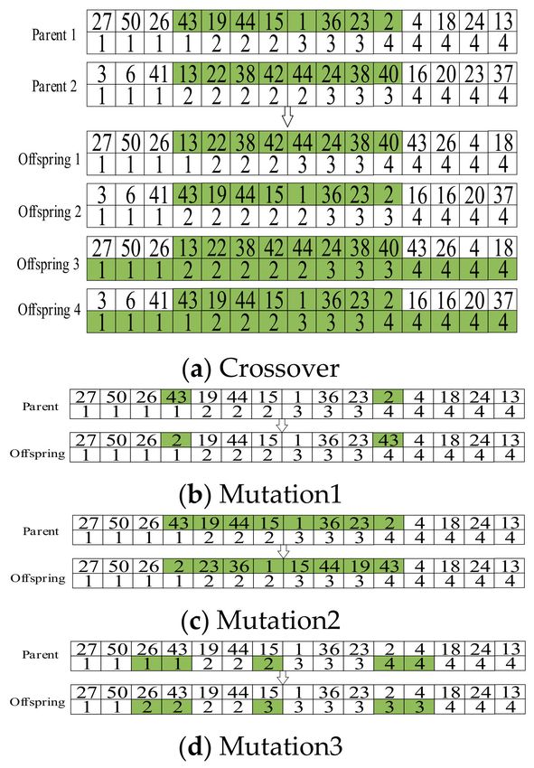
Sustainability 2020, 12, 24                                                                     2 of 16

analysis. He [4] developed a mixed integer model of berth allocation and quay crane allocation with
the goal of minimizing the delay of ships and energy consumption of operations, and solved the
model using the integrated simulation algorithm. Some researchers studied the scheduling of QC
under a known berth plan, with the goal of minimizing makespan among all ships. For example,
Chang [5] studied quay crane scheduling under dynamic ship arrival conditions, and proposed a
dynamic rolling strategy, establishing a model to minimize the handling time of all ships in the port
and balance the quay crane operation. Kovalyov [6] proposed five strategies to optimize the multiple
quay crane scheduling problem of simultaneous loading and discharging operations. Other researchers
have evaluated the effect of quay crane scheduling on reducing energy consumption by viewing
a single container as a group. Liu [7] studied the allocation and scheduling of a quay crane and
established an AGV queuing model with the goal of minimizing CO2 emissions during discharging.
By analyzing the earliest workable time and required completion time of each task, a coupling model
of quay crane scheduling and configuration was established by Liang [8], and used the loop iterative
method to solve the model. Kovalyov [9] proposed an algorithm that included a cutting-plane and
graph-based binary search to solve the exact solution of the quay crane scheduling model, and verified
the effectiveness of the model and algorithm under different sized tasks. Kim [10] established a mixed
integer programming model that considered the priorities of tasks and the safety margin between
quay cranes, and proposed a greedy random adaptive algorithm based on branch and bound to solve
the model. Nguyen [11] used a genetic algorithm and a genetic programming algorithm to solve
the priorities of containers, respectively, to obtain a relatively stable makespan under an uncertain
environment. Zhang [12] established a scheduling model with stability constraints that considered
the ship’s longitudinal stability during loading and discharging, and proposed a heuristic algorithm
based on a sliding window to repair the sequence violating the stability constraints. Al-Dhaheri [13]
developed a model to solve large-scale problems effectively and a Lagrangian relaxation to decompose
problems that were not constrained by stability.
      Another major equipment of container terminal operations is the AGV, which receives the
discharged container from the quay crane and sends it to the yard or delivers the loaded container
from the yard to the quay crane. Regarding the problem of reducing energy consumption of AGV
operations, some researchers have studied the scheduling strategy. For example, Kim [14] aimed to
reduce the delay energy consumption of ships at automated container terminals. Choe [15] proposed
the ONPL (online preference learning) algorithm, which dynamically adjusted the scheduling strategy
of an AGV by updating the preference function. Kim [16] studied the AGV scheduling problem by
considering the multi-standard scheduling strategy. Some researchers have addressed the impact of
the uncertain environment of AGV transportation. For example, Singgih [17] studied the AGV path
planning problem of automated container terminals with consideration of congestion. An integer
programming model was constructed with the objective of minimizing the transiting time and waiting
time of the AGV and solved it using the Dijkstra algorithm. Legato [18] built an optimization model to
minimize the collision time caused by the AGV path conflict, with consideration of the non-constant
efficiency of the quay crane, and solved it using a simulated annealing algorithm.
      More recently, several researchers have adopted integration as a means of simultaneously making
decisions for multiple quay crane and AGV scheduling problems. Xin [19] proposed a two-part
hierarchical control structure, which considered the operation to be continuous dynamics, as well
as discrete dynamics, minimizing the completion time of the upper quay crane and the energy
consumption of the lower layer AGV. Peng [20] quantified the impact of equipment configuration
on carbon emissions, and established a simulation model based on complex queuing networks to
optimize the ratio of the quay crane, the yard crane, and AGVs. On the basis of the hybrid flow
shop scheduling problem (HFSS), Yang [21] proposed the dual-objective joint optimization model
for a quay crane, truck, and yard crane with the goal of minimizing total operation time and energy
consumption. Al-Dhaheri [22] proposed an optimization model aiming at minimizing the makespan
of quay crane and the number of AGVs and solved the model with Cplex. Yang [23] studied the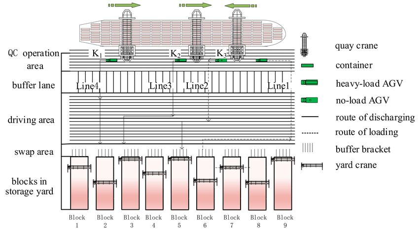
Sustainability 2020, 12, 24                                                                          3 of 16

integrated scheduling of quay crane, AGV, and yard crane for simultaneous loading and discharging
operations, and designed a general algorithm based on preventive congestion rules. Xin [24] proposed
a collision-free scheduling algorithm to generate timetables for AGV, quay crane, and yard crane,
which could reduce the average distance of AGV operation.
     In summary, the above literatures have incorporated either no equipment scheduling decisions
or very simple equipment scheduling decisions in their models. In this study, we propose a model
to optimize the joint configuration and scheduling of a dual-trolley quay crane and AGVs. The
contributions of this study are threefold. First, the effects of available laytime are proposed and
evaluated from the terminal system perspective. Second, the constraints of the buffer platform capacity
of the dual-trolley quay crane and blocks are considered during configuration and scheduling. In
this manner, this study fills the gap in the existing literature, which has evaluated the scheduling of
AGVs only based on known time windows. Third, the utilization of an AGV is improved over the
state-of-the-art in terms of the objective of energy consumption. In addition, this work is the first study
to optimize the joint configuration and scheduling of multiple handling operations.
     The remainder of this paper is organized as follows: Section 2 presents a two-phase model with
the constraint of vessel stability, available laytime, AGV’s endurance time, and buffer platform for
quay crane and blocks. Section 3 describes the enumeration algorithm and genetic algorithm to solve
the problems for seeking a satisfactory solution of AGV and quay crane scheduling. Section 4 proposes
a real case to verify the validity of the model and algorithms and Section 5 summarizes the research
results and proposes future research directions.

2. Problem Description and Mathematical Model

2.1. Problem Description
     The loading and discharging process of an automated container terminal is shown in Figure 1.
During the discharging period, the main trolley of the dual-trolley quay crane places the discharged
container onto the transfer platform, and the gantry trolley takes the container from the transfer
platform and places it on the AGV and, then, the AGV transports the container to the yard and places
the container on the buffer bracket. During the loading period, the no-load AGV takes the loaded
container from the buffer bracket of the yard to the underside of the gantry trolley and, then, the
gantry trolley lifts the container from the AGV onto the transfer platform. When the main trolley
idles, the container on the transfer platform is placed on the ship. In order to minimize the energy
consumption of the loading and discharging operations, the following constraints must be considered
by the dispatching center: available laytime of the ship in port, the stability of the ship, the precedence
of tasks, a safety margin between quay cranes, the buffer size, and the AGV’s endurance.

                  Figure 1. Automated container terminal layout and (AGV) transportation process.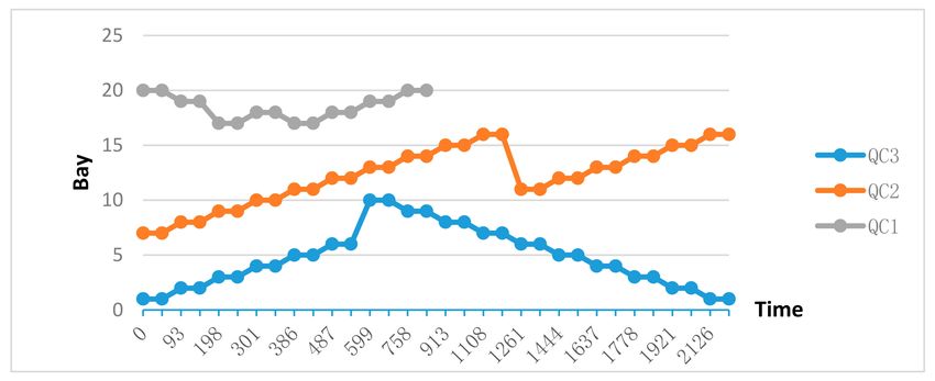
Sustainability 2020, 12, 24                                                                        4 of 16

      In this study, the joint configuration and the scheduling problem of the dual-trolley quay crane
and an AGV in a single-ship operation mode are divided into two phases. In the first phase, the
dual-trolley quay cranes are configured according to the number and location of all containers. A task
is defined as a set of containers to be discharged (loaded) from (at) either the hold or the deck of the
same ship bay. The center of gravity (CG) of ship must be kept within a certain range to meet the
stability requirements. The precedence of the containers is that the discharged container in the hold
is after the container on the deck, and the container on the deck is loaded after the container in the
hold. Container numbering in each bay is based on the precedence relationships between containers.
Figure 2 presents an example for a ship handling loading and discharging containers in six bays. The
tasks are indexed sequentially from discharging containers to loading (bay 1 to bay 6). For example, the
discharged 32 containers in bay 1 is indexed task 1, and the total number of loading and discharging
tasks is 24.

                              Figure 2. Example of containers and tasks on a ship.

     In the second phase, the containers that differ in location need to be distributed from an AGV’s
point of view. One container is a unit during the dispatching process of an AGV. As shown in Figure 1,
after picking up the loaded containers in block 6, the AGV goes to quay crane K3 to deliver the
containers to the ship bay, which the containers belong to. After the loaded containers are released,
the AGV goes to pick up the next loading task in a block of storage areas (Line 2) or operate the next
discharging task under the quay crane K2 (Line 3) or quay crane K1 (Line 4). The AGV stops its
operating cycle to charge when it has a low supply of electricity. A container with a given index must
be handled before all containers with higher indexes located at the same bay. Since the high losses are
caused by the delay of the quay crane, it is necessary to ensure that the main trolley does not wait for
the AGV during handling.
     This study is based on the following assumptions: (1) All containers are of the same type, and all
dual-trolley quay cranes and AGVs have the same performance and fuel consumption, because only
one container(20 ft or 40 ft) can be handled at the same time by the QC or the AGV. (2) The longitudinal
stability of a container ship is considered. (3) Traffic congestion and path conflict of AGVs are not
considered. (4) Buffer size for blocks and QC is considered as given and all automated rail mounted
gantry cranes (ARMGs) have the same performance and fuel consumption.

2.2. Phase I: Mathematical Formulation for Configuration and Scheduling of a Dual-Trolley Quay Crane
      All the sets, parameters, and decision variables of the phase I are shown in Table 1.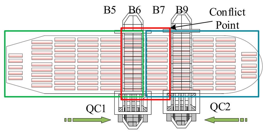
Sustainability 2020, 12, 24                                                                                                                        5 of 16

                                                      Table 1. Parameters of the phase I.

       Sets
                                     represents the set of all tasks, indexed by i, where i is a loading/discharging
       I
                                     operation of the same bay on the deck or hold
       N                             represents the set of all containers, indexed by n
       K                             represents the set of all QCs, indexed by k
       T                             represents the set of time units, indexed by t
       Parameters
       Lsa f e                       safety margin between two consecutive cranes (in number of bays)
       tf                            available laytime of the ship
       G0i                           center gravity of the ship before starting the operations
       Gti                           workload before starting the operations in task i
                                     handled workload at time segment t in task i
       shi f t                       maximum allowable shift with the center gravity of the ship (in number of bays)
       δ                             1 for loading operations; -1 for discharging operations
       ρti                           weight of task i at time segment t
       τ1                            the time required for QCs to move a bay in the direction of the ship
       τ2                            the average time required for the QCs to pick up and release a container
       c1                            unit time energy consumption for QC loading and discharging
       c2                            unit time energy consumption for QC moving
       c3                            unit energy consumption for QC waiting
       Ni                            workload in number of containers at tasks i
       li                            location of task (in ship-bay number)
                                     the time that the QC k needs to waiting before starting the task j after the
       wijk
                                     completed task i
       Decision variables            (
                                       1                                           if QC k performs task i at time segment t
       xtik
                                     ( 0                                           Otherwise
       xijk                            1                                           If QC k performs task j after performing task i
                                       0                                           Otherwise

    Object 1: Minimize the total energy consumption of QCs which includes working energy
consumption, moving energy consumption, and waiting energy consumption.

                              T X
                              X I X
                                  K                                           I X
                                                                              X I X
                                                                                  K                                     I X
                                                                                                                        X I X
                                                                                                                            K
           min f1 = C1 ×                        xtik Ni τ2 + C2 ×                            l j − li ×xijk τ1 + C3 ×                  xijk wijk      (1)
                              t=1 i=1 k =1                                    i=1 j=1 k =1                              i=1 j=1 k =1

s.t.
                                                                 K
                                                                 X
                                                                        xtik = 1∀i ∈ I, t ∈ T                                                         (2)
                                                                 k =1
                                                                 T X
                                                                 X K
                                                                               xtik = Ni ∀i ∈ I                                                       (3)
                                                                 t=1 k =1

                                                     I
                                                     X               I
                                                                     X
                                                            xijk −            x jik = 0∀i ∈ I, ∀k ∈ K                                                 (4)
                                                      j=1               j=1

              T X
              X I X
                  K                           X I X
                                              K X I                                      K X
                                                                                         X I X
                                                                                             I
                             xtik Ni τ2   +                      l j − li ×xijk τ1 +                    xijk wijk ≤ t f ∀i, j ∈ I, ∀k ∈ K             (5)
              t=1 i=1 k =1                    k =1 j=1 i=1                               k =1 j=1 i=1

                                               I
                                               X                 I
                                                                 X
                                                     xtik li −          xtjk0 l j ≥ Lsa f e ∀k, k0 ∈ K, t ∈ T                                         (6)
                                               i=1               j=1
Sustainability 2020, 12, 24 6 of 16
I
(δGti + G0i )ρti (li − 21 )
P
i=1
g0 − shi f t ≤ ≤ g0 + shi f t∀t ∈ T (7)
I
(δGti + G0i )ρti
P
i=1
xik , xijk ∈ {0, 1}∀i, j ∈ I, ∀k ∈ K (8)
Constraint (2) ensures that each task is performed by one QC. Constraint (3) guarantees that all
containers workload will be handled. Constraint (4) guarantees that each task has one and only one
predecessor task and a dummy task. Evidently, the largest time required to service all tasks cannot
exceed the available laytime, which is ensured through constraint (5). Constraint (6) enforces the
safety margin between QCs. Constraint (7) ensures that the shift of a ship’s center of gravity must be
maintained within acceptable limits. Finally, the binary nature of the decision variable is specified by
constraint (8).
2.3. Phase II: Mathematical Formulation for AGV Scheduling
The handling time of containers by the QC can be obtained through the first phase. In this
part, loaded and discharged containers are assigned to each AGV and the sequence of operations
is scheduled while ensuring that no quay crane is delayed. All the sets, parameters, and decision
variables are shown in Table 2.
Table 2. Parameters of the phase II.
Sets
L represents the set of loaded containers
D represents the set of discharged containers
C represents the set of yard cranes(YCs), indexed by c
A represents the set of AGVs, indexed by a
Parameters:
q
Tnk planned handling time of the nth container by main trolley of quay crane k
e
Tnk planned handling time of the nth container by gantry trolley of quay crane k
Snc planned handling time of the nth container by the yard crane c
ETnkO earliest starting time of quay crane k for container n
LTnko
latest starting time of quay crane k for container n
ETncG earliest starting time of yard crane c for container n
LTncG latest starting time of yard crane c for container n
C4 unit time waiting energy consumption for gantry trolley of QC
C5 unit time energy consumption for AGV convey containers.
C6 unit time moving energy consumption for no-load AGV
C7 unit time waiting energy consumption for AGV
p1 size of transit platform of on dual-trolley quay crane
p2 size of buffer bracket in each block
τ3 the time required for QC to pick up/put down a container
τ4 the time required for yard crane to pick up/put down a container
τ5 the time required for AGV to make a round trip to the charging station
v1 speed of load AGV
v0 speed of no-load AGV
Q
Tnk actual handling time of the nth container by main trolley of quay crane k
E
Tnk actual handling time of the nth container by gantry trolley of quay crane k
Decision variables (
1 if container n is assigned by the ath AGV.
xna
( 0 Otherwise
1 if ath AGV performs container n0 after performing container n
xnn0a
0 Otherwise
if ath AGV’s power is less than the safe power after
una
1
performing container n
Otherwise
0
Sustainability 2020, 12, 24 7 of 16
The objective is to minimize the energy consumption of the schedule in order to increase the
utilization rate of AGVs.
K P
N A P
N A P
N P
N
E − Te ) + C ×
P P P
f2 = C4 × (Tnk nk 5 xna tna + C6 × xnn0 a tnn0 a
k =1 n=1 a=1 n=1 a = 1 n0 = 1 n = 1
A P
C P
N A P
K P
N (9)
P P
+C7 × ( wnca + wnka )
a=1 c=1 n=1 a=1 k =1 n=1
s.t.
A
X
xna = 1 ∀n ∈ N (10)
a=1
N
X
x0nk = 1 ∀k ∈ K (11)
n=1
N
X
xnωk = 1 ∀k ∈ K (12)
n=1
Q q
Tnk ≤ Tnk ∀n ∈ N (13)
O q O q
ETnk = Tnk − p1 × τ2 , LTnk = Tnk ∀n ∈ L, ∀k ∈ K (14)
O q O q
ETnk = Tnk , LTnk = Tnk + p1 × τ2 ∀n ∈ D, ∀k ∈ K (15)
O E 1 O
ETnc ≤ Tnk + τ3 ≤ LTnc ∀n ∈ L, ∀k ∈ K (16)
2
O E 1 O
ETnc ≤ Tnk − τ3 ≤ LTnc ∀n ∈ D, ∀k ∈ K (17)
2
n o
E e
Tnk = max Tna , Tnk ∀n ∈ D, ∀k ∈ K, ∀a ∈ A (18)
n o
E e
Tnk = max Tna + tna , Tnk ∀n ∈ L, ∀k ∈ K, ∀a ∈ A (19)
Tne 0 k = Tnk
E
+ τ3 ∀n, n0 ∈ N, ∀k ∈ K (20)
G G
ETnc = Snc , LTnc = Snc + p2 × τ4 ∀n ∈ L, ∀c ∈ C (21)
G G
ETnc = Snc − p2 × τ4 , LTnc = Snc ∀n ∈ D, ∀c ∈ C (22)
G G
ETnc ≤ Tna ≤ LTnc ∀n ∈ L, ∀a ∈ A, ∀c ∈ C (23)
G G
ETnc ≤ Tna + tna ≤ LTnc ∀n ∈ D, ∀a ∈ A, ∀c ∈ C (24)
n o
e
wnka = max Tnk − Tna − tna , 0 ∀n ∈ L, ∀k ∈ K, ∀a ∈ A (25)
n o
e
wnka = max Tnk − Tna , 0 ∀n ∈ D, ∀k ∈ K, ∀a ∈ A (26)
n o
G
wnca = max ETnc − Tna , 0 ∀n ∈ L, ∀a ∈ A, ∀c ∈ C (27)
n o
G
wnca = max ETnc − Tna − tna , 0 ∀n ∈ D, ∀a ∈ A, ∀c ∈ C (28)
Tna + tna + wnka + tnn0 a + wn0 ca + τ5 × una ≤ Tn0 a + M(1 − xnn0 a ) ∀n ∈ L, n0 ∈ L (29)
Tna + tna + wnka + tnma + wn0 ka + τ5 × una ≤ Tn0 a + M(1 − xnn0 a ) ∀n ∈ L, n0 ∈ D (30)
Tna + tna + wnca + tnn0 a + wn0 ka + τ5 × una ≤ Tn0 a + M(1 − xnn0 a ) ∀n ∈ D, n0 ∈ L (31)
Tna + tna + wnca + tnn0 a + wn0 ka + τ5 × una ≤ Tn0 a + M(1 − xnn0 a ) ∀n ∈ D, n0 ∈ D (32)Sustainability 2020, 12, 24 8 of 16
A P
P N
C5 × xna tna
a=1 n=1
µ= (33)
A P
P N A P
P N P
N A P
P C P
N A P
P K P
N
C5 × xna tna + C6 × xnn0 a tnn0 a + C7 × ( wnca + wnka )
a=1 n=1 a = 1 n0 = 1 n = 1 a=1 c=1 n=1 a=1 k =1 n=1
xna , xnn0 a , una ∈ {0, 1}∀n, n0 ∈ N, ∀a ∈ A (34)
Tna ≥ 0∀n ∈ N, ∀a ∈ A (35)
Constraint (10) ensures that each container is served by one AGV. Constraints (11) and (12) imply
that each AGV has a starting point and destination. Constraint (13) enforces that the main trolley of
the quay crane is not delayed. The time window is determined in constraints (14) and (15) by each QC
according to the first phase results. Constraints (16) and (17) ensure that each container is served by
quay crane under the time windows. The actual handling time of the nth container by quay crane is
determined in constraints (18) and (19). Constraint (20) specifies the updated plan handling time of the
gantry trolley of the quay crane. The actual handling time of the nth container by the yard crane is
determined in constraints (21) and (22). Constraints (23) and (24) ensure that each container is served
by a yard crane under the time windows. Constraints (25) to (28) imply the waiting time when the AGV
arrives early. Constraints (29) to (32) determine the starting time of the next container by one AGV. The
utilization is calculated by Constraint (33). Constraints (34) and (35) restrict the domains of variables.
3. Algorithms
In this section, we present two algorithms for the configuration and scheduling optimization
model of the quay crane and AGV.
3.1. Enumeration Algorithm for Solving the First Phase Model
Similar to quay crane scheduling with the non-interference constraints problem (QCSNIP) [25]
and the three-dimensional knapsack problem with balancing constraints [26], all tasks must be handled
during the laytime and the center of ship must lie into a predefined bayed domain inside the ship.
Moreover, Lee [25] proved that the QCSNIP is NP-complete and that no polynomial time algorithm
for the exact solution exists. Therefore, in this case, the enumeration algorithm (EA) is proposed for
solving the quay crane configuration and scheduling problem with laytime, precedence, safety margin,
and stability constraints as described in following steps:
(1) Generation of task assignment matrices of each quay crane
Arrange all tasks according to the precedence as follows: Tasks with a smaller ship bay number
are placed first when two tasks of different bays are served by the same quay crane; the task of an
on-deck container is earlier than an in-hold container when two discharging tasks of the same bay are
served by the same quay crane, and vice versa. The enumeration algorithm is employed to generate
the initial task assignment matrices of each quay crane.
To keep the ship stable, the first quay crane moves from the bow to the stern, and the last quay
crane moves from the stern to the bow. As shown in Figure 3, QC 1 moves from left to right, and bay 6
belongs to the task assignment matrices of QC 1. QC 2 moves from right to left, and bay 7 belongs to
the QC 2’s work area. In order to reduce the waiting time of the quay crane at the conflict point, the
avoidance strategy is adopted, which means that QC 1 can handle bay 6 in advance, and then return to
bay 5.Sustainability 2020, 12, 24 9 of 16
Figure 3. Example of a possible conflict point.
(2) Traversing the set of feasible solutions for the optimal scheduling scheme.
We use a constrained partial enumeration strategy to remove the infeasible solution. Calculating
the makespan and stability of the vessel, distance between quay cranes over time, and only keeping
schemes that meet the constraints (5) to (7). The scheduling scheme with the minimum objective value
are retained.
(3) Determining the optimal configuration scheme.
The optimal configuration was obtained by comparing the values of objectives under the different
number of quay cranes configured.
3.2. Extended Genetic Algorithm for Solving the Second Phase Model
Since it is very complex and time consuming to explore the whole solution space, we extended
the genetic algorithm to solve the second phase model. The genetic algorithm has the advantage of
flexibility and imposes no requirement for a problem to be formulated as any particular type. Thus,
they can be applied to non-liner problems for which there is a way to encode the quality of a solution.
Here, we use an integer chromosomal representation. The algorithm consists of five parts as follows:
(1) Chromosome representation
A chromosome is represented by a matrix with 2 × n genes. The gene value in the first line of
chromosome represents the number of containers, and the gene value in the second line represents the
number of AGVs assigned to each container. According to the stowage plan and the distribution results
of the quay crane in the first phase, the number of quay crane and yard crane for each container can be
obtained. Figure 4 illustrates an example of a chromosome with 3 QCs, 4 AGVs and 15 containers. The
container 27 is operated by yard crane 7 and quay crane 2, assigned to AGV 1 for transportation.
Figure 4. The chromosome.
(2) Generating initial population
The initial population can be generated randomly or heuristically. Random generation gives the
initial population great diversity. A population of individuals is initialized by randomly selecting tasks
with the constraints (10) to (12) to make sure every solution is feasible.
(3) Fitness evaluation and chromosomal selection
The chromosomes with high fitness are selected and proceed to the next iteration. Figure 5 shows
the procedure to calculate the objective value. After the generation of a population, its fitness valueSustainability 2020, 12, 24 10 of 16
should be higher. Hence, the reciprocal value of the objective function is taken as the fitness value and
chromosomes with the higher fitness values have a greater chance to survive.
Figure 5. Flowchart for solving the model.
(4) Crossover and mutation
Grouping the chromosomes (individuals) of a population into groups of eight. The parent
chromosomes taken from the groups with the highest value are retained for the next generation.
Figure 6 presents the produced offsprings from two parent chromosomes. A two-point crossover is
used to produce new chromosomes in which the workload of each containers is fully shared between
AGVs. The position of the intersection point is randomly generated. The new offsprings are depicted
in Figure 6a. These crossovers are applied to generate two cross children per chromosome.
The mutation is achieved by varying the index or number of containers served by each AGV and
varying the index of AGVs to containers. We adopt three common types of mutation referred to as
swap and insert. The specific changes of the mutation operation are shown in Figure 6b–d. These
mutations are applied to parent chromosomes generating three mutated children chromosomes.Sustainability 2020, 12, 24 11 of 16
Figure 6. Crossover and mutation.
(5) Stopping criterion
The GA algorithm terminates when the algorithm reaches the maximum number of iterations.
4. Case Studies
4.1. Experimental Setting
The numerical tests in this section are conducted on a server Intel (R) Core(TM) i7-7700 CPU@
3.6GHz with the memory of 16.00GB. The real data comes from Shanghai Yangshan Phase IV automated
container terminal located in China, which has high throughput. The layout of the terminal and
the traffic rules for horizontal transportation are shown in Figure 1. The positional distribution of
containers on the ship presented in [13] is shown in Figure 7, and there are 20 bays waiting for loading
or discharging. The configuration of dual-trolley quay crane + AGV + automated rail mounted gantry
crane (ARMG) is adopted in the research, and some of relevant parameters of quay crane and AGV,
such as travelling speed and operating energy consumption [27,28], are shown in Table 3.
Figure 7. Number of loaded and discharged containers of ship.Sustainability 2020, 12, 24 12 of 16
Table 3. Device-related parameter values.
Parameters Value Parameters Value
τ1 /min 1 C1 /[kw · h] 91.24
τ2 /min 2 C2 /[kw · h] 70.18
τ3 /min 1 C3 /[kw · h] 49.6
τ4 /min 3 C4 /[kw · h] 49.6
C5 /[kw · h ·
τ5 /min 5 21
vch−1 ]
C6 /[kw · h ·
v1 /[m · min−1 ] 210 14
vch−1 ]
C7 /[kw · h ·
v0 /[m · min−1 ] 350 9
vch−1 ]
There are nine blocks in the container yard for stacking containers waiting to be discharged and
loaded. The capacity of the transfer platform of dual-trolley quay crane is set to two containers, and
the safety margin between two quay cranes is set to one bay. The capacity of buffer bracket of each
block is set to five containers. An AGV can last 480 minutes after the battery is replaced.
4.2. Optimization Results
4.2.1. The Results of Quay Crane Scheduling and Configuration in the First Phase
The calculation process is coded in Matlab2016. In all instances, the permitted shift of the vessel’s
CG is assumed to be two bay lengths. The laytime of the ship is assumed to be 44 h. In this test, two
quay cranes cannot help to complete within 44 h. When the number of cranes is 3 or 4, the makspan
was below the laytime limit, however, the energy consumption and time consumption of the latter
was higher than the former for the reason that waiting energy consumption increased. Therefore, the
optimal number of quay cranes is three, the minimum energy consumption of quay cranes is 10,024
kw · h, and the makespan is 2577 min. The optimal scheduling scheme is as follows: For the discharging
operation, QC1 is responsible for bays 1 to 6, QC2 is responsible for bays 7 to 16, and QC3 discharges
bays 17 to 20; for the loading operation, QC1 is responsible for bays 1 to 10, QC2 is responsible for bays
11 to 16, and QC3 loads bays 17 to 20. Figure 8 reports the obtained results. QC1 finished discharging
operation and started loading operation at the 599th min, and QC3 finished discharging operation at
the 1369th min. The synchronous operation time was 770 min, which was conducive to reducing the
AGV’s no-load time. A safety margin between two consecutive cranes is maintained at any time with
no intersection of the moving routes.
Figure 8. Path to the dual-trolley quay cranes.Sustainability 2020, 12, 24 13 of 16
4.2.2. The Results of AGV Scheduling and Configuration in the Second Phase
In the second phase, 3769 containers are considered. On the basis of the results of first phase,
coding genetic algorithm framework with MATLAB is used to obtain the AGV scheduling schemes.
On the basis of the preliminary tests, the population size, the probability of crossover, the probability
of mutation, and the maximum number of generations are set to 120, 0.8, 0.2, and 1500, respectively.
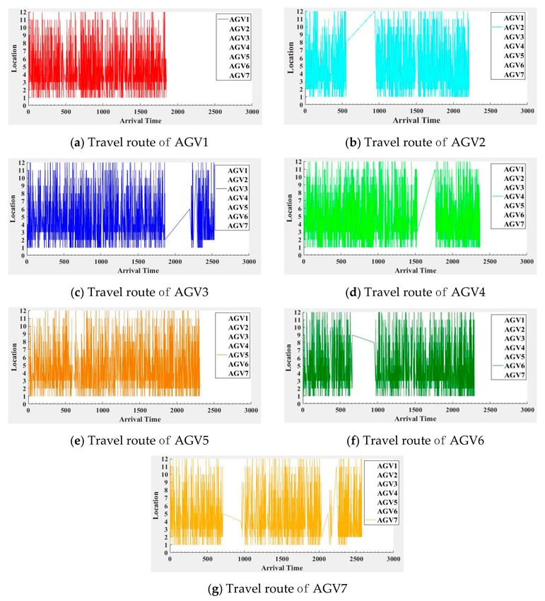
The total energy consumption of seven AGVs is 3202.4 kw · h, and the utilization rate of the AGVs is
55.5%. The scheduling schemes of the AGVs are shown in Figure 9a–g.
Figure 9. The travel route of AGVs.
In order to verify the effectiveness of the model and algorithm, we illustrate the comparison of
these strategies, in terms of laytime of ships and configuration principles of an AGV. The comparison is
shown in Table 4 where principle 1 is minimum energy consumption, principle 2 is minimum number
of AGV configured, and principle 3 is set configure ratio of quay cranes and AGVs with 1:3 mentioned
in [29]. We can see that the shorter the laytime is the more quay cranes need to be configured. For the
same number of QCs, the energy consumption increased when the laytime decreased.Sustainability 2020, 12, 24 14 of 16
Table 4. The results of different laytime and different AGV configuration principles.
Text tf /h Tqmax /h
K/
f1 /kw·h min(f1 +f2 ) Principle 1 Principle 2 Principle 3
piece /kw·h V/vch f2 /kw·h V/vch f2 /kw·h V/vch f2 /kw·h
1 48 / 2 / / / / / / / /
2 44 42.95 3 10,024.4 13226.8 7 3202.4 6 3269.8 9 3548.8
3 40 38.60 3 10,058.2 13377.6 7 3319.4 7 3319.4 9 3594.5
4 36 34.11 4 10,180.9 13450.3 8 3269.4 8 3269.4 12 3515.8
5 32 31.53 4 10,180.9 13429.8 8 3248.9 7 3414.2 12 3459.6
Figure 10 depicts the utilization rates of AGVs with different configuration principles. In all tests,
the third principle has the lower utilization rate. For example, in test 2 where nine AGVs are assigned
to three QCs, the utilization rate is as low as 54%. This indicates that a large number of AGVs cannot
decrease energy consumption, and a good planning coordination technique is necessary. The second
principle is not competitive because it can result in a high utilization for each AGV and high total
energy consumption with quay crane delayed. The first principle saves a significant percentage of the
number of AGVs without any delay, under the decoupling effect of the transit platform of dual-trolley
quay crane and the buffer bracket at storage yard. For example, in test 5 where seven AGVs are
assigned to four QCs the ratio rose to 1:1.75. As compared with principle 3, the first principle has
shorter waiting time for AGVs, for example, in test 2 where seven AGVs are assigned to three QCs, the
energy consumption is reduced 10.8%.
Figure 10. The utilization rate of AGV.
5. Conclusions
In this paper, we have discussed a method for joint configuration and scheduling optimization of a
dual-trolley quay crane and AGVs. The problem has introduced as a scheduling problem with stability
constraints, available laytime constraints, precedence constraints, safety margin constraints, buffer size
constraints, and AGVs’ endurance time constraints. A two-phase optimization model is established, in
which the optimization goal of the first phase is to minimize the energy consumption of the dual-trolley
quay crane, and that of the second phase is to minimize the energy consumption and maximize the
utilization rate of the AGVs. The EA algorithm is used to calculate the working time of the main trolley
for each container. The improved genetic algorithm is used to solve the second-phase model, and the
optimal operation sequence of AGV can be obtained without main trolley delay. Furthermore, the
effectiveness of the model and algorithm is verified by analyzing and comparing the dual-trolley quay
crane and AGV configuration and scheduling schemes under different available laytimes and different
AGV configuration principles. The research in this study resulted in the following conclusions:
(1) A two-phase mixed integer programming model is proposed. The enumeration algorithm is
developed to solve the quay crane scheduling, and the genetic algorithm is improved to obtainSustainability 2020, 12, 24 15 of 16
the AGV scheduling, in order to complete the loading and discharging operations of all containers
on the ship and maintain the stability of the ship in laytime.
(2) The available laytime has an impact on the configured number of quay cranes. The shorter the
laytime, the more the quay cranes are configured, and the more total energy consumption of the
handling operations. The stability has an impact on the movement sequence of the quay cranes.
The order of operations can be changed to reduce the wait time of the quayside and keep the
ship stable.
(3) The single ship’s operation and scheduling mode has been studied by converting the buffer
platform of the dual-trolley quay crane and the buffer bracket of block constraints into time
window constraints. According to the results of this experiment, it was found that the ratio of
quay cranes and AGVs after optimization is about 1:2, which is higher than the optimal ratio
1:3 obtained by a simulation in the study by [29]. Regardless of the influence of an uncertain
environment and other factors, in case 5, the configuration ratio of quay cranes and AGV was
1:1.75, without delay of the main trolley. However, because of the energy consumption caused by
the waiting of quay cranes and yard cranes, the energy consumption of the handling operation
could not be lowest.
This research is more in line with the actual loading and discharging process at an automated
container terminal, but there are still some shortcomings. This paper did not consider the uncertain
factors in the loading and discharging process, such as the path conflict and congestion, which affect
the handling time of containers in the actual environment. By changing the input value, such as the
speed of the AGV or the efficiency of the QC in the model, from deterministic to indeterminate, the
problem of quay crane and AGV joint scheduling affected by uncertain factors could be the future
research direction.
Author Contributions: Conceptualization, L.Y. and H.F.; methodology, L.Y. and H.F.; software, L.Y.; validation,
L.Y. and H.F. case study, L.Y. and H.F.; investigation, L.Y.; resources, H.F.; data curation, L.Y.; writing—original
draft preparation, L.Y. and C.Z.; writing—review and editing, H.F.; supervision, H.F.; project administration, H.F.
All authors have read and agreed to the published version of the manuscript.
Funding: This research was funded by National Natural Science foundation of China (no. 61473053), the project
of Double First-Class Construction (Innovative Projects) (no. CXXM2019SS013).
Conflicts of Interest: The authors declare no conflict of interest.
References
1. Sim, J. A carbon emission evaluation model for a container terminal. J. Clean. Prod. 2018, 186, 526–533.
[CrossRef]
2. He, J.; Huang, Y.; Yan, W. Yard crane scheduling in a container terminal for the trade-off between efficiency
and energy consumption. Adv. Eng. Inf. 2015, 29, 59–75. [CrossRef]
3. Chang, D.; He, J.; Bian, Z. An investigation into berth and quay crane scheduling for container terminals
based on knowledge. In Proceedings of the 2010 International Conference on Future Information Technology
and Management Engineering, Changzhou, China, 9 October 2010; pp. 63–66.
4. He, J. Berth allocation and quay crane assignment in a container terminal for the trade-off between time-saving
and energy-saving. Adv. Eng. Inf. 2016, 30, 390–405. [CrossRef]
5. Chang, D.; Fang, T.; Fan, Y. Dynamic rolling strategy for multi-vessel quay crane scheduling. Adv. Eng. Inf.
2017, 34, 60–69. [CrossRef]
6. Kovalyov, M.Y.; Pesch, E.; Ryzhikov, A. A note on scheduling container storage operations of two non-passing
stacking cranes. Networks 2018, 71, 271–280. [CrossRef]
7. Liu, D.; Ge, Y.E. Modeling assignment of quay cranes using queueing theory for minimizing CO2 emission
at a container terminal. Transp. Res. Part D Transp. Environ. 2018, 61, 140–151. [CrossRef]
8. Liang, C.; Fan, L.; Xu, D.; Ding, Y.; Gen, M. Research on coupling scheduling of quay crane dispatch and
configuration in the container terminal. Comput. Ind. Eng. 2018, 125, 649–657. [CrossRef]Sustainability 2020, 12, 24 16 of 16
9. Msakni, M.K.; Diabat, A.; Rabadi, G.; Al-Salem, M.; Kotachi, M. Exact methods for the quay crane scheduling
problem when tasks are modeled at the single container level. Comput. Oper. Res. 2018, 99, 218–233.
[CrossRef]
10. Kim, K.H.; Park, Y.M. A crane scheduling method for port container terminals. Eur. J. Oper. Res. 2004, 156,
752–768. [CrossRef]
11. Nguyen, S.; Zhang, M.; Johnston, M.; Tan, K.C. Hybrid evolutionary computation methods for quay crane
scheduling problems. Comput. Oper. Res. 2013, 40, 2083–2093. [CrossRef]
12. Zhang, Z.; Liu, M.; Lee, C.Y.; Wang, J. The quay crane scheduling problem with stability constraints. IEEE
Trans. Autom. Sci. Eng. 2018, 15, 1399–1412. [CrossRef]
13. Al-Dhaheri, N.; Diabat, A. A Lagrangian relaxation-based heuristic for the multi-ship quay crane scheduling
problem with ship stability constraints. Ann. Oper. Res. 2017, 248, 1–24. [CrossRef]
14. Kim, K.H.; Bae, J.W. A look-ahead dispatching method for automated guided vehicles in automated port
container terminals. Transp. Sci. 2004, 38, 224–234. [CrossRef]
15. Choe, R.; Kim, J.; Ryu, K.R. Online preference learning for adaptive dispatching of AGVs in an automated
container terminal. Appl. Soft Comput. 2016, 38, 647–660. [CrossRef]
16. Kim, J.; Choe, R.; Ryu, K.R. Multi-objective optimization of dispatching strategies for situation-adaptive
AGV operation in an automated container terminal. In Proceedings of the 2013 Research in Adaptive and
Convergent Systems, Montreal, QC, Canada, 1–4 October 2013.
17. Singgih, I.K.; Hong, S.; Kim, K.H. Flow Path Design for Automated Transport Systems in Container Terminals
Considering Traffic Congestion. Ind. Eng. Manag. Syst. 2016, 15, 19–31. [CrossRef]
18. Legato, P.; Mazza, R.M.; Trunfio, R. Simulation-based optimization for discharging/loading operations at a
maritime container terminal. OR Spectrum 2010, 32, 543–567. [CrossRef]
19. Xin, J.; Negenborn, R.R.; Lodewijks, G. Energy-aware control for automated container terminals using
integrated flow shop scheduling and optimal control. Transp. Res. Part C Emerg. Technol. 2014, 44, 214–230.
[CrossRef]
20. Peng, Y.; Wang, W.; Liu, K.; Li, X.; Tian, Q. The Impact of the allocation of facilities on reducing carbon
emissions from a green container terminal perspective. Sustainability 2018, 10, 1813. [CrossRef]
21. Yang, Y.; Zhu, X.; Haghani, A. multiple equipment integrated scheduling and storage space allocation
in rail–Water intermodal container terminals considering energy efficiency. Transp. Res. Rec. 2019, 2673,
199–209. [CrossRef]
22. Dkhil, H.; Yassine, A.; Chabchoub, H. Optimization of container handling systems in automated maritime
terminal. In Advanced Methods for Computational Collective Intelligence; Springer: Berlin/Heidelberg, Germany,
2013; pp. 301–312.
23. Yang, Y.; Zhong, M.; Dessouky, Y.; Postolache, O. An integrated scheduling method for AGV routing in
automated container terminals. Comput. Ind. Eng. 2018, 126, 482–493. [CrossRef]
24. Xin, J.; Negenborn, R.R.; Corman, F.; Lodewijks, G. Control of interacting machines in automated container
terminals using a sequential planning approach for collision avoidance. Transp. Res. Part C Emerg. Technol.
2015, 60, 377–396. [CrossRef]
25. Lee, D.H.; Wang, H.Q.; Miao, L. Quay crane scheduling with non-interference constraints in port container
terminals. Transp. Res. Part E Logist. Transp. Rev. 2008, 44, 124–135. [CrossRef]
26. Baldi, M.M.; Perboli, G.; Tadei, R. The three-dimensional knapsack problem with balancing constraints. Appl.
Math. Comput. 2012, 218, 9802–9818. [CrossRef]
27. Luo, X. Comparison of horizon transportation system of full automatic container terminal. Port Waterw. Eng.
2016, 9, 76–82.
28. Chen, C.; Zhang, Z.; Zeng, Q.C. Integrated scheduling model of mixed cross-operation for container terminal.
J. Traffic Transp. Eng. 2012, 3, 92–100.
29. Han, X.; Fan, J. Analysis of AGV dispatching and configuration simulation of automated container terminals.
J. Chongqing Jiaotong Univ. 2016, 35, 151–154, 164.
© 2019 by the authors. Licensee MDPI, Basel, Switzerland. This article is an open access
article distributed under the terms and conditions of the Creative Commons Attribution
(CC BY) license (http://creativecommons.org/licenses/by/4.0/).You can also read