Traffic Congestion Aware Route Assignment - DROPS
←
→
Page content transcription
If your browser does not render page correctly, please read the page content below
Traffic Congestion Aware Route Assignment
Sadegh Motallebi
The University of Melbourne, Australia
s.motallebi@student.unimelb.edu.au
Hairuo Xie
The University of Melbourne, Australia
xieh@unimelb.edu.au
Egemen Tanin
The University of Melbourne, Australia
etanin@unimelb.edu.au
Kotagiri Ramamohanarao
The University of Melbourne, Australia
kotagiri@unimelb.edu.au

      Abstract
Traffic congestion emerges when traffic load exceeds the available capacity of roads. It is challenging
to prevent traffic congestion in current transportation systems where vehicles tend to follow the
shortest/fastest path to their destinations without considering the potential congestions caused by
the concentration of vehicles. With connected autonomous vehicles, the new generation of traffic
management systems can optimize traffic by coordinating the routes of all vehicles. As the connected
autonomous vehicles can adhere to the routes assigned to them, the traffic management system
can predict the change of traffic flow with a high level of accuracy. Based on the accurate traffic
prediction and traffic congestion models, routes can be allocated in such a way that helps mitigating
traffic congestions effectively. In this regard, we propose a new route assignment algorithm for the
era of connected autonomous vehicles. Results show that our algorithm outperforms several baseline
methods for traffic congestion mitigation.

2012 ACM Subject Classification Information systems → Geographic information systems

Keywords and phrases Road Network, Traffic Congestion, Route Assignment, Shortest Path

Digital Object Identifier 10.4230/LIPIcs.GIScience.2021.I.9

 1      Introduction
Traffic congestion has significant negative impact on the economy and public health in many
countries. For example, road users in the United States wasted at least 6.9 billion hours and
3.1 billion gallons of fuel in a recent year due to traffic congestions [19]. Traffic congestion
generally appears when traffic demand for certain roads exceeds the available capacity of
the roads. During a traffic congestion, the speed of vehicles reduces, leading to longer travel
times. Statistics show that traffic congestions affect the central area of a city more than the
surrounding suburbs [23].
    Navigating vehicles with the optimized routes can reduce traffic congestion significantly [11,
15, 3]. However, existing approaches are focused on vehicle-level route optimizations where
individual vehicle routes are optimized independent to each other. The next generation of
vehicles, connected autonomous vehicles (CAVs), can drive with the minimal need for human
driver’s intervention. Based on our traffic management vision [17], such vehicles bring a
valuable opportunity to build a coordinated traffic management system (TMS) that can
optimize traffic at the network-level for all vehicles. As CAVs are highly coordinated with
TMS and rarely deviate from their given routes, TMS can optimize traffic by coordinating
the routes of all vehicles.
            © Sadegh Motallebi, Hairuo Xie, Egemen Tanin, and Kotagiri Ramamohanarao;
            licensed under Creative Commons License CC-BY
11th International Conference on Geographic Information Science (GIScience 2021) – Part I.
Editors: Krzysztof Janowicz and Judith A. Verstegen; Article No. 9; pp. 9:1–9:15
                   Leibniz International Proceedings in Informatics
                   Schloss Dagstuhl – Leibniz-Zentrum für Informatik, Dagstuhl Publishing, Germany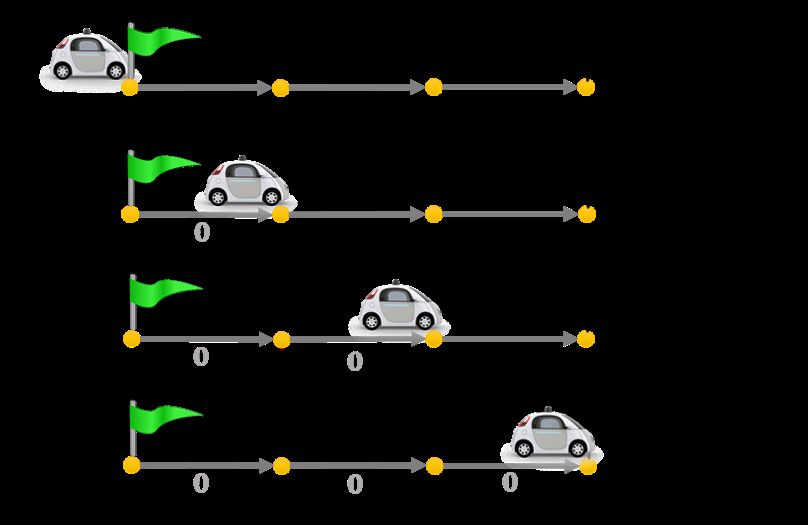
9:2   Traffic Congestion Aware Route Assignment

          A TMS that performs network-level route optimization with CAVs can manage traffic
      congestions effectively as the system can predict the future traffic congestions based on the
      demand and capacity of roads. For example, let us assume that a TMS can predict the
      traffic conditions in the central area of a city as shown in Figure 1, which illustrates the
      general behavior of traffic congestion around the area when the majority of vehicles are
      heading towards the center. Figure 1(a) shows how an increase of traffic demand results
      in the increase of congestion levels. Figure 1(b) shows how a traffic congestion on a grid
      road network propagates to a large area during a certain period of time. Given the traffic
      congestion prediction, the TMS can prevent the predicted traffic congestions by suggesting
      alternative routes to CAVs where possible. In this regard, the TMS has a crucial role in
      shaping the traffic such that vehicles can reach their destinations faster.

          Figure 1 The change of traffic congestion with traffic demand and time: (a) Average waiting
      time per vehicle vs. the number of waiting vehicles [20]; (b) Traffic congestion propagation during a
      period when vehicles are heading toward the center of a city [25, 12]. Road links with darker colour
      have a higher level of congestions.

          The simplest way to assign routes is by utilizing the shortest (fastest) path algorithms [5, 3].
      However, this approach ignores the impact of routes future traffic conditions. Consequently,
      traffic congestions can form on the road segments that are shared by a large number of shortest
      paths. On the other hand, some algorithms assume that a route can affect the travel time of
      other vehicles [11, 15]. This study follows the same assumption. We want to assign routes to
      vehicles effectively to optimize traffic fluency at the network-level. Previously, we proposed
      a centralized routing algorithm for the aforementioned TMS [15]. Our algorithm reduces
      congestion by minimizing intersections between routes. In this work, we propose a route
      assignment algorithm, Traffic Congestion Aware Route Assignment Algorithm (TCARA), to
      mitigate traffic congestions in the central area of a city. To help vehicles avoid future traffic
      congestions, the proposed algorithm uses certain predictive traffic congestion models that
      can estimate the effect of existing routes on the traffic in the future. As traffic optimization
      problems are NP-hard [10] and a TMS needs to respond to navigation requests in a short
      time, our method uses certain traffic heuristics to accelerate the route allocation process.
      We should note that traffic congestion can also happen because of unexpected issues like
      accidents. In such cases, a TMS can resolve the congestion reactively by rerouting vehicles.
      We left such cases for future work. Our algorithm differs from other algorithms substantially
      by proposing a predictive queue-based congestion model. Based on the model and certain
      aggregated traffic information, TCARA optimizes traffic in real time without predicting the
      detailed movement of all individual vehicles, which can result in huge savings in computation
      cost and storage cost. This allows TCARA to assign routes efficiently and enables it to
      outperform state-of-the-art algorithms significantly.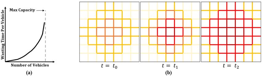
S. Motallebi, H. Xie, E. Tanin, and K. Ramamohanarao                                                   9:3

     The main contributions of our work are summarized as follows.
     We propose a predictive congestion model for route assignment on roads in which the
     dynamic behavior of road links is considered.
     We propose a streaming route assignment algorithm based on the predictive congestion
     model.
     We evaluate our algorithm with a prototype traffic management system based on traffic
     simulation.

    The rest of this paper is organized as follows. Section 2 reviews the related work. Section 3
defines the research problem. Section 4 presents the proposed algorithm. Section 5 reports
experimental results. Section 6 concludes the paper.

 2      Related Work
In this section, we first elaborate on route assignment optimization and the state-of-the-art
algorithms in this area. Then, we review the existing traffic congestion models.

2.1     Route Assignment Approaches
Route assignment optimization is to find the optimal routes for a given set of trip queries.
In this regard, there are two general approaches: user optimum [24] and system optimum [1].
The user-optimum approach, aims to reach an equilibrium state in which no vehicle can find
a faster route than the assigned route. On the other hand, the system-optimum approach
aims to minimize the total travel time for all vehicles. So, in the user-optimum approach,
vehicles with the same source and destination get routes with the same travel time, while
in the system-optimum approach, vehicles with the same source and destination might get
routes with different travel times.
    Route assignment can be static or dynamic. A static traffic assignment is applicable when
the traffic condition is almost stable and route assignment does not lead to the change of
traffic conditions [14]. When traffic condition is not stable, such as when the flow of vehicles
changes quickly like in rush hours, route assignment needs to be dynamic which means the
routes need to be assigned based on the changing traffic conditions [2, 6]. This study is
about a dynamic route assignment algorithm that follows the system-optimum approach.
Existing algorithms in this area are mainly focused on diversifying traffic on alternative
routes to decrease traffic congestion. To achieve this goal, Nguyen et al. [16] propose a
modified version of A* algorithm which suggests alternative routes to vehicles with the same
source and destination. They propose a heuristic function that adds randomness into the
computations of paths. Jeong et al. [11] propose a Self-Adaptive Interactive Navigation Tool
(SAINT) which computes a set of shortest paths for a given source and destination and
selects the path that leads to the minimum increase of congestion level. Vehicles with the
same source and destination are likely to get different routes from SAINT. Zhang et al. [27]
propose an algorithm, DIFTOS, which suggests the shortest path to vehicles initially and
reroutes vehicles based on traffic congestion prediction. As traffic conditions may change
and DIFTOS needs to maintain traffic load for roads at different times, it costs more time
and space compared to other methods. Our previous work addresses a key problem that
causes congestion, which is the intersection of routes at road junctions [15]. We proposed an
algorithm, named MIRA, in which routes are less likely to intersect at junctions compared to
suggesting shortest paths. To assign a route, MIRA divides the road network into blocks and
maintains a heat map showing the average travel times for roads. MIRA also maintains a

                                                                                                    GIScience 2021
9:4 Traffic Congestion Aware Route Assignment
reservation graph showing the impact of allocated routes at each road link on the routes. By
having the data structures, it suggests routes that detour the congested blocks and road links.
We show that the detouring policy leads to a significant reduction of travel time. Among
the described methods, we consider SAINT and MIRA as two baseline methods. It is worth
mentioning that there are iterative dynamic route assignment algorithms [21, 22]. However,
as their time complexity is significantly high, we do not consider them in this study.
2.2 Traffic Congestion Models
Traffic congestion occurs when the traffic load of a road exceeds the available capacity of
the road, leading to the increase of travel time due to the decrease of vehicle speed [13].
According to the literature, congestion on roads leads to the queueing of vehicles. So, the
queue length is a good indicator to quantify congestion levels because a longer queue length
generally indicates a longer travel time on roads [8, 26, 7]. There are also studies that model
traffic congestion based on historical data [12, 25, 4]. However, the historical data might not
always be available. Moreover, such models cannot model traffic congestions that are not
captured well in the historical data. In this study, we use a traffic congestion model based
on queue length.
The queue length is normally measured by the number of vehicles with very low speed on
a road link. It has been used as a measure of congestion named pressure [7]. This simple but
effective measure reveals the congestion level. Pressure-based models are mainly used for
finding the optimal schedule of traffic lights [7, 26, 9]. We utilize this model in our route
assignment algorithms to predict traffic congestion. For a given road network G(V, E), any
edge e ∈ E may have a queue of vehicles waiting at the end vertex (intersection). Whenever
a vehicle stops at an intersection, it adds to the corresponding queue, and after finishing the
edge (i.e., passing the intersection), it leaves the queue. An example scenario with traffic
queues at several intersections is illustrated in Figure 2.
Figure 2 Road network queue model: each edge has a queue containing the vehicles waiting at
its end vertex. More vehicles in a queue indicates higher congestion levels.
It is observed that the congestion level increases linearly with an increase of traffic demand
before the traffic demand reaches a certain threshold, after which the congestion increases
non-linearly. Although the basic version of pressure addresses the linear relationship betweenS. Motallebi, H. Xie, E. Tanin, and K. Ramamohanarao 9:5
traffic load and traffic congestion, it cannot follow the nonlinear behavior of congestion on
the links. Gregoire et al. [7] propose an enhanced version of pressure. The proposed pressure
function (i.e., C(Qe ) defined in Equation 1) models the relationship between the queue length
and the traffic congestion of a road link based on certain key characteristics of road links [7].
Although the pressure function is complex, it has only one variable input, which is the queue
length. In Equation 1, Qe and Ce are the queue length at edge e and the maximum capacity
of edge e, respectively. C∞ and m are two constant parameters. The first parameter, C∞ ,
determines the behavior of edge e for light traffic, and the second parameter, m, is used for
tuning the transition point from linear behavior to nonlinear behavior of edge e. In Section 5,
the model with different values for C∞ and m is analyzed. The model computes the current
congestion value based on the existing vehicles on the roads. The value of the computed
pressure varies between zero (when no vehicle waits on a road, i.e., empty queue) and one
(when the road is full). This pressure can be considered as a real-time congestion model as
it is based on the real-time queue lengths. To model future traffic congestions, the traffic
congestion model needs to be updated such that Qe is based on the number of vehicles that
are going to wait on the roads. To assign routes, we utilize the updated version of this model
in our algorithm (Section 4).
Qe Ce Qe m
C∞ + (2 − C∞ )( Ce )
C(Qe ) = min(1, ) (1)
1+ (Q e m−1
Ce )
3 Problem Definition
I Definition 1 (Delay Function). A delay function (ri , rj ) models the effect of one vehicle
with route rj on a vehicle with route ri .
The delay function gives an extra delay that the vehicle with ri experiences because of
the existence of the vehicle with rj . Apparently, when i = j, the outcome of the epsilon
function is zero as no vehicle has an impact on itself.
I Definition 2 (Delayed Travel Time). A delayed travel time DT T (R0 |R) is the total travel
time of vehicles with all the routes in R0 when there are existing vehicles with all the routes
in R.
Based on the definition, DT T (r|∅) is the shortest possible travel time of a vehicle with
route r, which can be achieved when there is no existing vehicle on the road network.
Equation 2 models travel time of a new vehicle with route r when there are already n vehicles
with assigned routes on the network. The set R contains all the routes of the n existing
vehicles. Each of the existing vehicles can affect the travel time of the new vehicle.
n
X
DT T ({r}|R) = DT T ({r}|∅) + (r|rj ) (2)
j=1
In this study, we assume trip queries arrive at a TMS in a streaming fashion. The
streaming route assignment problem is defined in Equation 3 for a given trip query (i.e., a
pair of source and destination locations).
n
X
r∗ = arg min DT T ({r}|∅) + (r|rj ) (3)
r∈Rcandidate j=1
Problem Statement: Given a trip query from a user and a set of n existing vehicles,
find the optimum route r∗ among the set of candidate routes Rcandidate such that the travel
time of the user is minimized (Equation 3).
GIScience 20219:6 Traffic Congestion Aware Route Assignment
4 Traffic Congestion Aware Route Assignment Algorithm (TCARA)
We propose an algorithm, Traffic Congestion Aware Route Assignment Algorithm (TCARA),
for optimizing route allocation based on the navigation requests from CAVs. TCARA is
based on the A* algorithm that finds route in a weighted graph. The weights are computed
based on the aforementioned congestion model (Section 2.2). As the congestion model uses
the predicted queue length to estimate future congestion levels, it is important to get an
accurate prediction of the queue length. For this purpose, we define Allocated Capacity
(AC) based on the existing routes.
Allocated capacity shows the impact of a vehicle on the queue length at specific road
links. When a vehicle is currently on a road link, we define the allocated capacity of the
vehicle at the edge as 1. When the vehicle leaves the link, the AC of this vehicle at the edge
is 0. The AC values of the vehicle at the links on the remaining of route are higher than
0 but less than 1. The AC values decrease gradually for the links farther away from the
current link of the vehicle, indicating the diminishing impact from the vehicle on the traffic
conditions that are further away into the future. We define AC based on the average travel
times (showing traffic condition of roads) in Equation 4. In the equation, ACei and T Tei
represent the allocated capacity of the ith edge ei in a given route r =< e1 , ..., en > and
the travel time of ei , respectively. Here, n is the number of road links between the vehicle’s
current position and the destination. The travel time at road links is updated frequently by
a TMS. Whenever a vehicle leaves a road link, ACs for the rest of the route are recomputed.
The aggregated value of the ACs at an edge is used as the predicted queue length Qe for
the edge in the congestion model (Section 2.2).By assigning the ACs we would be able to
quantify the influence of all the route allocations on the traffic of a specific edge.
Pi−1
j=1 T Tej
ACei = 1 − Pn (4)
j=1 T T ej
Figure 3 Updating allocated capacity for a given route over time. At t = 5 when the vehicle
leaves e1 , the travel time at e3 increases in 10 min.
Figure 3 shows how AC is computed for a vehicle during its trip. Let us assume a three-
link route is assigned for a given source and destination. As shown in the figure, the AC
0 5 5+10
values at the start of the trip are 1 − 5+10+5 = 1, 1 − 5+10+5 = 0.75, and 1 − 5+10+5 = 0.25S. Motallebi, H. Xie, E. Tanin, and K. Ramamohanarao 9:7
for e1 , e2 , and e3 , respectively. Whenever the vehicle leaves a road segment, the AC values
for the rest of the route are recomputed. Let us assume the travel time of e3 increases to 10
minutes at the 5th minute. The new travel time will be used when updating AC values after
the time point. As the vehicle leaves the first link, ACe1 becomes 0. The second and third
0 10
links get 1 − 10+10 = 1 and 1 − 10+10 = 0.5, respectively. The same procedure runs for the
updates at the 15th minute. At the end of the trip, all AC values become 0.
TCARA needs to maintain the aggregated AC values at road links. The AC values are
used to capture the pressure at the road links based on the congestion model. The traffic
management system (TMS) is responsible for keeping the AC values updated based on the
received location updates from the vehicles. Algorithm 1 defines TCARA with details. This
algorithm is based on the A* algorithm in which the congestion model is utilized as a heuristic
function. TCARA computes the congestion values (pressure values at edges) during its route
search. As vehicles are connected to the TMS, the real-time traffic conditions are available.
For a given pair of source and destination, it computes a route with the minimum value of
congestion. Once a new route is computed by TCARA, the TMS updates aggregated AC
values at the edges on the route. Whenever a vehicle leaves a road link, the aggregated AC
values need to be updated by the TMS as well. Although the route of the vehicle remains
unchanged when the vehicle leaves an edge, the AC values at the edges in the rest of the
vehicle’s path get updated, which can affect the creation of new routes for other vehicles in
the future.
The time complexity of TCARA is the same as Dijkstra’s algorithm, O(|V |log|V | + |E|).
TCARA needs storage in order of O(|V | + |E|) same as Dijkstra’s algorithm. Also, it needs
O(n|E|) for storing the AC values of existing routes (n is the number of vehicles). The cost
of updating the AC values with a route is O(|E|).
5 Experiments
We evaluate the proposed algorithm TCARA. We focus on the traffic scenarios in cities and
assume that there is no street blockage due to accidents or traffic light failures.
5.1 Baseline Approaches
We compare TCARA against several baseline methods, First-In-First-Assigned Fastest (FIFA-
Fastest), SAINT [11], and MIRA [15]. FIFA-Fastest uses Dijkstra’s algorithm to compute
routes with the minimum travel times. Although FIFA-Fastest is a simple algorithm, it is
utilized in well-known navigation tools currently. However, the algorithm does not consider
future traffic conditions as its computation is based on the current travel time at road links.
SAINT is the second traffic assignment baseline method, as described in section 2.1. The third
baseline method is MIRA, as described in section 2.1 as well. MIRA is a state-of-the-art route
assignment algorithm. We also include an algorithm, Time-wise Fastest Route Assignment
(TFRA), as the fourth baseline method. Similar to TCARA, TFRA assigns routes based
on traffic congestion prediction. Both algorithms use the same congestion model as shown
in Equation 1. They differ in the computation of travel cost at the edges. Given a source
and a destination, TFRA searches for a routes based on Dijkstra’s algorithm. When the
search expands to an edge, TFRA estimates the time point at which a vehicle with the new
route arrives at the edge. Then, TFRA estimates the number of existing vehicles that would
be at the edge at that time. The estimated value is used as the queue length (Qe ) in the
congestion model. The pressure value compared with the model is then used as the weight
(travel cost) of the edge.
GIScience 20219:8 Traffic Congestion Aware Route Assignment
Algorithm 1 Traffic Congestion Aware Route Assignment.
Input: Road network graph G(V, E) where any edge em,n has a weight w(em,n ) that equals
to the aggregated AC values at the edge, source s, destination d
Output: Route r from s to d
1: // Vertices in Q are always sorted based on the travel cost between s and the vertices.
2: Q ← Empty-Priority-Queue()
3: for m ∈ V do
4: costm ← ∞; m.previous ← N IL; m.time = 0; Q.insert(m)
5: end for
6: costs ← 0
7: while Q is not empty do
8: m ← vertex in Q with the lowest cost to s
9: remove m from Q
10: if m = d then
11: break;
12: end if
13: for n ∈ End points of the edges starting from m do
14: Cm,n ← C(wm,n ) // Pressure value of em,n based on Equation 1, where the value
of Qe is w(em,n )
15: if costn > costm + Cm,n then
16: costn ← costm + Cm,n
17: n.previous ← m
18: end if
19: end for
20: end while
21: m ← d; L ← Empty-Linked-List() ; L.append(m)
22: while m 6= s do
23: m ← m.previous
24: L.append(m)
25: end while
26: Reverse L // The first item will be source after reverse
27: Return L
5.2 Experiment Environment
We create an experiment environment using a traffic simulator, SMARTS [18], which can
perform real-time microscopic simulation for vehicles on road networks. Kotagiri et al. [18]
show that SMARTS can preform realistic simulations. Moreover, SMARTS simulates adaptive
traffic lights as in the real world, where traffic lights tune their light cycle based on incoming
traffic flows. In our experiments, SMARTS generates trip queries and sends them to a route
allocator, which computes routes and sends them to SMARTS. The routes are assigned to
CAVs in SMARTS. Whenever a CAV leaves a road link, SMARTS gives this information
immediately to the route allocator for updating the weights in TFRA/TCARA. SMARTS
also sends updates of travel time to the route allocator periodically. The travel time of a
road link is the average travel time of CAVs finished the link since the last report. If no CAV
has traveled during a report time interval, we compute the average travel time as the road
link length over the speed limit of the link. The average travel time is used for computing
weights in TFRA/TCARA.S. Motallebi, H. Xie, E. Tanin, and K. Ramamohanarao 9:9
5.3 Performance Metrics
As route assignment algorithms aim to minimize travel time, we define two metrics based
on the travel time of CAVs. The performance metric, Travel Time Ratio at Individual level
(TTRI), measures average travel time for individuals. It is defined in Equation 5, where
T T (vi ), BT T (vi ), and |V| represent the actual travel time of vehicle vi , the best travel time
for vehicle vi , and the number of all vehicles. The actual travel time is the travel time
achieved by following the computed route, while the best travel time is computed based on
the shortest path (in terms of travel time) assuming vehicles always travel at the free flow
speed. We should note that it is not suitable to evaluate the algorithms using the optimum
total travel time, which is the minimum travel time of all trip queries. This is because
obtaining the optimum total travel time implies that trip queries need to be available at first,
while this is not true in the streaming route assignment. Lower TTRI values are better. The
best value is one when the actual travel time of vehicles is equal to their best theoretical
travel times. We also measure gridlock threshold, which is the maximum number of vehicles
that can finish their routes with no gridlock. An increase in traffic load and congestion can
lead to a gridlock where no vehicle can move further. The TTRI metric has no meaningful
values in a gridlock situation. So, all experiment results are limited to gridlock thresholds.
|V|
1 X T T (vi )
T T RI = (5)
|V| i=1 BT T (vi )
5.4 Experimental Settings
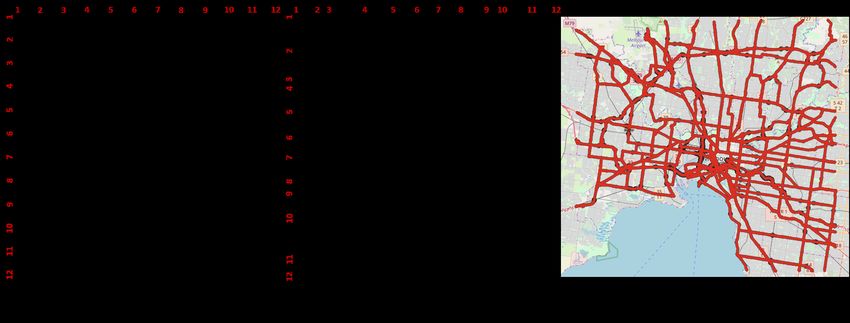
Figure 4 (a) The Manhattan-grid road network used in the experiments where all intersections
are signalized (area statistics 4.4km×4.4km) (b) The semi-real road network used in the experiments
where all intersections are signalized (area statistics 4.4km×4.4km) (c) The real road network
(Metropolitan of Melbourne, Australia) used in the experiments (area statistics 30km×30km) where
most of intersections are signalized.
We investigate the impact of the number of vehicles and the impact of the spatial
distribution of source and destination on all algorithms.
Number of Vehicles is an essential indicator of traffic conditions on the roads. Having
more vehicles on the roads can increase congestion, and its impact can be examined by
measuring travel times. A better algorithm can manage more traffic load with a higher
gridlock threshold. When testing the effect of this parameter, we start from a certain value
and increase the value gradually until all algorithms reach gridlock.
GIScience 20219:10 Traffic Congestion Aware Route Assignment
We consider two distributions for source and destination locations: uniform and Gaussian.
The uniform distribution means the locations are uniformly distributed around the city, while
Gaussian distribution means the locations are more likely to be around the city center. We
define four source-destination distribution scenarios: 1) Uniform-Uniform (representing off-
peak hours), 2) Uniform-Gaussian (representing morning peak hours), 3) Gaussian-Uniform
(representing afternoon peak hours), and 4) Gaussian-Gaussian (representing an extreme case
of congestion at the city center). The default value for this parameter is Gaussian-Gaussian.
We run two experiment sets. In each experiment set, we vary one parameter while keeping
the other parameter at its default value. The first experiment set evaluates the effect of
the number of vehicles, and the second experiment set evaluates the impact of the spatial
distribution of source and destination. Both sets of experiments are conducted with three
road networks as described below.
5.4.1 Manhattan-Grid Road Network
The Manhattan-grid network represents an urban area in which roads are organized as a
grid, which can be seen in some urban areas like Manhattan in New York. It is a 12 by 12
network (Figure 4(a)). All intersections are signalized. A road link between two consecutive
intersections is two-way and 400 meters long. Road links have the same maximum allowable
speed, which is 40 km/h. These settings represent a structured city with the same block
sizes and similar traffic rules. The default number of vehicles is 6000 (as this is the gridlock
threshold for TFRA and SAINT algorithms on this network). The default spatial distribution
is Gaussian-Gaussian.
5.4.2 Semi-real Road Network
We also experiment with a semi-real road network (Figure 4(b)). Compared to the previous
network, the semi-real network has more intersections and road links. All intersections have
traffic lights. This road network represents many real road networks of cities with a dense
central part as a Central Business District area. The maximum speed allowed for each road
link is uniformly random set as 40 km/h or 60km/h. The default value of vehicles is 6000.
The default spatial distribution is Gaussian-Gaussian.
5.4.3 Real Road Network
The real road network covers a 30km × 30km area in Melbourne, shown in Figure 4(c).
The center of the road network is the CBD of Melbourne. The network is extracted from
OpenStreetMap. We preprocessed the map and removed the intermediate nodes that are not
real intersections. The default number of vehicles is 40000. The default spatial distribution
of source and destination is Gaussian-Gaussian.
5.4.4 Parameter Tuning for TFRA and TCARA
The congestion models of TFRA and TCARA are based on the normalized pressure model
expressed in Equation 1. The model has two parameters m and C∞ to fit the behavior of
road links. Figure 5 shows different outputs of the congestion model for four combinations of
m and C∞ . For a road link, when C∞ equals to the capacity of road link, C, the output is a
straight line, shown in green in Figure 5. The bigger value of C∞ results in more bending of
the trend line, shown in blue. The curve needs to be tuned for each road network. We define
the best parameter values for a given road network as the values that lead to the maximumS. Motallebi, H. Xie, E. Tanin, and K. Ramamohanarao 9:11
traffic fluency in terms of TTRI. It is worth mentioning that C∞ ≥ C [7]. The effect of
different m values is shown in the figure in blue and orange lines. Also, the figure depicts the
output curves for two road links with different capacities in blue and red. Gregoire et al. [7]
set m = 4 and C∞ to the largest capacity of road links in the network. As all roads have
almost the same length in the Manhattan-grid network, the model becomes linear which does
not correspond to the non-linear behavior of roads mentioned in Section 4. To get larger
values, we consider C∞ = αCmax . Based on our tests the best parameter values of TFRA
and TCARA for the Manhattan-grid network are m = 4 and α = 11, which result in the
minimum value of TTRI. By doing the same procedure for the semi-real and real networks,
the result shows that m = 4 and α = 1 are the best values. The parameter values are also
suggested in the original study [7].
Figure 5 The capacity aware pressure function with different parameters.
5.5 Results
5.5.1 Manhattan-grid Road Network
Figure 6 TTRI for all algorithms under different traffic loads (number of vehicles) for
(a)Manhattan-grid network, (b)Semi-real network, and (c) real network.
TCARA outperforms all other algorithms except for the light traffic condition, as we
expected in terms of TTRI (Figure 6(a)). As TCARA tries to avoid existing traffic when
computing routes, it suggests longer routes than FIFA-Fastest routes when the traffic load
GIScience 20219:12 Traffic Congestion Aware Route Assignment
is low. However, under normal traffic load, TCARA outperforms other algorithms. The
advantage of TCARA is significant when traffic load is high, which is generally accompanied
by a high level of traffic congestions. As the congestion model helps TCARA to predict
traffic congestion, TCARA can avoid congestion or reduce the propagation of congestion
significantly. We summarize the result of the experiment in terms of the applicability of
algorithms for different traffic loads in Table 1. The table expresses that for light traffic
load, n < 2k, suggesting the fastest routes to vehicles is the best strategy, as there is no
congestion and the impact of routes on each other is negligible. For the low traffic loads,
2k ≤ n < 4k, TCARA outperforms other algorithms slightly. Among the three candidates,
SAINT is the worst choice as it has the biggest time complexity. For the high traffic load,
4k ≤ n < 6k, SAINT cannot avoid gridlocks, and TCARA outperforms MIRA slightly. For
the intensive traffic load, 6k ≤ n ≤ 10k, TCARA is the only algorithm that can manage
traffic effectively. The result shows that TCARA can increase the gridlock threshold by 42%
for the same road network compared with the second-best algorithm MIRA. The baseline
algorithm, TFRA, does not outperform others except FIFA-Fastest. Its gridlock threshold is
the same as SAINT in the Manhattan-grid network.
Table 1 Candidate algorithms for different traffic loads.
# vehicles Candidate Algorithms Description
n < 2k FIFA-Fastest The fastest and most effective
2k ≤ n < 4k TCARA, MIRA, SAINT TCARA performs slightly better
4k ≤ n < 6k TCARA, MIRA TCARA performs slightly better
6k ≤ n ≤ 10k TCARA The only workable algorithm for 7k ≤ n
5.5.2 Semi-real Road Network
The result of the semi-real road network (Figure 6(b)) indicates that TCARA outperforms all
algorithms except for light traffic loads in terms of TTRI. The result shows that FIFA-fastest
is less effective for the same traffic load compared with the previous experiment, but still is
the best solution for light traffic with 1k vehicles. The figure shows that TCARA increases
the gridlock threshold from the second-best approach, MIRA, by 33%. Comparing the result
of the Manhattan-grid and semi-real network, we can see that a more complex road network
topology and a larger variation in speed limits affect the maximum gridlock threshold for
all algorithms significantly. The maximum gridlock threshold decreases by 20% when the
network changes from the Manhattan-grid network to the semi-real network.
5.5.3 Real Road Network
TCARA outperforms all other algorithms under all traffic loads in terms of TTRI for the
real road network (Figure 6(c)). The figure shows that for 10k vehicles TCARA, MIRA,
and SAINT have no significant difference. FIFA-Fastest performs ineffectively and reaches a
gridlock situation at 20k. The other algorithms face gridlock at 40k. TCARA outperforms
MIRA and SAINT by 17% and 32% in terms of TTRI, respectively. By comparing the results
with different maps, we can conclude that the topology of road networks plays a crucial rule
in traffic optimization. Moreover, accurate traffic congestion prediction, as achieved with
TCARA, can help decrease traffic congestion considerably.S. Motallebi, H. Xie, E. Tanin, and K. Ramamohanarao 9:13
5.5.4 Source and Destination Distribution
Figure 7 shows clearly that the distribution of trips affects traffic flow considerably. In the
off-peak (Uniform-Uniform) situation, traffic is distributed uniformly and there is no heavy
congestion. So, the performance of different algorithms is very close to each other. The
figure shows that TCARA is stable for all distributions in all networks. It outperforms all
algorithms in most scenarios as it benefits from a predictive congestion model that helps it to
suggest routes with sufficient detours. Also, TCARA is stable in all situations while others
are sensitive to the road network structure, the traffic distribution, or both. The results show
that the baseline algorithm TFRA works well in off-peak hours. Moreover, by comparing
the results, we can conclude that TFRA works with the real network better than with other
networks. It can be because the travel time estimation becomes more accurate when the
network structure becomes denser at the center. The FIFA-Fastest algorithm faces gridlock
in all scenarios except for the uniform-uniform (off-peak) scenario. From the result, we can
conclude that the algorithms following the system optimum approach (i.e., all algorithms
except FIFA-Fastest) manage traffic significantly better compared with the current navigation
systems that optimize routes independently based on current traffic conditions.
Figure 7 TTRI for different spatial distribution of trips and road networks: (a) Manhattan-grid
network with 6000 vehicles (b) Semi-real network with 6000 vehicles (c) Real network with 40000
vehicles.
5.6 Time Complexity
In this experiment, we compare the computation time of the algorithms based on synthetic
grid networks with 1000 to 10000 vertices. Figure 8 shows that FIFA-Fastest is the fastest
algorithm, and SAINT is the slowest algorithm. Although the time complexity of TFRA,
TCARA, MIRA, and FIFA-Fastest are the same (i.e., O(|V |log|V | + |E|)), FIFA-Fastest runs
faster than others as it has the smallest overhead (i.e., the cost for computing edge weights).
The result shows that TCARA is fast enough for practical use as it can compute a route in
less than 100 milliseconds.
6 Conclusions and Future Work
In this study, we proposed a route assignment algorithm TCARA. We showed that how a
predictive congestion model can help reduce traffic congestion significantly. We evaluated
TCARA under different traffic loads, with various road networks, and different spatial
distribution of source and destination. We showed that TCARA suggests faster routes
compared with the state-of-the-art algorithms. TCARA is tailored for the era of CAVs,
where all the vehicles are coordinated by a central traffic management system. A possible
GIScience 20219:14 Traffic Congestion Aware Route Assignment
Figure 8 Computation time achieved with all algorithms for different road network sizes. The
number of vertices varies from 1000 to 10000.
direction of future work is to incorporate traffic lights directly in our model. In this regard,
considering the light cycles as a parameter to enhance the traffic congestion model and
investigating the models for a road network that has a mix of signalized and unsignalized
intersections are the next steps to extend our algorithm. Another possible direction is
to extend the algorithm for situations when vehicles are not fully autonomous, and the
drivers can decide about their routes which adds unpredictability to the problem. Also, such
real-time network-level traffic optimization can be utilized in the solutions for transport
applications like for transport-as-a-service when there is no personal vehicle and all vehicles
are CAVs. So, a central system navigates all CAVs, while the system receives trip queries in
a streaming fashion.
References
1 Martin Beckmann, Charles B McGuire, and Christopher B Winsten. Studies in the economics
of transportation. https://trid.trb.org/view/91120, 1956.
2 Yi-Chang Chiu, Jon Bottom, Michael Mahut, Alex Paz, Ramachandran Balakrishna, Travis
Waller, and Jim Hicks. Dynamic traffic assignment: A primer. Transportation Research
Circular, 2011.
3 Ugur Demiryurek, Farnoush Banaei-Kashani, and Cyrus Shahabi. A case for time-dependent
shortest path computation in spatial networks. In SIGSPATIAL, pages 474–477. ACM, 2010.
4 Xiaolei Di, Yu Xiao, Chao Zhu, Yang Deng, Qinpei Zhao, and Weixiong Rao. Traffic congestion
prediction by spatiotemporal propagation patterns. In IEEE MDM, pages 298–303, June 2019.
5 Edsger W Dijkstra. A note on two problems in connexion with graphs. Numerische mathematik,
1(1):269–271, 1959.
6 Terry L Friesz and D Bernstein. Analytical dynamic traffic assignment models. In Handbook
of transport modelling, pages 181–195. Elsevier, 2000.
7 Jean Gregoire, Xiangjun Qian, Emilio Frazzoli, Arnaud de La Fortelle, and Tichakorn Wong-
piromsarn. Capacity-aware backpressure traffic signal control. IEEE TCNS, 2(2):164–173,
June 2015.
8 Randolph W Hall. Transportation queueing. In Handbook of Transportation Science, pages
113–153. Springer, 2003.
9 Hsu-Chieh Hu and Stephen F. Smith. Softpressure: A schedule-driven backpressure algorithm
for coping with network congestion. In IJCAI, pages 4324–4330, 2017.S. Motallebi, H. Xie, E. Tanin, and K. Ramamohanarao 9:15
10 Olaf Jahn, Rolf H Möhring, Andreas S Schulz, and Nicolás E Stier-Moses. System-optimal
routing of traffic flows with user constraints in networks with congestion. Operations research,
53(4):600–616, 2005.
11 Jaehoon Jeong, Hohyeon Jeong, Eunseok Lee, Tae Oh, and David Du. SAINT: Self-adaptive in-
teractive navigation tool for cloud-based vehicular traffic optimization. IEEE TVT, 65(6):4053–
4067, 2016.
12 Yuxuan Liang, Zhongyuan Jiang, and Yu Zheng. Inferring traffic cascading patterns. In
SIGSPATIAL, pages 2:1–2:10. ACM, 2017.
13 Tim Lomax, Shawn Turner, Gordon Shunk, Herbert S. Levinson, Richard H. Pratt, Paul N.
Bay, and G. Bruce Douglas. Quantifying Congestion, Volume 1: Final Report. National
Academy Press, Washington, D.C., 1997. URL: https://trid.trb.org/view/475257.
14 Marin Lujak, Stefano Giordani, and Sascha Ossowski. Route guidance: Bridging system and
user optimization in traffic assignment. Neurocomputing, 151:449–460, 2015.
15 Sadegh Motallebi, Hairuo Xie, Egemen Tanin, Jianzhong Qi, and Kotagiri Ramamohanarao.
Streaming route assignment for connected autonomous vehicles (systems paper). In SIGSPA-
TIAL, page 408–411. ACM, 2019.
16 Uyen TV Nguyen, Shanika Karunasekera, Lars Kulik, Egemen Tanin, Rui Zhang, Haolan
Zhang, Hairuo Xie, and Kotagiri Ramamohanarao. A randomized path routing algorithm
for decentralized route allocation in transportation networks. In SIGSPATIAL, pages 15–20.
ACM, 2015.
17 Kotagiri Ramamohanarao, Jianzhong Qi, Egemen Tanin, and Sadegh Motallebi. From how to
where: Traffic optimization in the era of automated vehicles. In SIGSPATIAL, pages 10:1–10:4.
ACM, 2017.
18 Kotagiri Ramamohanarao, Hairuo Xie, Lars Kulik, Shanika Karunasekera, Egemen Tanin,
Rui Zhang, and Eman Bin Khunayn. SMARTS: Scalable microscopic adaptive road traffic
simulator. ACM TIST, 8(2):26:1–26:22, 2016.
19 David Schrank, Bill Eisele, Tim Lomax, and Jim Bak. 2015 urban mobility scorecard. Technical
Report, Texas A&M Transportation Institute, 2015.
20 Cambridge Systematics. Traffic congestion and reliability: Trends and advanced strategies for
congestion mitigation. Technical report, United States. Federal Highway Administration, 2005.
21 WY Szeto and Hong K Lo. Dynamic traffic assignment: properties and extensions. Transport-
metrica, 2(1):31–52, 2006.
22 Nicholas B Taylor. The contram dynamic traffic assignment model. Networks and Spatial
Economics, 3(3):297–322, 2003.
23 Marion Terrill. Stuck in traffic? Road congestion in Sydney and Melbourne, 2017.
https://grattan.edu.au/report/stuck-in-traffic.
24 John Glen Wardrop. Some theoretical aspects of road traffic research. Proceedings of the
Institution of Civil Engineers, 1(3):325–362, 1952.
25 Haoyi Xiong, Amin Vahedian, Xun Zhou, Yanhua Li, and Jun Luo. Predicting traffic congestion
propagation patterns: A propagation graph approach. In IWCTS, pages 60–69. ACM, 2018.
26 Ali A Zaidi, Balázs Kulcsár, and Henk Wymeersch. Back-pressure traffic signal control with
fixed and adaptive routing for urban vehicular networks. IEEE TITS, 17(8):2134–2143, 2016.
27 Weidong Zhang, Nyothiri Aung, Sahraoui Dhelim, and Yibo Ai. DIFTOS: A distributed
infrastructure-free traffic optimization system based on vehicular ad hoc networks for urban
environments. Sensors, 18(8), 2018.
GIScience 2021You can also read