Cryptocurrency Alpha Models via Intraday Technical Trading - Stanford University
←
→
Page content transcription
If your browser does not render page correctly, please read the page content below
Cryptocurrency Alpha Models via Intraday Technical
                    Trading

                                       Amanda Brown
                       Department of Management Science and Engineering
                                      Stanford University
                                      Stanford, CA 94305
                                   amandacb@stanford.edu

                     Jonathan Ling                                      Arjun Sawhney
    Department of Management Science and Engineering             Department of Computer Science
                   Stanford University                                 Stanford University
                   Stanford, CA 94305                                  Stanford, CA 94305
                jonling@stanford.edu                               sawhneya@stanford.edu

                                              Abstract
         Cryptocurrency, a digital currency maintained without a centralized authority, tends
         to be significantly more volatile than stocks, but returns can be significantly greater
         using high-frequency trading strategies. Further, non-technical signals, meaning
         data external to the price and orderbook information such as sentiment analysis
         on social media or Twitter posts, have traditionally been used as key indicators of
         cryptocurrency trends. In contrast, this paper seeks to explore sources of alpha
         or excess returns, that can be found from technical analysis alone, using a pairs
         trading strategy, lagged linear regression and three other machine learning models –
         NeuralProphet, XGBoost and recurrent neural networks. Generally, we found that
         the high volatility of cryptocurrency assets at the hourly level was challenging to
         model but still able to be profitably monetized. The pairs trading approach suffers
         from the fact that few coins are statistically co-integrated, however our lagged
         linear regression model performs best of all of the machine learning models over
         our trading test period with a Sharpe ratio of 3.34.

1   Introduction
Cryptocurrency references digital currency that maintains integrity without being under the control of
a centralized authority. These assets maintain their security because all transactions involving them
are vetted by a blockchain [Royal and Voigt, 2021]. Given their shift in paradigm from traditional
approaches to currency, cryptocurrencies have garnered much interest over the past few years and
this has lead to periods of high growth and fall in their value. They have also been the topic of much
discussion on social media meaning that their value is highly attributed to speculation and there have
been prior works, such as Steinert and Herff [2018], using social network data to forecast their prices.
For our work, we hope to explore sources of alpha (excess returns) in cryptocurrencies that can be
found from technical indicators alone. We focused on predicting our returns on an hourly level, and
describe the specific assets we intended to trade, our data preparation and splitting process in further
detail in the data section. We don’t speculate as to our expected performance on our models given the
high volatility of these assets and periods of high price growth and fall, and instead aim to maximize
our performance on a fixed time period.
As one of the newest financial markets, cryptocurrency has gained much attention in the application
of traditional trading methods such as pairs trading, as well as newer methods in machine learning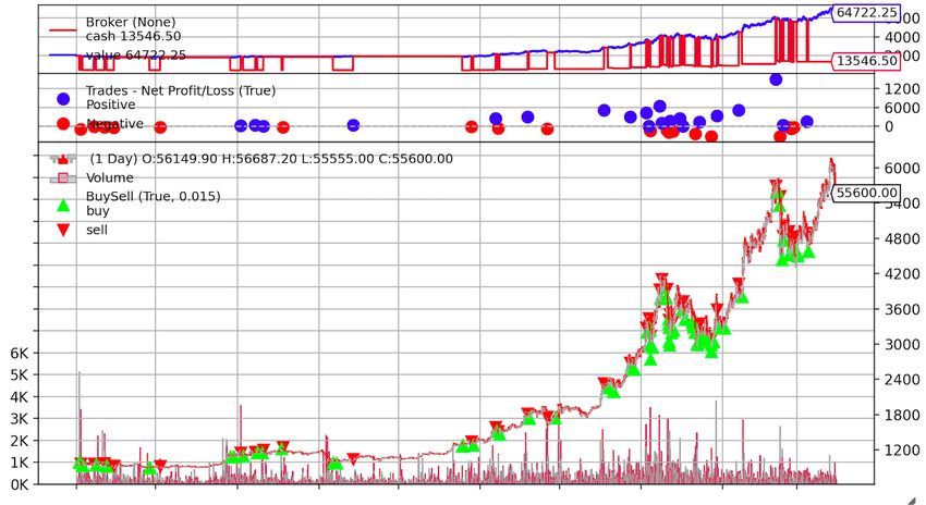
and deep learning. Van den Broek and Sharif [2018] explore cointegration-based pairs trading and
conclude that the Efficient Market Hypothesis does not hold in cryptocurrency markets, meaning that
there is potential to find arbitrage opportunities from all available information. Furthermore, with the
rise of machine learning and deep learning methods, especially related to processing sequence data
such as asset time series, there has been much interest to apply these models to cryptocurrency data,
such as surveyed in Rebane et al. [2018]. In this paper, we explore some of these methods, as well as
other common supervised machine learning predictive methods such as lagged linear regression and
tree boosting. Our main contributions are in providing a method to identify pairs trading windows
and tune model hyperparameters, illustrating methods to increase time series stationarity, extracting
signals from low-volatility predictions, and identifying useful features in lagged linear regression
models for cryptocurrency time series.

2     Data – selection, cleaning and splitting
As of January 2021, there were 7800+ pairs of cryptocurrencies on 500+ cryptocurrency exchanges
and 30+ public APIs available (Wanguba [2021], Zammit [2021], APIs [2021]). We decided use
data from the Bitfinex exchange (from Klein [2021]) as it had significant liquidity, a high degree
of completeness and was convenient to interface with. We also traded the bitcoin-to-US dollar
(BTCUSD) currency pair in our single-pair strategies as it is by far the most commonly traded
pair and thus has the highest liquidity and greatest amount of data available to work with. For our
multiple-pair trading strategies, we used other significantly-traded pairs that we found had the greatest
completeness percentage in the data (BTC, ETH, ZEC, XRP, DOG, DOT, ADA, LTC, XLM).
The raw data from the Bitfinex exchange was at the minute level, but had many data points missing
due to the exchange being closed or down in certain periods, or being open but processing zero
volume. To reduce sensitivity to missing data, we processed it to an hourly level. We did this by
filtering for the on-the-hour timestamps with a ± 2 minute leniency if that particular timestamp was
missing. Specifically, this was done by going through the timestamps at the 58th, 59th, 0th, 1st and
2nd minute closest to the corresponding hour in this order and attributing the first non-missing data
point to that hour.
For the machine learning strategies, we used data from January 1, 2020 to March 31, 2021, at the
hourly level. We then split the data into training, validation and test sets in an 80/10/10 ratio – that is,
the training set being the first 80% of data points in order, the validation set being the next 10% of
data points in order, and the test set being the last 10% of data points in order.

3     Methods
We explored two approaches: a pairs trading strategy and machine learning modeling.

4     Pairs analysis and trading strategy
4.1   Pairs trading method

Pairs trading is a type of statistical arbitrage trading strategy which combines a short position and
a long position in two highly correlated stocks. Given its design, pairs trading is also known as a
market neutral strategy that enables profits in any market conditions. The main steps involved in
implementing a pairs trading strategy are to:

       1. Identify two highly correlated stocks
       2. Enter positions during times of temporarily weaker correlation between the identified stocks
       3. Short an outperforming stock and long an underperforming one
       4. Clear positions when the spread between the stocks converges

To identify the correct pair of stocks, it is common to use a cointegration measure, which is a statistical
test to determine whether two (nonstationary) time series are correlated in the long term (in other
words, whether a linear combination of the two variables is stationary and correlated).

                                                     2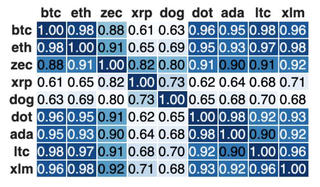
We used a statistical test in the Python package “statsmodels” called “coint” which uses the Engle-
Granger two-step cointegration test, following the method used by Auquan [2017], over the entire
available time horizon for pairs of top-traded assets (fig. 1). The pairs which had a p-value < 0.05
using the cointigration test (allowing us to reject the null hypothesis of “no cointegration”) were
(ETH, XLM), (DOT, ADA) and (LTC, XLM), whose time series are shown in fig. 3.

                               Figure 1: Cointegrated pairs (p < 0.05)

                  (a) XLM vs ETH                                    (b) XLM vs LTC

                                           (c) XRP vs ZEC
                          Figure 2: Cointegrated pairs with p-value < 0.05

We realized that looking over the entire available history to determine cointegration may restrict
our trading ability. We wanted to test a hypothesis that some assets move in and out of windows
of statistically significant cointegration. If this was the case, we could develop a framework for
dynamically checking for cointegration to identify trading opportunities.
The results of this analysis for a trading pair (ZEC/XRP), which performed the best of the numerous
pairs we trialed are in fig. 3a. We selected a look-back window over which to test for cointegration of

                                                  3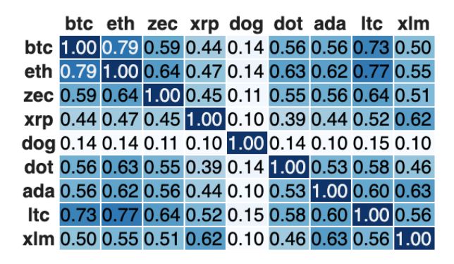
the two time series (5000 hours), repeated the cointegration test every 500 hours, each time marking
statistically significant results which we referred to as “trade” windows (fig. 3b).

   (a) ZEC/XRP cointegration test over look-back         (b) Trade windows determined by p-values < 0.05.
 windows of 5,000 hours, incrementing by 500 hours
                         Figure 3: Cointegration results and trade windows

We found that the regions of cointegration were limited. Unfortunately, when simulating trading on
our test set, the strategy of pairs trading only in “trade” windows yielded significantly worse results.

4.1.1   Z-scoring and rolling averages
With a pairs trading approach, we aim to capitalize on statistical deviations of two stocks, which tend
to move with each other. At a high level, the strategy tracks the ratio of two paired stocks (in our
case, coins), and determines when the short term moving average of the ratio moves out of line (by
±n standard deviations, where n is the threshold selected). This ratio is namely:
                                                         price of asset 1
                             Ratio (asset 1, asset 2) =
                                                         price of asset 2
This requires tracking a short term moving average (we tuned and chose a 12-hour window) and a
long term moving average (similarly, we settled on 480 hours, or 20 days). Figure 4 visualizes these
moving average times series for the ratio of ZEC to XRP.

  Figure 4: Calculating short term and long-term moving averages of the price ratio of ZEC/XRP.

4.1.2   Trading mechanism
Our trading mechanism was to trade whenever the z-score of the moving averages fell outside the
range [-2,2], according to table 1.

                                                     4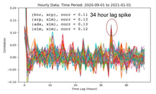
Table 1: Pairs strategy trading mechanism
                When the z-score...                   ...we buy                  ...and we sell
          Exceeds the upper threshold of 2       Ratio* units of asset 2       1 unit of asset 1
        Falls below the lower threshold of -2       1 unit of asset 1       Ratio* units of asset 2
                *“Ratio” is the price ratio between the two assets, i.e., asset 1 / asset 2

Additionally, we cleared positions when the z-score falls between -0.75 and 0.75 and take any profit.
Figure 5 shows the trading signals during all available times and fig. 6 for the trading signals during
only the “trade window” times determined by cointegration tests.

                       Figure 5: Trading signals, using a z-score threshold of 2.

   Figure 6: Trading signals within the “trading windows” only, using a z-score threshold of 2.

4.1.3    Tuning
To tune the strategy for each pair, we computed a Sharpe ratio after simulating trading over the
training window (first 80% of available data). First, we varied the z-score threshold from 1 to 2.5.
For example, for the pair ZEC/XRP, a z-score threshold of 1.75 yielded the highest Sharpe ratio (see
fig. 7a). For the second tuning exercise, the optimal z-score threshold is held constant (1.75), while
the window length of the long-horizon moving average is varied from 1 day (24 hours) to 40 days
(960 hours). For ZEC/XRP, the 408-hour window yielded the best Sharpe ratio of around 1.3 (fig. 7b).
In the test set, the Sharpe ratio was much lower, around 0.11. Returns were also more modest: 1.12%
(not including transaction costs).
Our scheme of identifying cointegrated trading windows doesn’t seem to perform well (we tested
over 25 of the most liquid pairs). Our results with the seemingly best pair (ZEC/XRP) were not

                                                    5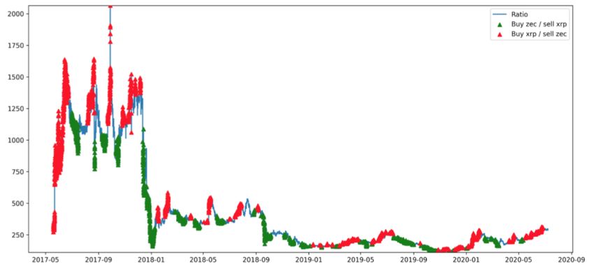
(a) Tuning the z-score threshold, with the optimal       (b) Using the optimal threshold of 1.75, we tuned
                     value being 1.75                          the long-term moving average window length
                                                                      (ranging from 1 day to 40 days)
                              Figure 7: Pairs trading hyperparameter tuning

robust in the testing window (even before trading costs are considered). As a result, we turned to
other models in the next section to try to extract alpha signals.

5     Machine learning models

In our machine learning approach, we used such models to predict a future time series. The machine
models we used were a hand-engineered lagged linear regression model, NeuralProphet (a neural
seasonality and autocorrelation model), XGBoost (an optimized gradient boosting library) and a
recurrent neural network (RNN) with long short-term memory (LSTM) architecture – the last of
which paralleled Saldanha [2020]’s stock trading implementation. We chose these as they are some
of the best and most popular models used for time series prediction. We first pre-processed the data
using methods that befitted the volatile nature of cryptocurrency time series, including testing features
for the lagged linear regression model, and determined how to use the model’s output to make trades.

5.1     Data preparation techniques

One of the biggest challenges in cryptocurrency technical analysis is the high volatility of its time
series and speculative nature of its investors. In this section, we introduce methods to address two
concerns resulting from this volatility – increasing times series stationarity and the relatively lower
volatility of predictions as compared to the actual data.

5.1.1    Increase time series stationarity

It is easier to predict a times series that is stationary, that is, one whose distribution does not change
over time, because less price history and model parameterization is needed to characterize the nature
of the time series in the future. Such a time series when plotted can be recognized by a relatively
constant mean and standard deviation independent of the point in time.
Starting with an asset’s price time series,
                                          the   standard industry practice to increase stationarity is
                                            yt
to convert it into log returns, i.e., log yt−1   , where yt represents the price of the asset at time t.
The log returns time series illustrates volatility clustering, the phenomenon where periods of high
volatility – as indicated by high variance in the series – tend to clump together, and likewise, periods
of low volatility also clump together.
These clumped groups can be thought of as “volatility regimes.” Standardizing the move from one
regime to another can give rise to a further increase in stationarity. We can do this by calculating the
z-score of each data point with respect to a rolling window of say the past 10 points, which produces
a time series that now has significantly more uniform variance.

                                                         6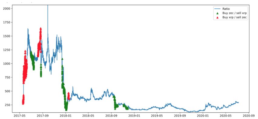
Figure 8: Time series of price, (log) returns and z-scores of (log) returns over time, which illustrates
increasing degrees of stationarity.
5.1.2 Extract signals from low-volatility predictions
We found in modeling time series that the predicted time series had a much lower magnitude and thus
volatility than the actuals time series, as illustrated in fig. 9a.
(a) The predicted time series has a much lower (b) Correlation and hit rate of predicted to actuals
volatility than the actuals time series as seen by its time series by deciles of the predicted values
relatively low magnitudes
Figure 9: Addressing low-volatility predictions (using the XGBoost model results as an example)
To find useful predictive signals in this, we divided the set of predictions into deciles and computed
two metrics by decile:
1. The correlation between the predicted and actual values
2. The “hit rate,” which we define to be the percentage of values in that decile for which the
sign of the predicted and actual values match
An example of the results of this is shown in fig. 9b.
We then used these metrics as signals to trade, and in particular, to use correlation for the magnitude
of the trade and the hit rate for the sign of the trade, if the metric values were far enough away from
their respective baselines to assure confidence in placing those trades.
5.2 Lagged linear regression modeling
5.2.1 Data exploration
During our exploration of the dataset, we calculated the pairwise correlation of the top-traded
cryptocurrency assets. We found high correlation of the returns time series across a handful of assets,
and similar high correlation relationships looking at open price time series between various assets
(fig. 10).
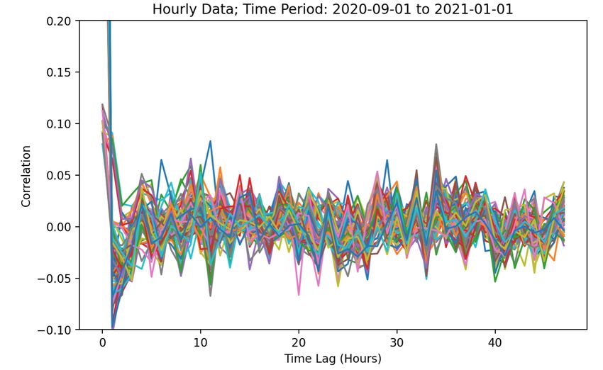
To develop trading insights, we looked into lagged correlations and autocorrelations (in order to find
predictive relationships between the assets). Below is a plot summarizing this analysis. The highest
7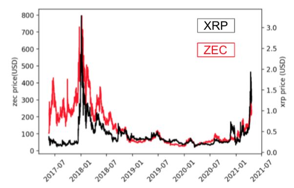
(a) Correlation of returns time series          (b) Correlation of open price time series
                     Figure 10: Correlations between common cryptocurrencies

correlations tended to be the 1 hour lag (of the same asset – for example, BTC vs. BTC lagged by 1
hour). While 1 hour was too short a time horizon to develop a trading strategy over, we looked for
relationships across longer time horizons. We observed a peak at 34-hour lag mark for a handful of
assets (fig. 11), with the top four correlations given in table 2.

Figure 11: Lagged correlation of returns time series for top traded cryptocurrency assets: BTC, ETH,
ZEC, XRP, DOG, DOT, ADA, LTC, XLM.

                          Table 2: Top four correlations at a lag of 34 hours
                          Target asset 34-hour lagged asset Correlation
                              XRP                 XLM                0.13
                              ADA                 XLM                0.13
                              XLM                 XLM                0.12
                              BTC                 XRP                0.11

As such, we began our feature engineering and modeling process by looking into this more closely
and building lagged linear regression models that used 34-hour lagged features for the aforementioned
pairs. The best model of this class of models ended up being the model to predict returns of bitcoin
(BTC) with 34-hour lagged returns of XRP. The results of the model are shown in fig. 13.
The results show that across all deciles, the hit rate was consistently low with respect to the naive
benchmark of 50%. Furthermore, the correlation across all deciles, being less than 0.1, is very low.
These results are not surprising given the volatility of cryptocurrencies, which suggests that there may
be many such fleeting correlations present across shorter time horizons. Furthermore, the features
we used are also highly non-stationary, meaning that it would be exceptionally difficult to predict
cryptocurrency returns on purely lagged features.

                                                   8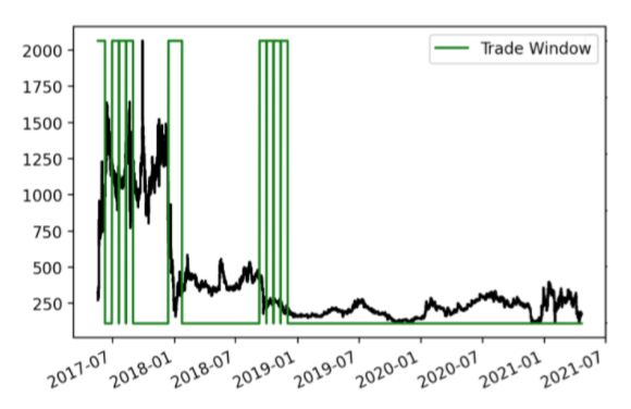
Figure 12: Lagged correlations across coins

                        Figure 13: Predicting BTC with 34-hour lagged XRP

5.2.2   Feature engineering
Given our findings exploring the 34-hour lagged models, we aimed to develop a more unified and
systematic approach to feature engineering. This was particularly important when using linear
regression since carefully crafted features can help to exploit non-linear relationships between the
features and the targets even when this is not a property of the model. We conducted feature
engineering in three categories: time-based features, moving averages and standardization. The
specific classes of features that were tried across each category are shared in table 3 and the final ones
used across each category are in bold in the table.

                               Table 3: Feature engineering attempts
              Feature category                               Approaches tried
   Time-based (across month, day etc) Indicator, integer encoding, trigonometric functions
   Moving averages (across OHLCVT)                 Simple, exponential, weighted
            Standardization                         Z-scoring, min-max scaling
            Bold = features determined as best to use; implemented in final model

Time-based Features
Our intuition behind time based features was that there were likely investors/strategies that would
tend to trade more at specific times of the day or on specific days of the week. These transactions
would affect the volume of cryptocurrency being traded and so affect assets’ proceeding price values
and therefore their returns.
We investigated different variants of time-based features beginning with a simple binary indicator
feature for the hour of day, day of the week and month in the year. This approach, whilst expressive,

                                                    9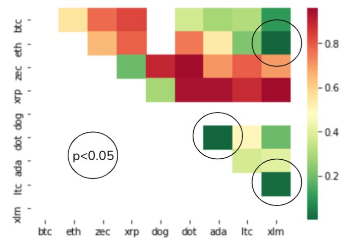
added a significant number of features to our models and so, in order to limit the risk of overfitting,
we also explored integer values for the hours, days and months. While this imposed a relationship
between time-features that may not exist, it reduced the issue of overfitting in practice. We also
recognized that since the time-based features were cyclical, using a purely integer-based approach
(0-11 for months, 0-6 for days) wouldn’t account for the time-continuity of say the months 11 and 0.
As such, we performed trigonometric transformations to account for this but found no significant
benefit over the integer-based approach which we tended to prefer. We also did not use the year as a
feature, since years only roll forward and are not cyclic.
Moving Averages
We found that the non-stationarity of our features made them relatively uninformative when used
alone as regressors in a lagged linear regression model. As such, in order to gain more information
about underlying or longer-term effects affecting the asset pricing, we looked into using moving
averages of our technical features.
As in the pairs trading approach, the idea here is that longer-term moving averages may indicate
a general underlying trend in the asset-pricing that one may be able to exploit, while shorter-term
averages might indicate more recent trends. Oftentimes, as with pairs trading, it is possible to develop
a strategy by comparing both such averages. In particular, there is a theory, as mentioned in Chen
[2021], that short term trends, in asset prices and volatility for example, would, generally, tend to
revert towards their longer term trends.
Given this intuition, we built simple moving averages of features such as open prices, close prices,
volume and number of trades across a range of different time windows and found them to be generally
stronger regressors compared with singular transformations of lagged features. Furthermore, we were
able to glean additional information by calculating not just moving averages, but also the variance of
each statistic over the time window. We also included this for every moving average since this could
help showcase the volatility of the asset and so perhaps help in the prediction process.
We also tried different variants of moving averages with exponential moving averages and weighted
moving averages but we found the additional performance benefit with them to be minimal, par-
ticularly considering the increased amount of complexity and as such, stuck with simple moving
averages.
Standardization
The final category of feature engineering we looked at was standardization. In particular, many
of our initial features were on very different scales and measuring very different things, and so it
would make little sense to add them to the model in their original form, especially with them being
non-stationary.
In order to standardize our features, we mainly focused on using both min-max scaling (subtracting a
feature by it’s minimum value and normalizing by the difference between its maximum and minimum
value) and z-scoring (as described in section 5.1.1). Generally speaking, the performance was quite
similar, however we settled on using z-scoring for all price-based features and features such as volume
and number of trades that weren’t cyclic and used min-max scaling on the time-based features. The
idea here was that for cyclic and integer-based features, the notion of an expected value and standard
deviation would not make much intuitive sense.

5.2.3   General takeaways

When modeling with lagged linear regression, there were a few key findings that affected our final
models and performance.
The use of z-scores on targets was generally effective (particularly over specific time periods) and
so this was an approach we kept consistent over all of our machine learning models. For the lagged
linear regression models, we settled on a z-scoring window of 24 hours, but it’s very possible that
this is a window that could be tuned to be even more effective.
Overfitting tended to be a big problem, namely that strong performance over the training period
wouldn’t continue into the testing period. This was especially prevalent when there were lots of
regressors used in the model. In order to mitigate this, we looked at regularization techniques such as
L1 and L2 regularization, and found that while they reduced the issue, they made it slightly more

                                                  10
difficult to interpret model results intuitively. As such, our approach was to limit the maximum
number of features to be around 15-20 to ensure that our models were small enough to generalize and
allow us to interpret individual feature performance more easily.
We also looked at linear classification models, namely logistic regression models. These tended to
be ineffective when compared with the standard regression models, since the hit rates of both types
of models were similar, while the standard regression models were able to also make predictions of
magnitudes.
5.2.4 Best lagged linear regression model
Our best lagged linear regression model was one that used 5, 10, 15, 20, 50 and 100-hour moving
averages and their variances along with time-based features, in order to predict 24-hour z-scored log
returns.
Our strategy was as follows:
1. Generate feature vector by computing the aforementioned moving averages and variances
and the relevant time-based features
2. Compute predicted (standardized) log-return with model
3. Convert prediction to return space by applying the inverse z-score standardization over the
fixed window and inverse log.
4. If the predicted return was above a (tuned) threshold, buy; if below a (tuned) threshold, sell.
Trade a fixed dollar amount ($1,000 on an initial capital of $20,000)
5. Repeat for next datapoint.
We decided to trade a fixed dollar amount on every trade regardless of the magnitude of the predicted
return, to ensure that our orders would be filled with very high probability.
In order to simulate our model performance, we used Backtrader, a Python backtesting library. The
results of our best lagged regression model are shown in the Results section and also in fig. 14.
5.3 Other machine learning models
We also used NeuralProphet, XGBoost and an RNN LSTM to explore how well these standard
libraries would perform on data processed using our above techniques.
After pre-processing, deciles in the test set were filtered depending on whether the magnitude of
the correlation was above a certain threshold in the validation set. This threshold was tuned as a
hyperparameter to maximize the Sharpe ratio, and the optimal value was selected.
To get the Sharpe ratio, the following trading strategy was used. If the test set decile had a correspond-
ing validation set decile correlation above a given threshold, 0.1 BTC was traded at the next time
point. The magnitude of the trade, 0.1, was chosen to be low enough so as to have a high likelihood
of getting filled, and high enough to be profitable quickly. The sign of the trade was chosen to be
the sign of the validation set’s correlation multiplied by the sign of the validation set’s mean of the
predicted values in their decile. Further, it was observed that the hit rate was typically around the
naive baseline of 0.5, and so it was not used in the trading strategy.
To simulate real trades, as with the lagged linear regression models, we used Backtrader, a backtesting
library.
6 Portfolio construction and risk management approaches
In general, we focused more on the modelling process compared with our portfolio construction and
risk management approaches. However, we did add some intelligence into how we traded and took
positions for some of our models (some of which has been mentioned previously) that we would like
to highlight.
In terms of portfolio construction, given the limited number of cryptocurrency assets with a suffi-
ciently long data history, we considered trading single assets independently. Our focus was also
11predominantly on bitcoin (BTC) as this was the most data-rich coin; and given that we were dealing
with a single asset, we didn’t look into using a portfolio optimizer.
However, within trading in our framework, we added the ability to trade fractions of the asset up to a
specific dollar amount, and also capped each bet at a fixed dollar amount to make sure we didn’t bet
all our capital on a single trade.
We also traded models when their predictions fit into specific deciles in which we had signals
indicating stronger performance, and also looked ahead a several time steps to avoid trading when our
predicted return over a short look-ahead period would cancel out, even when the immediate predicted
return looked promising. This was mainly for models that showed highly variable performance across
deciles in order to improve their performance.
We also looked into adding transaction costs (at 0.3%) in order to evaluate our strategies in a
more realistic setting, an upper bound to Bitfinex’s fees. As expected, the addition of these costs
decreased performance, but since we were unable to assess these transaction costs on our pairs trading
framework, we removed transaction costs from our simulations to maintain a fair comparison.
On the risk management side, we mainly implicitly assessed risk through our use of metrics in
strategy evaluation. The Sharpe ratio normalizes by the variance of the returns and so represents a
metric of risk. We also added stop-loss limits when running our strategy to make sure that if we lost
more than 10% of the initial capital, we would exit our current position and control for big losses.
This was more a threshold/strategy determined a priori and would ideally be something to tune for
the future.
One of the biggest risks with cryptocurrencies in the past, and one that is present in our strategy
when trading big quantities, was the limited liquidity for large positions. This is something that
would have been even more difficult when these assets were less mainstream. However, high returns
on small quantities, and trades across multiple exchanges, would mitigate this risk. Further, this is
becoming less of an issue with these assets appealing more and more to both retail and institutional
investors. There are more exchanges coming up and more market-making firms, and so liquidity is
becoming cheaper and perhaps reducing the risks of developing and executing algorithmic strategies
in cryptocurrencies.
7 Results
The Sharpe ratios from our best-performing models are shown in table 4.
Table 4: Sharpe ratios across models
Model Sharpe ratio
Lagged linear regression 3.34
RNN LSTM 2.64
XGBoost 1.54
ZEC/XRP pairs trading 1.30
NeuralProphet -2.75
Illustrations of model details are shown in figs. 14 to 17 along with simulation performance. Our
strongest model was a lagged linear regression model using moving average and volatility features
with windows of size 5, 10, 20, 50, 100 along with the time-based features mentioned in the feature
engineering section.
12(a) Validation set statistics (b) Backtrader simulation
Figure 14: Lagged linear regression results
(a) Validation set statistics (b) Tuning the threshold hyperparameter
(c) Backtrader simulation with tuned threshold
Figure 15: NeuralProphet results
13(a) Validation set statistics (b) Tuning the threshold hyperparameter
(c) Backtrader simulation with tuned threshold
Figure 16: XGBoost results
(a) Validation set statistics (b) Tuning the threshold hyperparameter
(c) Backtrader simulation with tuned threshold
Figure 17: RNN LSTM results
148 Discussion
Modeling cryptocurrencies with purely technical indicators is a very challenging problem. This is
mainly due to the high volatility shown by these assets and the sudden regime changes from periods
of high growth or high fall due to speculation on a series of platforms. This high volatility makes it
very difficult to find co-integrated assets which could be used in pairs trading strategies and also make
overfitting a big issue in machine-learning models. However, we were able to draw some insights on
how to trade using pairs trading and via machine learning models.
In our view, the pairs trading approach turned out to be a poor strategy for the cryptocurrency universe,
given the paltry number of cointegrated pairs. Perhaps as the space matures, some coins will exhibit
cointegration, but for the time being, the strategy seems inappropriate to be applied for cryptocurrency
pairs, if only using technical indicators.
The lagged linear regression models were generally found to be more robust to the high volatility of
cryptocurrencies. This allowed us to be slightly more simplified (whilst maintaining the strongest
Sharpe ratio) in converting these models into strategies, such as in trading across all deciles. For these
models, we found z-score standardization to be immensely useful for both the targets and features
and found feature engineering with time-based features and moving averages to be more predictive
than just using singular transformations of lagged features.
For the NeuralProphet, XGBoost and RNN models, trading on deciles’ correlations as a signal was
quite effective, even when the correlations were as low in magnitude as 0.05 to 0.2, suggesting that
many relational bets on low correlations can work well. Further, the XGBoost and RNN models
produced positive Sharpe ratios. However, NeuralProphet did not, possibly because its full input,
which was the time series only preceding the first predicted time point, would be stale data when only
using this to predict up to 1.5 months in advance – the duration of each of the validation and test
sets. This could explain why the validation and test set threshold hyperparameter tuning graphs for
NeuralProphet did not show much of a relationship, while those of XGBoost and RNN showed a
stronger relationship, whose input time series ended just before every prediction rather than at the
start of all predictions and so benefited from a more accurate signal.
9 Conclusion
In this paper, we explored how to trade cryptocurrencies at an intraday frequency using technical
analysis only. We found that the high volatility of the time series and low levels of correlation among
liquid cryptocurrency pairs to be the main challenge in profitable trading. In particular, the pairs
trading approach was challenging to monetize as few coins were statistically co-integrated with our
best model having a Sharpe ratio of 1.30. Our machine learning models had varied performance with
Sharpe ratios of -2.75 to 3.34 over the test period, while the best of these being the lagged linear
regression model.
Our main contributions in pairs trading showed how to find cointegrated pairs and tune the ratio time
series z-score threshold and moving average window hyperparameters. In machine learning modeling,
we provided techniques to increase time series stationarity using z-scores, analyze correlation and
hit rate by deciles to extract signals from low-volatility predictions. In particular, we identified that
for our lagged linear regression model, the most useful features for trading were integer encoding
of time-based features, using simple moving averages, and standardization using z-scoring and
min-max-scaling.
10 Future Work
For future work, more generally, we suggest looking into more nuanced techniques in converting our
model to a strategy such as scaling our positions with the magnitude of our predictions in machine
learning models or considered more detailed execution techniques such as shorting and trading on
margin.
We might have also considered pairs analysis of cryptocurrency assets and stocks, to see if other
cointegrated time series exist – for example, with companies that have invested in Bitcoin on their
balance sheet, like Square or Tesla.
15For the NeuralProphet, XGBoost and RNN models, there is also potential to further tune these
models’ hyperparameters and architecture, use more data, incorporate the hit rate information and
use a more sophisticated trading strategy – such as one that varies the magnitude of the trade based
on the magnitude of the correlation.
Given the high volatility and non-stationarity in cryptocurrency time series data, it is important to be
able to model regimes of high growth and high fall well. As such, it would be helpful to complement
technical analysis with news-based and network-based data to infer the sentiment around specific
assets and use them to forecast regime changes. It would also be interesting to look into trading
multiple cryptocurrency assets together or along with other asset types. This would involve delving
further into portfolio optimization and risk management techniques but could be an good way to scale
algorithmic strategies for cryptocurrencies.
References
Public APIs. How many cryptocurrency exchanges are there?, 2021. Public APIs – Cryptocurrency.
Auquan. Pairs trading using data-driven techniques: Simple trading strategies part 3, 12 2017.
https://medium.com/auquan/pairs-trading-data-science-7dbedafcfe5a.
James Chen. Mean reversion, 2 2021. https://www.investopedia.com/terms/m/meanreversion.asp.
Carsten Klein. 400+ crypto currency pairs at 1-minute resolution, 4 2021. https://www.kaggle.com/tencars/392-
crypto-currency-pairs-at-minute-resolution.
Jonathan Rebane, Isak Karlsson, Panagiotis Papapetrou, and Stojan Denic. Seq2seq rnns and arima models for
cryptocurrency prediction: A comparative study. In SIGKDD Fintech’18, London, UK, August 19-23, 2018,
2018.
James Royal and Kevin Voigt. What is cryptocurrency? here’s what you should know, 6 2021.
https://www.nerdwallet.com/article/investing/cryptocurrency-7-things-to-know.
Rodolfo Saldanha. Stock price prediction with pytorch, 6 2020. https://medium.com/swlh/stock-price-prediction-
with-pytorch-37f52ae84632.
Lars Steinert and Christian Herff. Predicting altcoin returns using social media. PloS one, 13(12):e0208119,
2018.
L Van den Broek and Zara Sharif. Cointegration-based pairs trading framework with application to the
cryptocurrency market. Bachelor Thesis, Erasmus University Rotterdam, 2018.
John Wanguba. How many cryptocurrencies are there in 2021?, 1 2021. https://e-cryptonews.com/how-many-
cryptocurrencies-are-there-in-2021/.
Sergio Zammit. How many cryptocurrency exchanges are there?, 4 2021. https://www.cryptimi.com/guides/how-
many-cryptocurrency-exchanges-are-there.
16You can also read


