Pose Machines: Articulated Pose Estimation via Inference Machines
←
→
Page content transcription
If your browser does not render page correctly, please read the page content below
Pose Machines: Articulated Pose Estimation
             via Inference Machines

              Varun Ramakrishna, Daniel Munoz, Martial Hebert,
                    J. Andrew Bagnell, and Yaser Sheikh

                The Robotics Institute, Carnegie Mellon University

      Abstract. State-of-the-art approaches for articulated human pose es-
      timation are rooted in parts-based graphical models. These models are
      often restricted to tree-structured representations and simple parametric
      potentials in order to enable tractable inference. However, these simple
      dependencies fail to capture all the interactions between body parts.
      While models with more complex interactions can be defined, learning
      the parameters of these models remains challenging with intractable or
      approximate inference. In this paper, instead of performing inference on
      a learned graphical model, we build upon the inference machine frame-
      work and present a method for articulated human pose estimation. Our
      approach incorporates rich spatial interactions among multiple parts and
      information across parts of different scales. Additionally, the modular
      framework of our approach enables both ease of implementation with-
      out specialized optimization solvers, and efficient inference. We analyze
      our approach on two challenging datasets with large pose variation and
      outperform the state-of-the-art on these benchmarks.

1   Introduction
There are two primary sources of complexity in estimating the articulated pose
of a human from an image. The first arises from the large number of degrees of
freedom (nearly 20) of the underlying articulated skeleton which leads to a high
dimensional configuration space to search over. The second is due to the large
variation in appearance of people in images. The appearance of each part can
vary with configuration, imaging conditions, and from person to person.
    To deal with this complexity, current approaches [1,2,3,4,5,6] adopt a graph-
ical model to capture the correlations and dependencies between the locations
of the parts. However, inference in graphical models is difficult and inexact in all
but the most simple models, such as a tree-structured or star-structured model.
These simplified models are unable to capture important dependencies between
locations of each of the parts and lead to characteristic errors. One such error—
double counting (see Figure 1)—occurs when the same region of the image is
used to explain more than one part. This error occurs because of the symmet-
ric appearance of body parts (e.g., the left and right arm usually have similar
appearance) and that it is a valid configuration for parts to occlude each other.
Modeling this appearance symmetry and self-occlusion with a graphical model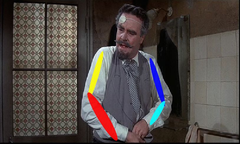
2                                                           Ramakrishna, Munoz, Hebert, Bagnell, Sheikh

                                                        Confidence Maps for Left Leg

                  Pose Inference Machines

                                                                                       Tree Model [5]
                                            Estimated   Stage 1   Stage 2    Stage 3                    Estimated    Max
    Input Image
                                              Pose                                                        Pose      Marginal

Fig. 1: Reducing double counting errors. By modelling richer interactions we pre-
vent the double counting errors that occur in tree models. On the left we show the
belief for the left foot of the person in each stage from our method. The belief quickly
converges to a single sharp peak. On the right, we see that the tree-structured model
[5] has a max-marginal for the left foot with multiple peaks and resulting in both legs
being placed on the same area in the image.

requires additional edges and induces loops in the graph. Such non-tree struc-
tured graphical models typically require the use of approximate inference (e.g.,
loopy belief propagation), which makes parameter learning difficult [7].
     A second limitation of graphical models is that defining the potential func-
tions requires careful consideration when specifying the types of interactions.
This choice is usually dominated by parametric forms such as simple quadratic
models in order to enable tractable inference [1]. Finally, to further enable ef-
ficient inference in practice, many approaches are also restricted to use simple
classifiers such as mixtures of linear models for part detection [5]. These are
choices guided by tractabilty of inference rather than the complexity of the
data. Such trade-offs result in a restrictive model that do not address the inher-
ent complexity of the problem.
     Our approach avoids this complexity vs. tractability trade-off by directly
training the inference procedure. We present a method for articulated human
pose estimation that builds off the hierarchical inference machine originally used
for scene parsing [8,9]. Conceptually, the presented method, which we refer to
as a Pose Machine, is a sequential prediction algorithm that emulates the me-
chanics of message passing to predict a confidence for each variable (part), itera-
tively improving its estimates in each stage. The inference machine architecture
is particularly suited to tackle the main challenges in pose estimation. First,
it incorporates richer interactions among multiple variables at a time, reducing
errors such as double counting, as illustrated in Figure 1. Second, it learns an
expressive spatial model directly from the data without the need for specifying
the parametric form of the potential functions. Third, its modular architecture
allows the use of high capacity predictors which are better suited to deal with
the highly multi-modal appearance of each part. Inspired by recent work [10,11]
that has demonstrated the importance of conditioning finer part detection on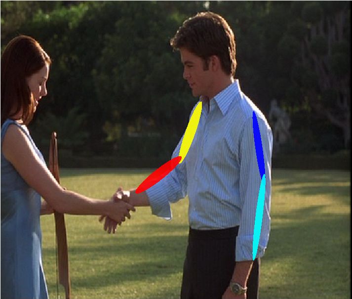
Pose Machines: Articulated Pose Estimation via Inference Machines      3

the detection of larger composite parts in order to improve localization, we in-
corporate these multi-scale cues in our framework by also modeling a hierarchy
of parts.
    Our contributions include a method that simultaneously addresses the two
said primary challenges of articulated pose estimation using the architecture of
an inference machine. Additionally, our approach is simple to implement, requir-
ing no specialized optimization solvers at test time, and is efficient in practice.
Our analysis on two challenging datasets demonstrates that our approach im-
proves upon the state-of-the-art and offers an effective, alternative framework to
address the articulated human pose estimation problem.

2   Related Work

There is a vast body of work on the estimation of articulated human pose from
images and video. We focus on methods to estimate the 2D pose from a single
image. The most popular approach to pose estimation from images has been
the use of pictorial structures. Pictorial structure models [1,2,3,4,5,6], express
the human body as a tree-structured graphical model with kinematic priors that
couple connected limbs. These methods have been successful on images where
all the limbs of the person are visible, but are prone to characteristic errors such
as double-counting image evidence, which occur because of correlations between
variables that are not modeled by a tree-structured model.
    Pictorial structure models with non-tree interactions have been employed
[12,13,14,15] to estimate pose in a single image. These models augment the
tree-structure to capture occlusion relationships between parts not linked in
the tree. Performing exact inference on these models is typically intractable and
approximate methods at learning and test time need to be used. Recent methods
have also explored using part hierarchies [16,17] and condition the detection of
smaller parts that model regions around anatomical joints on the localization
of larger composite parts or poselets [11,10,18,19] that model limbs in canonical
configurations and tend to be easier to detect.
    The above models usually involve some degree of careful modeling. For ex-
ample, [3] models deformation priors by assuming a parametric form for the
pairwise potentials, and [5] restricts the appearance of each part to belong to a
mixture model. These trade-offs are usually required to enable tractable learn-
ing and inference. Even so, learning the parameters of these models usually
involves fine-tuned solvers or approximate piecewise methods. Our method does
not require a tailor-made solver, as its modular architecture allows us to leverage
well-studied algorithms for the training of supervised classifiers.
    In [20], the authors use a strong appearance model, by training rotation
dependent part detectors with separate part detectors for the head and torso
while using a simple tree-structured model. In [21] better part detectors are
learned by using multiple stages of random forests. However this approach uses
a tree-structured graphical model to enforce spatial consistency. Our approach
generalizes the notion of using the output of a previous stage to improve part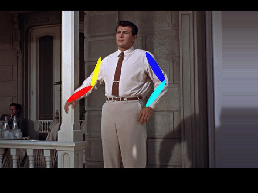
4                                 Ramakrishna, Munoz, Hebert, Bagnell, Sheikh

localization, learns a spatial model in a non-parametric data-driven fashion and
does not require the design of part-specific classifiers.
    Our method bears some similarity to deep learning methods [22] in a broad
sense of also being a multi-layered modular network. However, in contrast to
deep-learning methods which are trained in a global fashion (e.g., using back-
propagation), each module is trained locally in a supervised manner.
    Our method reduces part localization to a sequence of predictions. The use of
sequential predictions—feeding the output of predictors from a previous stage to
the next—has been revisited in the literature from time to time. Methods such as
[23,24] applied sequential prediction to natural language processing tasks. While
[25] explored the use of context from neighboring pixel classifiers for computer
vision tasks. Our approach is based on the hierarchical inference machine ar-
chitecture [8,9] that reduces structured prediction tasks to a sequence of simple
machine learning subproblems. Inference machines have been previously studied
in image and point cloud labeling applications [8,26]. In this work, our contri-
bution is to extend and analyze the inference machine framework for the task of
articulated pose estimation.

3     Pose Inference Machines
3.1     Background
We view the articulated pose estimation problem as a structured prediction
problem. That is, we model the pixel location of each anatomical landmark
(which we refer to as a part) in the image, Yp ∈ Z ⊂ R2 , where Z is the
set of all (u, v) locations in an image. Our goal is to predict the structured
output Y = (Y1 , . . . , YP ) for all P parts. An inference machine consists of a
sequence of multi-class classifiers, gt (·), that are trained to predict the location
of each part. In each stage t ∈ {1 . . . T }, the classifier predicts a confidence for
assigning a location to each part Yp = z, ∀z ∈ Z, based on features of the image
data xz ∈ Rd and contextual information from the preceeding classifier in the
neighborhood around each Yp . In each stage, the computed confidences provide
an increasingly refined estimate for the variable. For each stage t of the sequence,
the confidence for the assignment Yp = z is computed and denoted by
                                                P
                                                              !
                                       p
                                               M
                                                          i
                       bt (Yp = z) = gt xz ;       ψ(z, bt−1 ) ,                   (1)
                                             i=1

where

                            bpt−1 = {bt−1 (Yp = z)}z∈Z ,                          (2)
is the set of confidences from the previous classifier evaluated at every location z
for the p’th part. The feature function ψ : Z × R|Z| → RL   dc
                                                               computes contextual
features from the classifiers’ previous confidences, and       denotes an operator
for vector concatenation.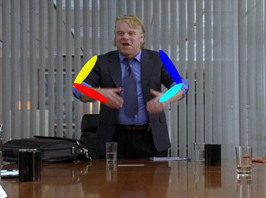
Pose Machines: Articulated Pose Estimation via Inference Machines                                         5

                                                           1                                       1
                                                               xz                                      xz

                                                 Level 1
                                                                             1
                                                                                 b1   (z, 1 b1 )                     1
                                                                                                                         b2
 Image Location z                     l 1 9
                                       bt >                         1
                                                                        g1                                  1
                                                                                                                g2
                                           >
                                           >
                                           >
                                           >
                                           >
                                           >
                                      l 2 >
                                           >               2
                                                               xz                                  2
                                                                                                       xz
                                       bt >>
                                           >
                                           >                                          (z, 2 b1 )

                                                 Level 2
                1
                    xz                     >
                                           >                                 2
                                                                                 b1                                  2
                                                                                                                         b2
                                           >
                                           =
                         l                                          2                                       2
                             gt                                         g1                                      g2
                                       bt l bt
                                      l 3
                                           >
                                           >
                                           >
                                           >
                                           >
                                           >
                                                           L
                                                               xz                                  L
                                                                                                       xz
                                           >
                                           >

                                                 Level L
                                           >
                                           >                                          (z, 3 b1 )
                                           >
                                           >                                 L
                                                                                 b1                                  L
                                                                                                                         b2
                                           >
                                           >                        L                                       L
                                           >
                                           >                            g1                                      g2
                                           ;
 Input Image                          l Pl
                                       bt
                                                               Stage t = 1                             Stage t = 2            Stage t = T
               (a)                                                                         (b)

Fig. 2: (a) Multi-class prediction. A single multiclass predictor is trained for each
level of the hierarchy to predict each image patch into one of Pl + 1 classes. By evalu-
ating each patch in the image, we create a set of confidence maps l bt . (b) Two stages
of a pose inference machine. In each stage, a predictor is trained to predict the
confidence of the output variables. The figure depicts the message passing in an infer-
ence machine at test time. In the first stage, the predictors produce an estimate for
the confidence of each part location based on features computed on the image patch.
Predictors in subsequent stages, refine these confidences using additional information
from the outputs of the previous stage via the context feature function ψ.

   Unlike traditional graphical models, such as pictorial structures, the inference
machine framework does not need explicit modeling of the dependencies between
variables via potential functions. Instead, the dependencies are arbitrarily com-
bined using the classifier, which potentially enables complex interactions among
the variables. Directly training the inference procedure via a sequence of simpler
subproblems, allows us to use any supervised learning algorithm to solve each
subproblem. We are able to leverage the state-of-the-art in supervised learning
and use a sophisticated predictor capable of handling multi-modal variation. As
detailed in the following section, our approach to articulated pose estimation
takes the form of a hierarchical mean-field inference machine [8], where the con-
textual information that each variable uses comes from neighboring variables in
both scale and space in the image.

3.2     Incorporating a Hierarchy

Recent work [11,10] has shown that part detections conditioned on the location
of larger composite parts improves pose estimation performance; however, these
composite parts are often constructed to form tree graph structures [16]. In-
spired by these recent advances, we design a hierarchical inference machine that
similarly encodes these interactions among parts at different scales in the image.
We define a hierarchy of parts from smaller atomic parts to larger composite
parts. Each of the L levels of the hierarchy have parts of a different type. At the
coarsest level, the hierarchy is comprised of a single part that captures the whole
body. The next level of the hierarchy is comprised of composite parts that model
full limbs, while the finest level of the hierarchy is comprised of small parts that
model a region around an anatomical landmark. We denote by P1 , . . . , PL , the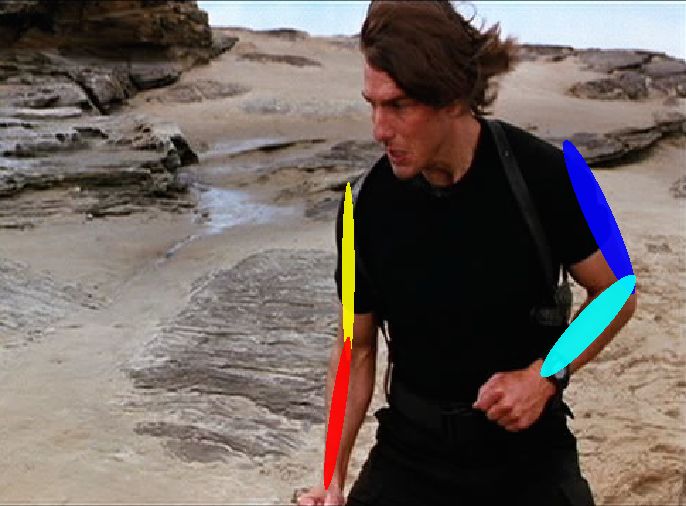
6                                     Ramakrishna, Munoz, Hebert, Bagnell, Sheikh

number of parts in each of the L levels of the hierarchy. In the following, we
denote l gtp (·) as the classifier in the tth stage and lth level that predicts the score
for the pth part. While separate predictors could be trained for each part p in
each level l of the hierarchy, in practice, we use a single multi-class predictor
that produces a set of confidences for all the parts from a given feature vector
at a particular level in the hierarchy. For simplicity, we drop the superscript and
denote this multi-class classifier as l gt (·).
    To obtain an initial estimate of the confidences for the location of each part,
in the first stage (t = 1) of the sequence, a predictor l g1 (·) takes as input features
computed on a patch extracted at an image location z, and classifies the patch
into one of Pl part classes or a background class (see Figure 2a), for the parts
in the lth level of the hierarchy. We denote by xlz , the feature vector of an image
patch for the lth level of the hierarchy centered at location z in the image. A
classifier for the lth level of the hierarchy in the first stage t = 1, therefore
produces the following confidence values:
                                            l
                          l
                              g1 (xlz ) →        bp1 (Yp = z)   p∈0...Pl
                                                                           ,         (3)

where l bp1 (Yp = z) is the score predicted by the classifier l g1 for assigning the
pth part in the lth level of the hierarchy in the first stage at image location z.
Analogous to Equation 2, we represent all the confidences of part p of level l
evaluated at every location z = (u, v)T in the image as l bpt ∈ Rw×h , where w
and h are the width and height of the image, respectively. That is,
                               l p
                                bt [u, v]   = l bpt (Yp = (u, v)T ).                 (4)

For convenience, we denote the collection of confidence maps for all the parts
belonging to level l as l bt ∈ Rw×h×Pl (see Figure 2a).
    In subsequent stages, the confidence for each variable is computed similarly
to Equation 1. In the order to leverage the context across scales/levels in the
hierarchy, the prediction is defined as
                                           !
                         M
              l
                gt xlz ,      ψ(z, l bt−1 ) → l bpt (Yp = z) p∈0...P .       (5)
                                                                               l
                        l∈1...L

As shown in Figure 2b, in the second stage, the classifier l g2 takes as input the
features xlz and features computed on the confidences via the feature function ψ
for each of the parts in the previous stage. Note that the the predictions for a part
use features computed on outputs of all parts and in all levels of the hierarchy
({l bt−1 }l∈1...L ). The inference machine architecture allows learning potentially
complex interactions among the variables, by simply supplying features on the
outputs of the previous stage (as opposed to specifying potential functions in
a graphical model) and allowing the classifier to freely combine contextual in-
formation by picking the most predictive features. The use of outputs from all
neighboring variables, resembles the message passing mechanics in variational
mean field inference [9].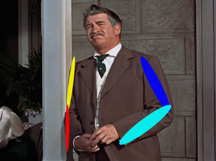
Pose Machines: Articulated Pose Estimation via Inference Machines      7

                                 z            l 1                    l 2   l 3   l Pl
                                               bt                     bt    bt    bt

                                              c1 (z, l b1t )

                                 bt )
                                 l
                          (a)

                                 1 (z,
                                 bt )
                                         c2 (z, l b1t )
                           (b)

                                 l
                                 2 (z,
                                                          l 1
                                         l 1               oK
                                          o1
                                                     l 1
      Input Image                                     o2

Fig. 3: Context Feature Maps (a) Context patch features are computed from each
score map for each location. The figure illustrates a 5 × 5 sized context patch (b) The
context offset feature comprises of offsets to a sorted list of peaks in each score map.

3.3 Context Features
To capture the spatial correlations between the confidences of each part with re-
spect to its neighbors, we describe two types of factors with associated “context”
feature maps denoted by ψ1 and ψ2 .
Context Patch Features. The feature map ψ1 at a location z takes as input
the confidence maps for the location of each part in a hierarchy level l and
produces a feature that is a vectorized patch of a predefined width extracted at
the location z in the confidence map l bpt (see Figure 3a). We denote the set of
patches extracted and vectorized at the location z, from the beliefs of the parts
in the hierarchy level l, by c1 (z, l bpt−1 ). The feature map ψ1 is therefore given
by:                                          M
                       ψ1 (z, l bt−1 ) =          c1 (z, l bpt−1 ).              (6)
                                                          p∈0...Pl

In words, the context feature is a concatenation of scores at location z extracted
from the confidence maps of all the parts in each level the hierarchy. The context
patch encodes neighboring information around location z as would be passed as
messages in a factor graph. Note that because we encode the context from all
parts, this would be analogous to having a graphical model with a complete
graph structure and would be intractable to optimize.
Context Offset Features. We compute a second type of feature, ψ2 , in order
to encode long-range interactions among the parts that may be at non-uniform,
relative offsets. First, we perform non-maxima suppresion to obtain a sorted list
of K peaks from each of the Pl confidence maps l bpt−1 for all the parts in the l’th
hierarchy level. Then, we compute the offset vector in polar coordinates from
location z to each k th peak in the confidence map of the pth part and lth level
denoted as as l opk ∈ R+ × R (see Figure 3b). The set of context offset features
computed from one part’s confidence map is defined as:

                            c2 (z, l bpt−1 ) = l op1 ; . . . ; l opK .           (7)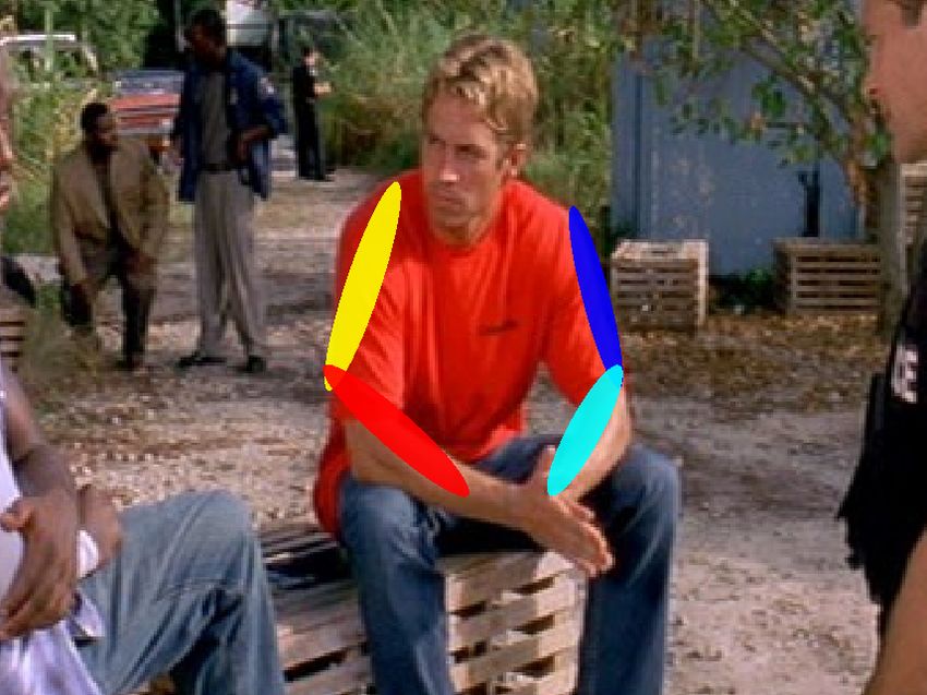
8                                    Ramakrishna, Munoz, Hebert, Bagnell, Sheikh

Algorithm 1 train pose machine
 1: Initialize: l b0 = ∅ l∈1,...,L


 2: for t = 1 . . . T do
 3:    for i = 1 . . . N do
 4:       Create {l bt−1 }L                                       l
                           l=1 for each image i using predictor gt−1 using Eqn. 5.
 5:       Append features extracted from each training image i, and from corresponding
          {l bt−1 }Ll=1 (Eqns. 6 & 8), to training dataset Dt , for each image i.
 6:    end for
 7:    Train l gt using Dt .
 8: end for
 9: Return: Learned predictors {l gt }.

Then, the context offset feature map ψ2 is formed by concatenating the context
offset features c2 (z, l bpt−1 ) for each part in the the hierarchy:
                                              M
                            ψ2 (z, l bt−1 ) =       c2 (z,l bpt−1 ).       (8)
                                            p∈1...Pl

    The context patch features (ψ1 ) capture coarse information regarding the
confidence of the neighboring parts while the offset features (ψ2 ) capture pre-
cise relative location information. The final context feature ψ is computed by
concatenating two: ψ(·) = [ψ1 (·) ; ψ2 (·)].

3.4    Training

Training the inference procedure involves directly training each of the predictors,
{l gt }, in each level l ∈ {1, . . . , L}, and for each stage t ∈ {1, . . . , T }. We describe
our training procedure in Algorithm 1. Training proceeds in a stage-wise man-
ner. The first set of predictors {l g1 } are trained using a dataset D0 consisting
of image features on patches extracted from the training set of images at the
annotated landmarks. For deeper stages, the dataset Dt is created by extracting
and concatenating the context features from the confidence maps {l bt−1 }L             l=1 for
each image, at the annotated locations.

3.5    Stacking

Training the predictors of such an inference procedure is prone to overfitting.
Using the same training data to train the predictors in subsequent stages will
cause them to rely on overly optimistic context from the previous stage, or
overfit to idiosyncrasies of that particular dataset. Ideally we would like to train
the subsequent stages with the output of the previous stages similar to that
encountered at test time. In order to achieve this, we use the idea of stacked
training [27,23].
    Stacked training aims to prevent predictors trained on the output of the first
stage from being trained on same training data. Stacking proceeds similarly to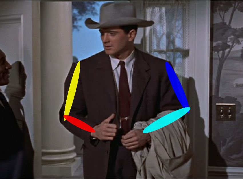
Pose Machines: Articulated Pose Estimation via Inference Machines                     9

                                                Hierarchy Level 1                    Hierarchy Level 2
                                      Head    L.Knee      R.Knee    L.Ank   R.Ank   L.Leg       R.Leg

                           Stage 1
                           Stage 2
                           Stage 3

      Input Image

Fig. 4: The output of a three stage pose inference machine at each stage.
An inference machine iteratively produces more refined estimates of the confidence for
the location of each part. In the first stage, the estimate produced only from image
features is noisy and has multiple modes. Subsequent stages refine the confidence based
on predictions from neighboring factors to a sharp unimodal response at the correct
location and suppress false positive responses in the background. The confidences from
left to right are for the head, left-knee, right-knee, left-ankle, right-ankle, left-leg, right-
leg.

cross-validation by making M splits of the training data D into training and
held-out data {Dm , D/Dm }m=1...M . For each predictor we aim to train in the
first stage, we make M copies, each trained on one of the M splits of the training
data. To create the training data for the next stage, for each training sample, we
use the copy of the predictor that has not seen the sample (i.e., the sample is in
the held-out data for that predictor). Proceeding in this way creates a dataset
to train the next stage on the outputs of the previous stage, ensuring that the
outputs mimic test-time behavior. We repeat the stacking procedure for each
subsequent stage. The stacking procedure is only performed during training to
create a training dataset for subsequent stages. At test time, we use a predictor
in each stage that is trained using all of the data.

3.6    Inference
At test time, inference proceeds in a sequential fashion as show in Figure 2b.
Features are extracted from patches of different scales (corresponding to each
of the L levels of the hierarchy) at each location in the image and input to the
first stage classifiers {l g1 }L                                               l   L
                               l=1 , resulting in the output confidence maps { b1 }l=1 .
Messages are passed to the classifiers in the next stage, by computing context
features via the feature maps ψ1 , ψ2 on the confidences l b1 from the previous
stage. Updated confidences {l b2 }L                                        l
                                        l=1 are computed by the classifiers g2 and this
procedure is repeated for each stage. The computed confidences are increasingly
refined estimates for the location of the part as shown in Figure 4. The location
of each part is then computed as,
                                     ∀l, ∀p, l yp∗ = argmax l bpT (z).                              (9)
                                                          z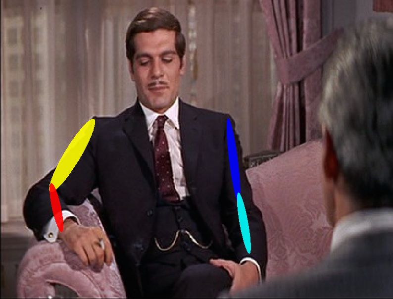
10                              Ramakrishna, Munoz, Hebert, Bagnell, Sheikh

The final pose is computed by directly picking the maxima of the confidence
map of each part after the final stage.

3.7   Implementation

Choice of Predictor. The modular nature of the inference machine architecture
allows us to insert any supervised learning classifier as our choice of multi-class
predictor g. As the data distribution is highly multi-modal, a high-capacity non-
linear predictor is required. In this work, we use a boosted classifier [28] with
random forests for the weak learners, because random forests have been empir-
ically shown to consistently outperform other methods on several datasets [29].
We learn our boosted classifier by optimizing the non-smooth hinge loss [30].
We use 25 iterations of boosting, with a random forest classifier. Each random
forest classifier consists of 10 trees, with a maximum depth of 15 and with a split
performed only if a node contained greater than 10 training samples.
Training. To create positive samples for training, we extract patches around the
annotated anatomical landmarks in each training sample. For the background
class, we use patches sampled from a negative training corpus as in [5]. In addi-
tion, in subsequent stages, we sample negative patches from false positive regions
in the positive images.
Image Features. We extract a set of image features from a patch at each
location in the image. We use a standard set of simple features to provide a
direct comparison and to control for the effect of features on performance. We
use Histogram of Gradients (HOG) features, Lab color features, and gradient
magnitude. The HOG features are defined based on the structure of the human
poses labeled in the respective datasets, which we detail in the follow section.
In the FLIC dataset [11], only an upper-body model is annotated and we use 6
orientations with a bin size 4. In the LEEDS dataset [6], a full body model is
annotated and we use 6 orientations with a bin size of 8 in the finest level of the
hierarchy. We increase the bin size by a factor of two for the coarser levels in
the hierarchy. For the upper body model, we model each part in the finest level
of the hierarchy with 9 × 9 HOG cells, while we use 5 × 5 HOG cells for the full
body model. These parameter choices are guided by previous work using these
datasets [11,5].
Context Features. For the context patch features, we use a context patch of
size 21 × 21, with max-pooling in each 2 × 2 neighborhood resulting in a set of
121 numbers per confidence map. For the context offset features we use K = 3
peaks.

4     Evaluation

We evaluate and compare the performance of our approach on two standard pose
estimation datasets to the current state-of-the-art methods.
Pose Machines: Articulated Pose Estimation via Inference Machines                                                                                              11

                   Method               Torso Upper Lower Upper Lower Head Total
                                               Legs  Legs Arms Arms
                   Ours                 93.1  83.6  76.8  68.1   42.2 85.4 72.0
                   Pishchulin [20]       88.7  78.8  73.4  61.5 44.9 85.6 69.2
                   Pishchulin [10]       87.5  75.7  68.0  54.2  33.8 78.1 62.9
                   Yang&Ramanan [5] 84.1       69.5  65.6  52.5  35.9 77.1 60.8
                   Eichner&Ferrari [31] 86.2   74.3  69.3  56.5  37.4 80.1 64.3

Table 1: Quantitative performance on LEEDS Sports Pose dataset. Perfor-
mance is measured by the PCP metric on the test set of the LEEDS sports dataset.
Our algorithm outperforms all current methods.

                      FLIC: Localization Accuracy              Effect of number of stages of sequence (T)on performance (FLIC)                  Effect of number of stages of sequence (T)on performance (FLIC)
                                                                              100                                                                              100
           100                                                                           Elbow Acc - 1 Stage
                    MODEC [Sapp 13] elbow acc                                                                                                                          Wrist Acc - 1 Stage
                                                                               90        Elbow Acc - 2 Stages                                                   90     Wrist Acc - 2 Stages
                    MODEC [Sapp 13] wrist acc                                            Elbow Acc - 3 Stages                                                          Wrist Acc - 3 Stages
            80      poseMachines (Ours) elbow acc                              80                                                                               80
                    poseMachines (Ours) wrist acc
                                                                               70                                                                               70
Accuracy

                                                                                                                                                    Accuracy
                                                                   Accuracy

            60                                                                 60                                                                               60
                                                                               50                                                                               50
            40                                                                 40                                                                               40
                                                                               30                                                                               30
            20                                                                 20                                                                               20
                                                                               10                                                                               10

                        5            10             15    20                        2      4     6     8        10   12   14   16   18   20                                5                  10   15         20
                 Normalized Distance Threshold (pixels)                                 Normalized Distance Threshold (pixels)                                       Normalized Distance Threshold (pixels)
                                       (a)                                                                                                    (b)

Fig. 5: (a) Comparison to state-of-the-art on FLIC Elbow and wrist localization
accuracy on the FLIC dataset. We achieve higher accuracies for both joints compared
to the state-of-the-art [11]. (b) Effect of number of stages. We plot the change
in accuracy with the number of stages in the sequence. We observe that including a
second stage which uses contextual information greatly increases the performance. We
also observe a slight improvement with the incorporation of an additional third stage.

LEEDS Sports Pose Dataset. We evaluate our approach on the LEEDS
sports dataset [6] which consists of 1,000 images for training and 1,000 images
for testing. The images are of people in various sport poses. We use the observer-
centric annotations as used in [10] for training and testing. We train a full body
model comprised of a 2-level hierarchy. The second level of the hierarchy com-
prises of the 14 parts corresponding to each of the annotated joints. The first level
comprises of 6 composite parts formed by grouping parts belonging to each of
the limbs, a composite part for the head and shoulders and a composite part for
the torso. Parameter choices were guided by a grid search using a development
subset of the training dataset comprising of 200 images. We use the Percentage
Correct Parts (PCP) metric to evaluate and compare our performance on the
dataset. The results are listed in the Table 1. We outperform existing methods
and achieve an average PCP score of 72.0. We show qualitative results of our
algorithm on a few representative samples from the LEEDS dataset in Figure 7.
FLIC Upper Body Pose Dataset. We also evaluate our approach on the FLIC
dataset [11] which consists of still frames from movies. The dataset consists of
4,000 images for training and 1,000 images for testing. We use a model trained
to recognize the pose of the upper body. We employ a two-level hierarchy, with
12 Ramakrishna, Munoz, Hebert, Bagnell, Sheikh
Elbow Wrists Knee Ankle
1 1 1 1
Elbow- st1 Wrists- st1 Knee- st1 Ankle- st1
Elbow- st2 Wrists- st2 Knee- st2 Ankle- st2
0.8 Elbow- st3 0.8 Wrists- st3 0.8 Knee- st3 0.8 Ankle- st3
0.6 0.6 0.6 0.6
Accuracy
Accuracy
Accuracy
Accuracy
0.4 0.4 0.4 0.4
0.2 0.2 0.2 0.2
0 0 0 0
0 0.1 0.2 0.3 0.4 0 0.1 0.2 0.3 0.4 0 0.1 0.2 0.3 0.4 0 0.1 0.2 0.3 0.4
Normalized dist. thresh. (pixels) Normalized dist. thresh. (pixels) Normalized dist. thresh. (pixels) Normalized dist. thresh. (pixels)
Fig. 6: Effect of number of stages on LSP. We plot the change in accuracy with
the number of stages in the sequence for difficult landmarks on the LEEDS Sports
dataset. The additional stages improve the performance especially of difficult parts
like the elbows and wrists.
the finest level of the hierarchy comprising of seven parts corresponding to the
annotated anatomical landmark locations, the second level comprising of three
composite parts corresponding to each of the arms and one for the head and
shoulders. Parameter choices were guided by a grid search using a development
subset of the training dataset comprising of 200 images. We use the accuracy
metric specified in [11]. In Figure 5a we plot the accuracy of the wrist and elbow
joints. Our approach shows a significant improvement over the state of the art
[11]. We show qualitative results of our algorithm on samples from the FLIC
dataset in Figure 8.
Effect of the number of stages. We study the effect of increasing the num-
ber of stages T in the inference machine. Figure 5b plots the part localization
accuracy as a function of the distance from the ground truth label on the FLIC
dataset. We see that predicting part location only based on image features (T =
1) results in poor performance. The addition of a second stage (T = 2) that in-
corporates contextual information results in a dramatic increase in the accuracy.
An additional third stage (T = 3) adds a minor increase in performance on this
dataset. Setting the number of stages is similar to how the number of iterations
are set for message-passing algorithms such as belief propagation. For datasets
of different sizes the number of stages can be set by evaluating the change in
loss after each iteration.
We plot the change in accuracy with the number of stages in the sequence for
difficult landmarks on the LEEDS Sports dataset (see Figure 6). We observe that
including a second stage which uses contextual information greatly increases the
performance. We also observe slight improvements for the knees and ankles, and
a significant improvement for the wrists and elbows upon adding a third stage.
5 Discussion
We have presented an inference machine for articulated human pose estimation.
The inference machine architecture allows us to learn a rich spatial model and
incorporate high-capacity supervised predictors, resulting in substantially im-
proved pose estimation performance. One of the main challenges that remainPose Machines: Articulated Pose Estimation via Inference Machines 13
Fig. 7: Qualitative example results on the LEEDS sports dataset. Our algo-
rithm is able to automatically learn a spatial model and correctly localize traditionally
difficult parts such as the elbows and wrists.
is to correctly handle occluded poses, which is one of the failure modes of the
algorithm (see Figure 9). A second failure mode is due to rare poses for which
there are too few similar training instances. Tackling these challenges will need
an understanding of the requirements from a human pose dataset for training
an algorithm to work in the wild. The ability to handle complex variable depen-
dencies leads to interesting directions for future work that include extending the
method to monocular video by incorporating temporal cues, directly predict-
ing poses in 3D, and adapting the method for different categories of articulated
objects.
Acknowledgements: This material is based upon work supported by the Na-
tional Science Foundation under Grants No. 1353120 and 1029679 and the NSF
NRI Purposeful Prediction project.
References
1. Felzenszwalb, P.F., Huttenlocher, D.P.: Pictorial structures for object recognition.
IJCV (2005)
2. Ramanan, D., Forsyth, D.A., Zisserman, A.: Strike a Pose: Tracking people by
finding stylized poses. In: CVPR. (2005)
3. Andriluka, M., Roth, S., Schiele, B.: Monocular 3D Pose Estimation and Tracking
by Detection. In: CVPR. (2010)
4. Andriluka, M., Roth, S., Schiele, B.: Pictorial Structures Revisited: People Detec-
tion and Articulated Pose Estimation. In: CVPR. (2009)
5. Yang, Y., Ramanan, D.: Articulated pose estimation with flexible mixtures-of-
parts. In: CVPR. (2011)14 Ramakrishna, Munoz, Hebert, Bagnell, Sheikh
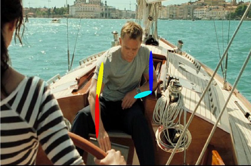
Fig. 8: Qualitative example results on the FLIC dataset. Our algorithm is able
to automatically learn a spatial model and correctly localize traditionally difficult parts
such as the elbows and wrists.
Fig. 9: Failure Modes. Typical failure modes include severe occlusion of parts and
rare poses, for which too few training samples exist in the training set. The method is
also prone to error when there are multiple people in close proximity.
6. Johnson, S., Everingham, M.: Clustered pose and nonlinear appearance models for
human pose estimation. In: BMVC. (2010)
7. Kulesza, A., Pereira, F.: Structured learning with approximate inference. In: NIPS.
(2007)
8. Munoz, D., Bagnell, J.A., Hebert, M.: Stacked hierarchical labeling. In: ECCV.
(2010)
9. Ross, S., Munoz, D., Hebert, M., Bagnell, J.A.: Learning message-passing inference
machines for structured prediction. In: CVPR. (2011)Pose Machines: Articulated Pose Estimation via Inference Machines 15
10. Pishchulin, L., Andriluka, M., Gehler, P., Schiele, B.: Poselet conditioned pictorial
structures. In: CVPR. (2013)
11. Sapp, B., Taskar, B.: MODEC: Multimodal Decomposable Models for Human Pose
Estimation. In: CVPR. (2013)
12. Wang, Y., Mori, G.: Multiple tree models for occlusion and spatial constraints in
human pose estimation. In: ECCV. (2008)
13. Sigal, L., Black, M.J.: Measure locally, reason globally: Occlusion-sensitive articu-
lated pose estimation. In: CVPR. (2006)
14. Lan, X., Huttenlocher, D.P.: Beyond trees: Common-factor models for 2d human
pose recovery. In: ICCV. (2005)
15. Karlinsky, L., Ullman, S.: Using linking features in learning non-parametric part
models. In: ECCV. (2012)
16. Tian, Y., Zitnick, C.L., Narasimhan, S.G.: Exploring the spatial hierarchy of mix-
ture models for human pose estimation. In: ECCV. Springer (2012)
17. Sun, M., Savarese, S.: Articulated part-based model for joint object detection and
pose estimation. In: ICCV. (2011)
18. Gkioxari, G., Arbeláez, P., Bourdev, L., Malik, J.: Articulated pose estimation
using discriminative armlet classifiers. In: CVPR, IEEE (2013)
19. Wang, Y., Tran, D., Liao, Z.: Learning hierarchical poselets for human parsing.
In: CVPR, IEEE (2011)
20. Pishchulin, L., Andriluka, M., Gehler, P., Schiele, B.: Strong appearance and
expressive spatial models for human pose estimation. In: ICCV. (2013)
21. Dantone, M., Gall, J., Leistner, C., Van Gool, L.: Human pose estimation using
body parts dependent joint regressors. In: CVPR. (2013)
22. Bengio, Y.: Learning deep architectures for AI. Foundations and trends in Machine
Learning (2009)
23. Carvalho, V., Cohen, W.: Stacked sequential learning. In: IJCAI. (2005)
24. Daumé III, H., Langford, J., Marcu, D.: Search-based structured prediction. Ma-
chine Learning (2009)
25. Bai, X., Tu, Z.: Auto-context and its application to high-level vision tasks and 3d
brain image segmentation. PAMI (2009)
26. Xiong, X., Munoz, D., Bagnell, J.A., Hebert, M.: 3-d scene analysis via sequenced
predictions over points and regions. In: ICRA. (2011)
27. Wolpert, D.H.: Stacked Generalization. Neural Networks (1992)
28. Friedman, J.H.: Greedy function approximation: a gradient boosting machine.
Annals of Statistics (2001)
29. Caruana, R., Niculescu-Mizil, A.: An empirical comparison of supervised learning
algorithms. In: ICML. (2006)
30. Grubb, A., Bagnell, J.A.: Generalized boosting algorithms for convex optimization.
In: ICML. (2011)
31. Eichner, M., Ferrari, V.: Appearance sharing for collective human pose estimation.
In: ACCV. (2012)You can also read