Continual Reinforcement Learning with Multi-Timescale Replay
←
→
Page content transcription
If your browser does not render page correctly, please read the page content below
Continual Reinforcement Learning with
                                                                 Multi-Timescale Replay

                                                                                  Christos Kaplanis
                                                                               Department of Computing
                                                                               Imperial College London
arXiv:2004.07530v1 [cs.LG] 16 Apr 2020

                                                                        christos.kaplanis14@imperial.ac.uk

                                                             Claudia Clopath ∗                           Murray Shanahan *
                                                        Department of Bioengineering                   Department of Computing
                                                          Imperial College London                      Imperial College London /
                                                        c.clopath@imperial.ac.uk                              DeepMind
                                                                                                     m.shanahan@imperial.ac.uk

                                                                                          Abstract

                                                      In this paper, we propose a multi-timescale replay (MTR) buffer for improving
                                                      continual learning in RL agents faced with environments that are changing con-
                                                      tinuously over time at timescales that are unknown to the agent. The basic MTR
                                                      buffer comprises a cascade of sub-buffers that accumulate experiences at different
                                                      timescales, enabling the agent to improve the trade-off between adaptation to new
                                                      data and retention of old knowledge. We also combine the MTR framework with
                                                      invariant risk minimization [Arjovsky et al., 2019] with the idea of encouraging the
                                                      agent to learn a policy that is robust across the various environments it encounters
                                                      over time. The MTR methods are evaluated in three different continual learning
                                                      settings on two continuous control tasks and, in many cases, show improvement
                                                      over the baselines.

                                         1       Introduction

                                         Artificially intelligent agents that are deployed in the real world have to be able to learn from data
                                         streaming in from a nonstationary distribution and incrementally build on their knowledge over time,
                                         while operating with limited computational resources; this is the challenge of continual learning
                                         [Ring, 1994]. Artificial neural networks (ANNs), however, have long been known to suffer from the
                                         problem of catastrophic forgetting [McCloskey and Cohen, 1989], whereby, in a context where the
                                         data distribution is changing over time, training on new data can result in abrupt erasure of previously
                                         acquired knowledge. This precludes them from being able to learn continually.
                                         Typically, the testing of methods for mitigating catastrophic forgetting has been conducted in the
                                         context of training on a number of distinct tasks in sequence. A consequence of this format for
                                         evaluation is that many continual learning techniques make use of the boundaries between tasks
                                         in order to consolidate knowledge during training [Ruvolo and Eaton, 2013, Kirkpatrick et al.,
                                         2017, Zenke et al., 2017]. In the real world, however, changes to the data distribution may happen
                                         gradually and at unpredictable timescales, in which case many of the existing techniques are simply
                                         not applicable, prompting the community to pose task-agnostic and task-free continual learning as
                                         desiderata for our agents [clw, 2016, 2018].
                                             ∗
                                                 Equal Contribution.

                                         Preprint. Under review.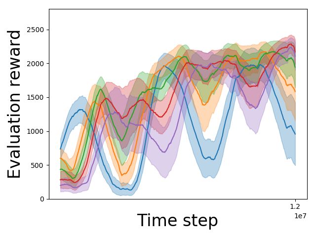
Reinforcement learning [Sutton and Barto, 1998] is a paradigm that naturally poses these challenges,
where the changes to the data distribution can occur unpredictably during the training of a single
task and can arise from multiple sources, e.g.: (i) correlations between successive states of the
environment, (ii) changes to the agent’s policy as it learns, and (iii) changes to the dynamics of
the agent’s environment. For these reasons, catastrophic forgetting can be an issue in the context
in deep reinforcement learning, where the agents are neural network-based. One commonly used
method to tackle (i) is experience replay (ER) [Lin, 1992, Mnih et al., 2015], whereby the agent’s
most recent experiences are stored in a first-in-first-out (FIFO) buffer, which is then sampled from at
random during training. By shuffling the experiences in the buffer, the data are then identically and
independently distributed (i.i.d.) at training time, which prevents forgetting over the (short) timescale
of the buffer since the distribution over this period is now stationary.

1.1   Experience replay for continual reinforcement learning

The community has naturally investigated whether ER can be used to mitigate forgetting over the
longer timescales that are typically associated with continual learning, particularly because it does
not necessarily require prior knowledge of the changes to the data distribution. One key observation
that has been made in both a sequential multi-task setting [Isele and Cosgun, 2018, Rolnick et al.,
2019], as well as in a single task setting [de Bruin et al., 2015, 2016, Zhang and Sutton, 2017,
Wang and Ross, 2019], is that it is important to maintain a balance between the storage of new and
old experiences in the buffer. By focusing just on recent experiences, the agent can easily forget
what to do when it revisits states it has not seen in a while, resulting in catastrophic forgetting and
instability; by retaining too many old experiences, on the other hand, the agent might focus too much
on replaying states that are not relevant to its current policy, resulting in a sluggish and/or noisy
improvement in its performance.
In this paper, we propose a multi-timescale replay (MTR) buffer to improve continual reinforce-
ment learning, which consists of a cascade of interacting sub-buffers, each of which accumulates
experiences at a different timescale. It was designed with the following three motivating factors:

      • Several of the previously mentioned replay methods use just two timescales of memory in
        order to strike a balance between new and old experiences [Isele and Cosgun, 2018, Rolnick
        et al., 2019, Zhang and Sutton, 2017]. For example, one method in [Isele and Cosgun, 2018]
        combines a small FIFO buffer with a reservoir buffer that maintains a uniform distribution
        over the agent’s entire history of experiences [Vitter, 1985] - this means that the composition
        of the replay database will adjust to short term changes in the distribution (with the FIFO
        buffer) and to long term changes (with the reservoir buffer), but it will not be as sensitive to
        medium term changes. Our method, on the other hand, maintains several sub-buffers that
        store experiences at a range of timescales, meaning that it can adjust well in scenarios where
        the rate of change of the distribution is unknown and can vary over time.
      • The MTR buffer also draws inspiration from psychological evidence that the function
        relating the strength of a memory to its age follows a power law [Wixted and Ebbesen,
        1991]; forgetting tends to be fast soon after the memory is acquired, and then it proceeds
        slowly with a long tail. In the MTR buffer, as a result of the combination of multiple
        timescales of memory, the probability of a given experience lasting beyond a time t in the
        database also follows a power law; in particular, it approximates a 1t decay (Appendix A.3).
      • While shuffling the data to make it i.i.d. helps to prevent forgetting, it also discards structural
        information that may exist in the sequential progression of the data distribution - something
        that it is preserved to a degree in the cascade of sub-buffers in the MTR method. Invariant
        risk minimization (IRM) is a recently developed method that uses the assumption that the
        training data has been split up into different environments in order to train a model that is
        invariant across these environments and is thus more likely to be robust and generalise well.
        In a second version of the MTR model, the MTR-IRM agent, we apply the IRM principle
        by treating each sub-buffer as a different environment to see if it can improve continual
        learning by encouraging the agent to learn a policy that is invariant over time.

We test the two MTR methods in RL agents trained on continuous control tasks in a standard RL
setting, as well as in settings where the environment dynamics are continuously modified over time.
We find that the standard MTR agent is the best continual learner overall when compared to a

                                                    2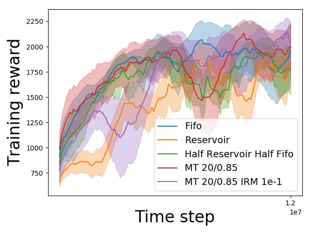
number of baselines, and that the MTR-IRM agent improves continual learning in some of the more
nonstationary settings, where one would expect an invariant policy to be more beneficial.

2     Preliminaries
2.1   Soft Actor-Critic

We used the soft actor-critic (SAC) algorithm [Haarnoja et al., 2018a] for all experiments in this
paper, adapting the version provided in [Hill et al., 2018]. SAC is an actor-critic RL algorithm based
on the maximum entropy RL framework, which generalises the standard RL objective of maximising
return by simultaneously maximising the entropy of the agent’s policy:
                                          "∞                                  #
                                           X
                         ∗                        t
                       π = arg max Eπ           γ (r(st , at ) + αH(π(·|st )))                     (1)
                                     π
                                              t=0

where st and at represent the state visited and action taken at time t respectively, r(st , at ) is the
reward at time t, π is a stochastic policy defined as a probability distribution over actions given state,
π ∗ represents the optimal policy, γ is the discount factor, H is the entropy and α controls the balance
between reward and entropy maximisation. This objective encourages the agent to find multiple ways
of achieving its goal, resulting in more robust solutions. Robustness was a particularly important
factor in choosing an RL algorithm for this project, since the added nonstationarity of the environment
in two of the experimental settings can easily destabilise the agent’s performance easily. In initial
experiments, we found that SAC was more stable that other algorithms such as DDPG [Lillicrap
et al., 2015]. We used the automatic entropy regulariser used in [Haarnoja et al., 2018b], which was
found to be more robust than a fixed entropy regularisation coefficient.

2.2   Invariant Risk Minimisation

Invariant risk minimisation [Arjovsky et al., 2019] is an approach that seeks to improve out-of-
distribution generalisation in machine learning models by training them to learn invariant or stable
predictors that avoid spurious correlations in the training data, a common problem with the framework
of empirical risk minimisation [Vapnik, 2006]. While typically the training data and test data are
randomly shuffled in order to ensure they are from the same distribution, IRM poses that information
is actually lost this way, and it starts with the assumption that the data can be split up into a number
of different environments e ∈ Etr . The IRM loss function encourages the model to learn a mapping
that is invariant across all the different training environments, with the hope that, if it is stable across
these, then it is more likely to perform well in previously unseen environments. The IRM loss is
constructed as follows:
                                     X
                             min          Re (Φ) + λ · ||∇w|w=1.0 Re (w · Φ)||2                          (2)
                          Φ:X →Y
                                   e∈Etr

where Φ is the mapping induced by the model that maps the inputs to the outputs (and is a function
of the model parameters), Re is the loss function for environment e, w is a dummy variable and λ is
a parameter that balances the importance of the empirical loss (the first term) and the IRM loss (the
second term). The goal of the IRM loss is to find a representation Φ such that the optimal readout
w is the same (i.e. the gradient of the readout is zero), no matter the environment; this way, when
a new environment is encountered, it is less likely that the policy will have to change in order to
suit it. In the next section, we describe how the IRM principle is applied in one version of the MTR
replay database where the different environments correspond to experiences collected at different
timescales.

3     Multi-Timescale Replay
The multi-timescale replay (MTR) database of size N consists of a cascade of nb FIFO buffers, each
with maximum size nNb , and a separate overflow buffer (also FIFO), which has a dynamic maximum
size that is equal to the difference between N and the number of experiences currently stored in
the cascade (Figure 1(a)). New experiences of the form (st , at , rt+1 , st+1 ) are pushed into the first
sub-buffer. When a given sub-buffer is full, the oldest experience in the buffer is pushed out, at which

                                                     3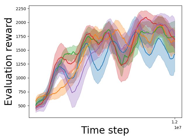
point it has two possible fates: (i) with a predefined probability βmtr it gets pushed into the next
sub-buffer, or (ii) with probability 1 − βmtr it gets added to the overflow buffer. If the total number
of experiences stored in the cascade and the overflow buffer exceeds N , the overflow buffer is shrunk
with the oldest experiences being removed until the database has at most N experiences. Once the
cascade of sub-buffers is full, the size of the overflow buffer will be zero and any experience that is
pushed out of any of the sub-buffers is discarded. During training, the number of experiences sampled
from each sub-buffer (including the overflow buffer) is proportional to the fraction of the total number
of experiences in the database contained in the sub-buffer. Figure 1(b) shows the distribution of ages
of experiences in the MTR buffer, and a mathematical intuition for how the MTR buffer results in a
power law distribution of memories is given in Appendix A.3.

                               (a)                                                 (b)
Figure 1: (a) Diagram of MTR buffer; each blue box corresponds to a FIFO sub-buffer. (b) Histogram
of age of experiences in cascade of MTR buffer after 5 million experiences inserted.

3.1       IRM version of MTR

In the IRM version of the MTR agent (MTR-IRM), we assume that the set of experiences in each
sub-buffer of the MTR cascade corresponds to data collected in a different environment. Under this
assumption, we can apply the IRM principle to the policy network of the SAC agent, so each Re (Φ)
corresponds to the policy loss calculated using the data in the corresponding sub-buffer. While it
would be interesting to apply the IRM to the value losses too, in this work, for simplicity we only
applied it to the policy loss of the agent. The per-experience policy loss for SAC is as follows:
                           Lπ (φ, s) = Ea∼πφ [αt log(πφ (a|s)) − Qθ1 (s, a)]                          (3)
where φ are the parameters of the policy network, πφ is the conditional action distribution implied
by the policy network, s is the state, a is the action sampled from πφ , αt is the dynamic entropy
coefficient and Qθ1 is the Q-value function implied by one of the two Q-value networks used in SAC.
The policy loss at each iteration is calculated by averaging the per-experience loss shown above over
a mini-batch of experiences chosen from the replay database. In combination with IRM, however, the
overall policy loss is as evaluated as follows:
                                               nb
                                             X       |Di |
                                                              Est0 ∼Di ||∇w|w=1.0 Lπ (φ, st0 , w)||2 (4)

 LπIRM (φ) = Est ∼D [Lπ (φ, st )]+λIRM ·
                                              i=1
                                                  |Dcascade |
where |Di | is the number of experiences in the ith sub-buffer in the cascade, |Dcascade | is the total
number of experiences stored in the cascade of sub-buffers, w is a dummy variable, and Lπ is
overloaded, such that:
                     Lπ (φ, st0 , w) = Ea∼πφ [αt log(πφ (w · a|s)) − Qθ1 (s, a)]                    (5)
The balance between the original policy loss and the extra IRM constraint is controlled by λIRM .

4         Experiments
4.1       Setup

The two MTR methods were evaluated in RL agents trained with SAC [Haarnoja et al., 2018a] on two
different continuous control tasks (RoboschoolAnt and RoboschoolHalfCheetah)2 , where the strength
      2
    These environments are originally from [Schulman et al., 2017] and were modified by adapting code from
[Packer et al., 2018].

                                                    4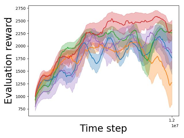
of gravity in the environments was modified continuously throughout training in three different ways:
fixed gravity, linearly increasing gravity, and gravity fluctuating in a sine wave. The idea was to see
how the agents could cope with changes to the distribution that arise from different sources and at
different timescales. In the fixed gravity setting, which constitutes the standard RL setup, the changes
to the distribution result from correlation between successive states and changes to the agent’s policy.
In the other two settings, continual learning is made more challenging because changes are also made
to the dynamics of the environment. In the linear setting, the gravity is adjusted slowly over time,
with no setting being repeated at any point during training; in the fluctuating setting, the changes are
faster and gravity settings are revisited so that the relearning ability of the agent can be observed.
In order to evaluate the continual learning ability of the agents, their performance was recorded over
the course of training (in terms of mean reward) on (i) the current task at hand, and (ii) on an evenly
spaced subset of the gravity environments experienced during training (−7, −9.5, −12, −14.5 and
−17m/s2 ). It is worth noting that initial experiments were run in a traditional multi-task setting,
where the gravity was uniformly sampled from an interval of [−17, −7] throughout training, i.e. the
tasks are interleaved, in order to ensure that it is possible to learn good policies for all tasks in the
same policy network (Figure A.2). Further experimental details and a table of the hyperparameters
used for training are given in Appendix A.4.

4.2   Results

Across all three continual learning settings, the basic MTR agent appears to be the most consistent
performer, demonstrating either the best or second best results in terms of training reward and mean
evaluation reward in all tasks, indicating that recording experiences over multiple timescales can
improve the tradeoff between new learning and retention of old knowledge in RL agents. The
MTR-IRM agent achieved the best evaluation reward in two of the more nonstationary settings for
the HalfCheetah task, but not in the Ant task, indicating that learning a policy that is invariant across
time can be beneficial for generalisation and mitigating forgetting, but that it might depend on the
particular task setting and the transfer potential between the different environments. Below, we
discuss the results from each setting in more detail. All plots show moving averages of mean reward
over three runs per agent type with standard error bars.

Fixed gravity In the fixed gravity experiments, the FIFO and MTR agents were consistently the
best performers (Figure 2), with both agents achieving a similar final level of training reward in both
the HalfCheetah and Ant tasks. One would expect the FIFO agent to be a relatively strong performer
in this setting, since the environment dynamics are stable and so the retention of old memories is
likely to be less crucial than in the other two more nonstationary settings. The fact that the basic
MTR agent performs as well as the FIFO agent shows that the replay of some older experiences is not
holding back the progress of the agent, but also that it does not seem to particularly help the overall
performance either. The MTR-IRM agent, on the other hand, performed poorly in the fixed gravity
setting, presumably because there is not enough nonstationarity to reap any generalisation benefits
from learning an invariant representation for the policy, and instead the IRM constraints just slow
down the pace of improvement of the agent.

Linearly increasing gravity In the linearly increasing gravity experiments, the FIFO agent per-
formed best in terms of training reward, but was the worst performer when evaluated on the 5
different gravity settings on both tasks. This is somewhat intuitive: the FIFO agent can be expected
to do well on the training task as it is only training with the most recent data, which are the most
pertinent to the task at hand; on the other hand, it quickly forgets what to do in gravity settings that it
experienced a long time ago (Figure A.1(a)). In the HalfCheetah task, the MTR-IRM agent surpassed
all other agents in the evaluation setting by the end of training, with the standard MTR agent coming
second, perhaps indicating that, in a more nonstationary setting (in contrast with the fixed gravity
experiments), learning a policy that is invariant over time can lead to a better overall performance in
different environments. It was difficult, however, to identify any presence of forward transfer in the
MTR-IRM agent in plotting the individual evaluations rewards over time (Appendix A.1).
In the linear gravity setting for the Ant task, the FIFO, MTR and MTR-IRM agents were equally
strong on the training task (Figure 3(b)), and the MTR and reservoir agents were joint best with
regards to the mean evaluation reward (Figure 3(d)). The MTR-IRM agent does not show the same
benefits as in the HalfCheetah setting; this could be because it is more difficult to learn an invariant

                                                    5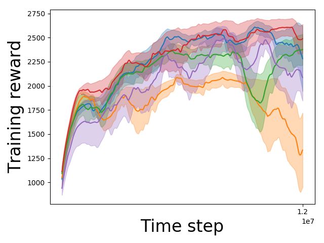
(a) HalfCheetah Train                                   (b) Ant Train

  Figure 2: Fixed gravity setting (−9.81m/s2 ). Training reward for (a) HalfCheetah and (b) Ant.

policy across the different gravity settings across this task, with less potential for transfer between
policies for the various environments. The transferability of policies across different environments and
the effects of the order in which they are encountered are important aspects for future investigation.

               (a) HalfCheetah Train                                   (b) Ant Train

             (c) HalfCheetah Mean Eval                              (d) Ant Mean Eval
Figure 3: Linearly increasing gravity setting. (Top) Training reward for (a) HalfCheetah and (b) Ant.
(Bottom) Mean evaluation reward for (c) HalfCheetah and (d) Ant.

Fluctuating gravity In the fluctuating gravity setting, the performances of the various agents were
less differentiated than in the linearly increasing gravity setting, perhaps because the timescale
of changes to the distribution were shorter and the agents had the opportunity to revisit gravity

                                                   6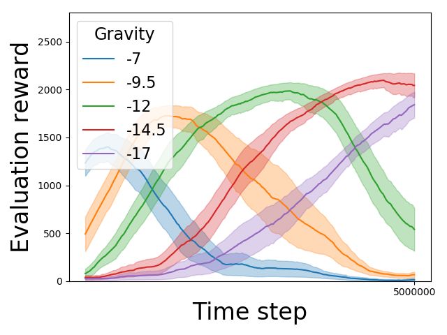
environments (Figure 4). In the HalfCheetah task, the MTR-IRM agent was the best performer in
terms of final training and evaluation rewards, though by a very small margin. In the Ant task, the
best performer was the standard MTR agent, which reached a higher and more stable evaluation
reward than any of the other agents. Once again, as in the linearly increasing gravity setting, the
MTR-IRM agent struggled comparatively on the Ant task.
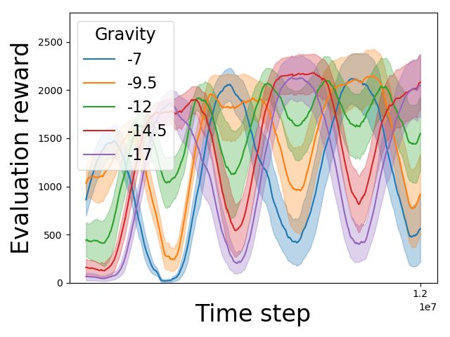
An interesting observation with regards to the agents’ ability to relearn can be made by comparing
the individual evaluation rewards of the FIFO and MTR-IRM agents in the fluctuating gravity setting.
The fluctuating performance on each of the different gravity evaluation settings can be observed
very clearly in the results of the FIFO agent (Figure 5(a)), where the ups and downs in performance
reflect the fluctuations of the gravity setting being trained on. While in the MTR-IRM agent, these
fluctuations in performance can also be observed, the dips in performance on gravity settings that
have not been experienced in a while become significantly shallower as training progresses, providing
evidence that the agent is consolidating its knowledge over time (Figure 5(b)).
(a) HalfCheetah Train (b) Ant Train
(c) HalfCheetah Mean Eval (d) Ant Mean Eval
Figure 4: Fluctuating gravity setting. (Top) Training reward for (a) HalfCheetah and (b) Ant. (Bottom)
Mean evaluation reward for (c) HalfCheetah and (d) Ant.
5 Related Work
Many existing approaches for mitigating catastrophic forgetting in neural networks use buffers for
storing past data or experiences, and are collectively known as replay-based methods [Robins, 1995,
Lopez-Paz et al., 2017, Chaudhry et al., 2019]. Here we briefly elaborate on a selection of works
that investigate or make use of multiple timescales in the replay database, either in continual learning
or in the standard RL setting. In [de Bruin et al., 2015], it is shown that retaining older experiences
as well as the most recent ones can improve the performance of deep RL agents on the pendulum
swing-up task, particularly for smaller replay databases. In [Zhang and Sutton, 2017], it is shown that
combined experience replay, which trains agents on a combination of the most recent experiences
7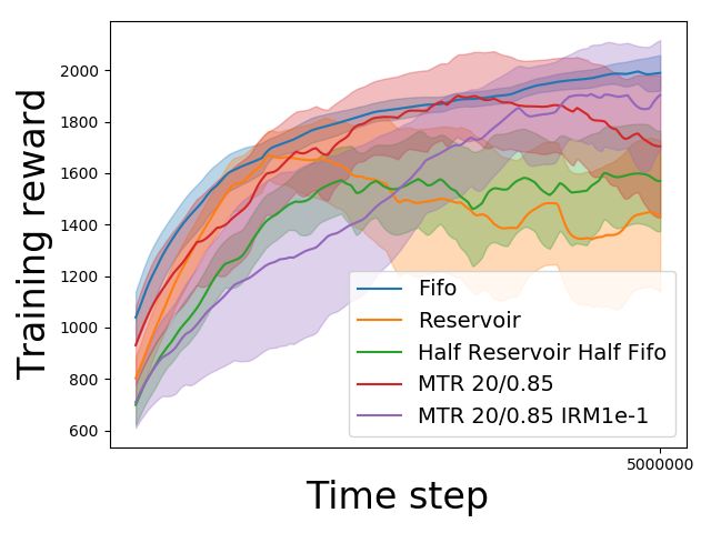
(a) FIFO                                          (b) MTR-IRM
Figure 5: Individual Evaluation rewards for fluctuating gravity HalfCheetah with (a) FIFO buffer and
(b) MTR-IRM buffer.

as they come in and those in the replay buffer, enables faster learning than training on just one or
the other, particularly when the replay database is very large. In [Isele and Cosgun, 2018], various
experience selection methods are evaluated for deep RL, and it was noted that for each method,
a small FIFO buffer was maintained in parallel in order to ensure that the agent did not overfit to
the more long-term memory buffer and had a chance to train on all experiences. In [Rolnick et al.,
2019], it is shown that a 50/50 split of fresh experiences and experiences sampled from a reservoir
buffer provides a good balance between mitigating forgetting and reaching a high overall level of
performance on different tasks in a deep RL setting. As discussed in the Introduction, these methods
employ two different timescales in the distribution of experiences used for training, while the MTR
methods use multiple timescales, which makes them sensitive to changes to the data distribution that
occur at a range of different speeds or frequencies.
In [Wang and Ross, 2019], it is shown that prioritising the replay of recent experiences in the buffer
improves the performance of deep RL agents, using a continuum of priorities across time. In this
paper, a FIFO buffer is used, so the data is only stored at the most recent timescale, but the probability
of an experience being chosen for replay decays exponentially with its age. Other non-replay-based
approaches that use multiple timescales of memory to mitigate catastrophic forgetting in deep RL
include [Kaplanis et al., 2018], which consolidates the individual parameters at multiple timescales,
and [Kaplanis et al., 2019], which consolidates the agent’s policy at multiple timescales, using a
cascade of hidden policy networks.

6   Conclusion
In this paper, we investigated whether a replay buffer set up to record experiences at multiple
timescales could help in a continual reinforcement learning setting where the timing, timescale
and nature of changes to the incoming data distribution are unknown to the agent. One of the
versions of the multi-timescale replay database was combined with the invariant risk minimisation
principle [Arjovsky et al., 2019] in order to try and learn a policy that is invariant across time, with
the idea that it might lead to a more robust policy that is more resistant to catastrophic forgetting.
We tested numerous agents on two different continuous control tasks in three different continual
learning settings and found that the basic MTR agent was the most consistent performer overall.
The MTR-IRM agent was the best continual learner in two of the more nonstationary settings in
the HalfCheetah task, but was relatively poor on the Ant task, indicating that the utility of the IRM
principle may depend on specific aspects of the tasks at hand and the transferability between the
policies in different environments.

Future Work One important avenue for future work would be to evaluate the MTR model in a
broader range of training settings, for example to vary the timescales at which the environment
is adjusted (e.g. gravity fluctuations at different frequencies). Furthermore, it would be useful to
evaluate the sensitivity of the MTR method’s performance to its hyperparameters (βmtr and nb ).

                                                    8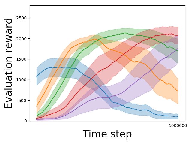
Finally, it is worth noting that, in its current incarnation, the MTR method does not select which
memories to retain for longer in an intelligent way - it is simply determined with a coin toss. In this
light, it would be interesting to explore ways of prioritising the retention of certain memories from
one sub-buffer to the next, for example by the temporal difference error, which is used in [Schaul
et al., 2015] to prioritise the replay of memories in the buffer.

7   Code
The code for this project is available at https://github.com/ChristosKap/multi_timescale_
replay.

References
Continual Learning and Deep Networks Workshop.                https://sites.google.com/site/
  cldlnips2016/home, 2016.
Continual Learning Workshop.         https://sites.google.com/view/continual2018/home,
  2018.
Martin Arjovsky, Léon Bottou, Ishaan Gulrajani, and David Lopez-Paz. Invariant risk minimization.
 arXiv preprint arXiv:1907.02893, 2019.
Arslan Chaudhry, Marcus Rohrbach, Mohamed Elhoseiny, Thalaiyasingam Ajanthan, Puneet K
  Dokania, Philip HS Torr, and Marc’Aurelio Ranzato. Continual learning with tiny episodic
  memories. arXiv preprint arXiv:1902.10486, 2019.
T. de Bruin, J. Kober, K. Tuyls, and R. Babuška. The importance of experience replay database
   composition in deep reinforcement learning. In Deep Reinforcement Learning Workshop, Advances
   in Neural Information Processing Systems (NIPS), 2015.
T. de Bruin, J. Kober, K. Tuyls, and R. Babuška. Off-policy experience retention for deep actor-critic
   learning. In Deep Reinforcement Learning Workshop, Advances in Neural Information Processing
   Systems (NIPS), 2016.
Tuomas Haarnoja, Aurick Zhou, Pieter Abbeel, and Sergey Levine. Soft actor-critic: Off-policy
  maximum entropy deep reinforcement learning with a stochastic actor. In International Conference
  on Machine Learning, pages 1861–1870, 2018a.
Tuomas Haarnoja, Aurick Zhou, Kristian Hartikainen, George Tucker, Sehoon Ha, Jie Tan, Vikash
  Kumar, Henry Zhu, Abhishek Gupta, Pieter Abbeel, et al. Soft actor-critic algorithms and
  applications. arXiv preprint arXiv:1812.05905, 2018b.
Ashley Hill, Antonin Raffin, Maximilian Ernestus, Adam Gleave, Anssi Kanervisto, Rene Traore,
  Prafulla Dhariwal, Christopher Hesse, Oleg Klimov, Alex Nichol, Matthias Plappert, Alec Radford,
  John Schulman, Szymon Sidor, and Yuhuai Wu. Stable baselines. https://github.com/
  hill-a/stable-baselines, 2018.
David Isele and Akansel Cosgun. Selective experience replay for lifelong learning. In Thirty-Second
  AAAI Conference on Artificial Intelligence, 2018.
Michael J Kahana and Mark Adler. Note on the power law of forgetting. bioRxiv, page 173765, 2017.
Christos Kaplanis, Murray Shanahan, and Claudia Clopath. Continual reinforcement learning
  with complex synapses. In Jennifer Dy and Andreas Krause, editors, Proceedings of the 35th
  International Conference on Machine Learning, volume 80 of Proceedings of Machine Learning
  Research, pages 2497–2506, Stockholmsmässan, Stockholm Sweden, 10–15 Jul 2018. PMLR.
  URL http://proceedings.mlr.press/v80/kaplanis18a.html.
Christos Kaplanis, Murray Shanahan, and Claudia Clopath. Policy consolidation for continual
  reinforcement learning. In Kamalika Chaudhuri and Ruslan Salakhutdinov, editors, Proceedings of
  the 36th International Conference on Machine Learning, volume 97 of Proceedings of Machine
  Learning Research, pages 3242–3251, Long Beach, California, USA, 09–15 Jun 2019. PMLR.
  URL http://proceedings.mlr.press/v97/kaplanis19a.html.

                                                  9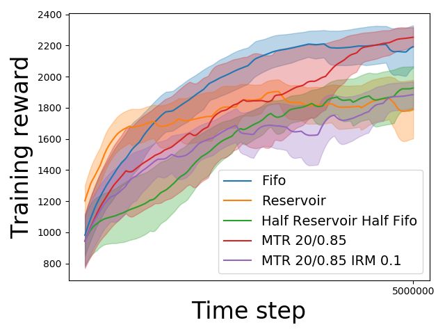
J. Kirkpatrick, R. Pascanu, N. Rabinowitz, J. Veness, G. Desjardins, A. A. Rusu, K. Milan, J. Quan,
   T. Ramalho, A. Grabska-Barwinska, et al. Overcoming catastrophic forgetting in neural networks.
   Proceedings of the National Academy of Sciences, 114(13):3521–3526, 2017.
Timothy P Lillicrap, Jonathan J Hunt, Alexander Pritzel, Nicolas Heess, Tom Erez, Yuval Tassa,
  David Silver, and Daan Wierstra. Continuous control with deep reinforcement learning. arXiv
  preprint arXiv:1509.02971, 2015.
Long-Ji Lin. Self-improving reactive agents based on reinforcement learning, planning and teaching.
  Machine learning, 8(3-4):293–321, 1992.
David Lopez-Paz et al. Gradient episodic memory for continual learning. In Advances in Neural
  Information Processing Systems, pages 6467–6476, 2017.
M. McCloskey and J. N. Cohen. Catastrophic interference in connectionist networks: The sequential
  learning problem. Psychology of Learning and Motivation, 24:109–165, 1989.
V. Mnih, K. Kavukcuoglu, D. Silver, A. A. Rusu, J. Veness, M. G. Bellemare, A. Graves, M. Ried-
   miller, A. K. Fidjeland, G. Ostrovski, et al. Human-level control through deep reinforcement
   learning. Nature, 518(7540):529–533, 2015.
Charles Packer, Katelyn Gao, Jernej Kos, Philipp Krähenbühl, Vladlen Koltun, and Dawn Song.
  Assessing generalization in deep reinforcement learning, 2018.
Mark Bishop Ring. Continual learning in reinforcement environments. PhD thesis, University of
 Texas at Austin Austin, Texas 78712, 1994.
Anthony Robins. Catastrophic forgetting, rehearsal and pseudorehearsal. Connection Science, 7(2):
 123–146, 1995.
David Rolnick, Arun Ahuja, Jonathan Schwarz, Timothy Lillicrap, and Gregory Wayne. Experience
  replay for continual learning. In Advances in Neural Information Processing Systems, pages
  348–358, 2019.
David C Rubin and Amy E Wenzel. One hundred years of forgetting: A quantitative description of
  retention. Psychological review, 103(4):734, 1996.
P. Ruvolo and E. Eaton. Ella: An efficient lifelong learning algorithm. In International Conference
   on Machine Learning, pages 507–515, 2013.
Tom Schaul, John Quan, Ioannis Antonoglou, and David Silver. Prioritized experience replay. arXiv
  preprint arXiv:1511.05952, 2015.
John Schulman, Filip Wolski, Prafulla Dhariwal, Alec Radford, and Oleg Klimov. Proximal policy
  optimization algorithms. arXiv preprint arXiv:1707.06347, 2017.
R. S. Sutton and A. G. Barto. Reinforcement learning: An introduction, volume 1. MIT press
  Cambridge, 1998.
Vladimir Vapnik. Estimation of dependences based on empirical data. Springer Science & Business
  Media, 2006.
Jeffrey S Vitter. Random sampling with a reservoir. ACM Transactions on Mathematical Software
  (TOMS), 11(1):37–57, 1985.
Che Wang and Keith Ross. Boosting soft actor-critic: Emphasizing recent experience without
  forgetting the past. arXiv preprint arXiv:1906.04009, 2019.
John T Wixted and Ebbe B Ebbesen. On the form of forgetting. Psychological science, 2(6):409–415,
  1991.
F. Zenke, B. Poole, and S. Ganguli. Continual learning through synaptic intelligence. In International
   Conference on Machine Learning, pages 3987–3995, 2017.
S. Zhang and R.S. Sutton. A deeper look at experience replay. In Deep Reinforcement Learning
   Symposium NIPS 2017, 2017.

                                                 10
A Appendix
A.1 Linear Gravity Individual Evaluations
In Figure A.1(a), we can see that the cycles of learning and forgetting are quite clear with th FIFO
agent. In all other agents, where older experiences were maintained for longer in the buffer, the
forgetting process is slower. This does not seem to be qualitatively different for the MTR-IRM agent
- it just seems to be able to reach a good balance between achieving a high performance in the various
settings, while forgetting slowly. In particular, it is hard to identify whether there has been much
forward transfer to gravity settings that have yet to be trained on, which one might hope for by
learning an invariant policy: at the beginning of training, the extra IRM constraints seem to inhibit
the progress on all settings (as compared to the standard IRM agent), but in the latter stages the
performance on a number of the later settings improves drastically.
(a) FIFO (b) Reservoir (c) Half Reservoir Half FIFO
(d) MTR (e) MTR with IRM
Figure A.1: Individual Evaluation rewards for linearly increasing gravity HalfCheetah. Mean and
standard error bars over three runs.
A.2 Multi-task (Random gravity) Experiments
A.3 Power Law Forgetting
Several studies have shown that memory performance in humans declines with a power law function
of time [Wixted and Ebbesen, 1991, Rubin and Wenzel, 1996]; in other words, the accuracy on a
memory task at time t is given by y = at−b for some a, b ∈ R+ [Kahana and Adler, 2017]. Here
we provide a mathematical intuition for how the MTR buffer approximates a power law forgetting
function of the form 1t , without giving a formal proof. If we assume the cascade is full, then the
probability of an experience being pushed into the k th sub-buffer is βmtr k−1 , since, for this to happen,
one must be pushed from the 1st to the 2nd with probability βmtr , and another from the 2nd to the
3rd with the same probability, and so on. So, in expectation, nNb · βmtr1k−1 new experiences must be
added to the database for an experience to move from the beginning to the end of the k th sub-buffer.
Thus, if an experience reaches the end of the k th buffer, then the expected number of time steps that
11(a) Training performance (b) Evaluation performance
Figure A.2: Multitask setting: (a) training performance and (b) evaluation performance with uniformly
random gravity between −7 and −17m/s2 with a FIFO buffer. This experiment shows that the agent
has the capacity to represent good policies for all evaluation settings if trained in a non-sequential
setting.
have passed since that experience was added to the first buffer is given by:
k
X N 1
t̂k = E[t|end of k th buffer] = · i−1
(6)
i=1
n b β mtr
N βmtr 1
= · · − 1 (7)
nb 1 − βmtr βmtr k
If we approximate the distribution P(t|end of k th buffer) with a delta function at its mean, t̂k , and
we note that the probability of an experience making it into (k + 1)th buffer at all is βmtr k , then, by
rearranging Equation 7, we can say that the probability of an experience lasting more than t̂k time
steps in the database is given by:
1
P(experience lifetime > t̂k ) = (8)
nb 1−βmtr
t̂k N · βmtr +1
In other words, the probability of an experience having been retained after t time steps is roughly
proportional to 1t .
The expected number of experiences requires to fill up the MTR cascade (such that the size of the
overflow buffer goes to zero) is calculated as follows:
nb
X N 1
· (9)
n βmtr i−1
i=1 b
which for N = 1e6, nb = 20 and βmtr = 0.85, evaluates to 7 million experiences.
A.4 Experimental Details
Gravity settings and baselines The gravity changes in each of the different settings are shown
in Figure A.3. The fixed and linear gravity experiments were run for 5 million time steps, but the
fluctuating gravity was run for 12 million steps, with 3 full cycles of 4 million steps. The value of the
gravity setting was appended to the state vector of the agent so that there was no ambiguity about
what environment the agent was in at each time step.
The MTR and MTR-IRM methods were compared with FIFO, reservoir and half-reservoir-half-FIFO
baselines. In the last baseline, new experiences are pushed either into a FIFO buffer or a reservoir
buffer (both of equal size) with equal probability, and sampled from . The maximum size of each
database used is 1 million experiences and was chosen such that, in every experimental setting, the
agent is unable to store the entire history of its experiences.
12(a) Fixed gravity (b) Linearly increasing gravity (c) Fluctuating gravity
Figure A.3: Gravity settings over the course of the simulation in each of the three set-ups.
Hyperparameters Below is a table of the relevant hyperparameters used in our experiments.
Table 1: Hyperparameters
PARAMETER VALUE
# HIDDEN LAYERS ( ALL NETWORKS ) 2
# UNITS PER HIDDEN LAYER 256
L EARNING RATE 0.0003
O PTIMISER A DAM
A DAM β1 0.9
A DAM β2 0.999
R EPLAY DATABASE SIZE ( ALL BUFFERS ) 1E6
# MTR SUB - BUFFERS nb 20
βmtr 0.85
H IDDEN NEURON TYPE R E LU
TARGET NETWORK τ 0.005
TARGET UPDATE FREQUENCY / TIME STEPS 1
BATCH SIZE 256
# T RAINING TIME STEPS 5 E 6 ( FIXED ), 5 E 6 ( LINEAR ), 1.2 E 7 ( FLUCTUATING )
T RAINING FREQUENCY / TIME STEPS 1
G RAVITY ADJUSTMENT FREQUENCY / TIME STEPS 1000
E VALUATION FREQUENCY / EPISODES 100
# E PISODES PER EVALUATION 1
IRM POLICY COEFFICIENT 0.1
13You can also read