Development of a second-order dynamic stall model
←
→
Page content transcription
If your browser does not render page correctly, please read the page content below
Wind Energ. Sci., 5, 577–590, 2020
https://doi.org/10.5194/wes-5-577-2020
© Author(s) 2020. This work is distributed under
the Creative Commons Attribution 4.0 License.

            Development of a second-order dynamic stall model
                                Niels Adema1 , Menno Kloosterman2 , and Gerard Schepers1
                   1 EUREC   European Master in Renewable Energy, Hanze University of Applied Sciences,
                                           Groningen, 9747 AS, the Netherlands
                                      2 DNV GL, Groningen, 9743 AN, the Netherlands

                               Correspondence: Niels Adema (nielsadema1994@gmail.com)

                                Received: 14 November 2019 – Discussion started: 4 December 2019
                              Revised: 2 April 2020 – Accepted: 9 April 2020 – Published: 15 May 2020

       Abstract. Dynamic stall phenomena carry the risk of negative damping and instability in wind turbine blades.
       It is crucial to model these phenomena accurately to reduce inaccuracies in predicting design driving (fatigue
       and extreme) loads. Some of the inaccuracies in current dynamic stall models may be due to the fact that they
       are not properly designed for high angles of attack and that they do not specifically describe vortex shedding
       behaviour. The Snel second-order dynamic stall model attempts to explicitly model unsteady vortex shedding.
       This model could therefore be a valuable addition to a turbine design software such as Bladed. In this paper
       the model has been validated with oscillating aerofoil experiments, and improvements have been proposed for
       reducing inaccuracies. The proposed changes led to an overall reduction in error between the model and exper-
       imental data. Furthermore the vibration frequency prediction improved significantly. The improved model has
       been implemented in Bladed and tested against small-scale turbine experiments at parked conditions. At high
       angles of attack the model looks promising for reducing mismatches between predicted and measured (fatigue
       and extreme) loading, leading to possible lower safety factors for design and more cost-efficient designs for
       future wind turbines.

1   Introduction                                                    uate, 2007). Therefore, accurate modelling of dynamic stall
                                                                    is therefore crucial in wind turbine design (Choudry et al.,
Wind turbines operate in highly unsteady aerodynamic en-            2014).
vironments (Leishman, 2002). For design and certification,             Dynamic stall is a phenomenon leading to larger varia-
design load cases (DLCs) have been set which describe               tions in lift, drag, and pitching moments on the aerofoil than
the conditions that wind turbine designs have to withstand          would be observed during steady operation (Choudry et al.,
(DNV GL, 2016). Some of the design driving DLCs are                 2014). This then creates larger aerodynamic forces on the
those for parked and idling conditions where wind turbine           blades than expected during steady conditions (Leishman,
blades will experience high angles of attack (AoAs), leading        2002). Dynamic stall happens with dynamic variation in the
to (dynamic) stall behaviour (Schreck et al., 2000). The wind       inflow and/or the effective angle of attack and can be viewed
turbine yaw angle is defined as the angle in the horizontal         as a delay in the onset of stall. Recirculation of flow after
plane between the free-stream wind direction and the wind           the static stall angle starts near the trailing edge and rapidly
turbine rotor shaft. It can be noted that when the turbine is       moves towards the leading edge, leading to the formation of a
parked, and the blades are pitched to 90◦ , the yaw angle ef-       large dynamic stall clockwise vortex at the leading edge at in-
fectively becomes the inflow angle. When the yaw system is          creasing angles of attack. The dynamic stall vortex will travel
not operating during parked conditions due to a failure, the        along the suction side, leading towards the trailing edge be-
blades will experience flow from all directions. For particular     fore detaching completely. Full separation will occur when
wind directions the flow on the blades is separated, leading        the dynamic stall vortex is completely detached. This mo-
to dynamic stall effects. These effects may already appear          ment is called the “break” or “dynamic stall onset”. As a re-
at inflow angles of below 30 and 20◦ (Gonzalez and Mund-

Published by Copernicus Publications on behalf of the European Academy of Wind Energy e.V.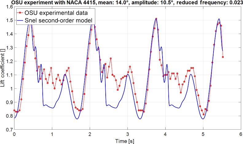
578                                                     N. Adema et al.: Development of a second-order dynamic stall model

sult, low lift remains until reattachment of the flow. However,    angles of attack and that there are some of them that do
a time delay for reattachment of the flow is present as well.      not specifically describe vortex shedding behaviour. The Snel
After reattachment the process repeats, creating a hystere-        second-order dynamic stall model does attempt to explicitly
sis loop. Dynamic stall phenomena carry the risk of negative       model unsteady vortex shedding. However, there is still the
damping and instability, especially if the aerofoil is oscillat-   need for further tuning and validation of the model (Snel,
ing in and out of stall (McCroskey, 1981). A visual descrip-       1997). Snel takes the model from Truong (1993) as a start-
tion for dynamic stall is presented in Fig. 1.                     ing point. Truong (2017) already showed promise by modify-
   When keeping the aerofoil pitched in (deep) stall for           ing his model for unsteady vortex shedding, and Snel takes a
longer periods of time, periodic vortex shedding will occur.       similar approach. However, as described in Sect. 2, the Snel
A single large dynamic stall vortex will no longer be shed,        model differs from the Truong model by incorporating the
but rather multiple periodic vortices from both the leading        steady lift coefficient and is therefore interesting to study
and trailing edge will be shed. This will induce time-varying      and modify. This paper will provide a detailed analysis of
loads on the blades (Riziotis et al., 2010). The periodic vortex   the Snel second-order model and will try to answer the fol-
shedding is characterized by the Strouhal number represent-        lowing main research question:
ing the dimensionless frequency of shedding (Pellegrino and        what are possible ways to improve predictions of blade vi-
Meskell, 2013). The Strouhal number is defined following           brations during dynamic stall in parked conditions using the
Eq. (1):                                                           Snel second-order model?
                                                                      This paper will have the following outline.
       f ·c
St =        ,                                               (1)
        U                                                              – The Snel model is validated against experimental data.
in which f notes the characteristic vortex shedding fre-               – Proposed changes are presented based on the validation
quency, c the aerofoil chord (sometimes the projected chord              results to improve the model predictions. These include
length perpendicular to the incoming flow), and U the wind               a dimensional analysis, calculation of the slope for the
velocity at the wind turbine blade section. Synchronization              potential lift coefficient, application of the normal force
of the natural and Strouhal frequencies (a “lock-in”) will               coefficient, an investigation into the downstroke and
lead to resonance (Pellegrino and Meskell, 2013). Locked-in              vortex shedding predictions of the model, and finally an
vortex-induced vibrations are a potential threat in standstill           optimization for empirical constants.
conditions as the turbine size is increasing. Modern aeroe-
lastic tools with dynamic stall models are only able to pro-           – Attention will be paid to vibration prediction as this in-
vide accurate deep stall loads at conditions close to maxi-              fluences turbine fatigue loading, which has a large im-
mal lift, so relatively small angles of attack (Riziotis et al.,         pact on the design of the wind turbine.
2010). The same study noted that today’s aeroelastic tools
are not properly tuned for high angles of attack. Mismatches           – An absolute error analysis is carried out before and af-
between load predictions between measurements and engi-                  ter the improvements to quantify the increase in perfor-
neering tools have been found to be as high as 20 % for high-            mance.
wind-speed dynamic stall conditions (Schreck, 2002). State-            – The improved model will be tested with actual small-
of-the-art aerodynamic models overestimate fatigue loading               scale turbine experimental data to assess performance
by 15 % (Schepers and Snel, 2007). Madsen et al. (2019)                  in combination with Bladed.
show promise for using computational fluid dynamics (CFD)
in early stages of wind turbine design and shape optimiza-
                                                                   2    Analysis and validation of the Snel second-order
tion, and Sørensen et al. (2016) showed that CFD models had
                                                                        model
good agreement with instrumented rotor experiments. So al-
though CFD is becoming more available and useful in wind           This section will validate the Snel model and propose adap-
turbine design, it requires large computational power. There-      tations to the model to improve the performance. The de-
fore these tools are not yet fit for practical design calcula-     scription of the model is based on the description in both
tions. In the industry there is a need for relatively fast and     Snel (1997) and Hollierhoek et al. (2013). Snel (1997)
accurate engineering models predicting key loading. Hol-           derived a dynamic stall model based on the work of
lierhoek et al. (2013) studied different dynamic stall mod-        Truong (1993), who proposed that the dynamic lift coef-
els, namely Beddoes–Leishman, ONERA, and Snel models.              ficient can be distinguished into two parts, namely 1cl1
However, a clear single best model was not found. Gonzalez         and 1cl2 :
and Munduate (2007) and Wala et al. (2018) both showed
promising results using modified and optimized Beddoes–            cl,dyn = cl,steady + 1cl1 + 1cl2 .                           (2)
Leishman models compared with experimental data. Inac-
curacies in dynamic stall models may be due to the above-          The first describes the forcing frequency response and the
described fact that they are not properly designed for high        second term the self-exited higher-frequency dynamics. Snel

Wind Energ. Sci., 5, 577–590, 2020                                                      https://doi.org/10.5194/wes-5-577-2020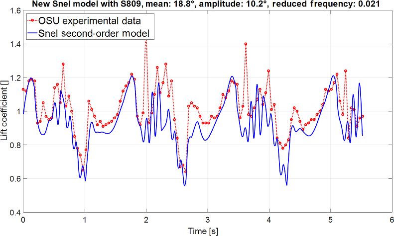
N. Adema et al.: Development of a second-order dynamic stall model                                                                    579

Figure 1. Classical visual representation of dynamic stall (Leishman, 2002).

follows this approach but also expresses the first part as the          non-dimensional by taking the coefficient of the derivative
difference from the steady-state (time-averaged) lift coeffi-           term as the time constant usually used in dynamic stall. This
cient (Montgomerie, 1996). The dynamic lift of the Snel                 constant is described in Eq. (11).
model will be as in Eq. (2). The first part, 1cl1 , must de-
cay to zero when no excitation is present, while the second             ft1 = τ 1ċl,pot                                              (4)
part will decay to zero for small angles of attack, but nearing         1cl,pot = cl,pot − cl,steady = 2π sin (α − α0 ) − cl,steady   (5)
stall the second part will show periodic oscillations related to
vortex shedding.                                                        The coefficient of 1cl1 can be seen as a spring trying to pull
   In the original model of Truong the first part is based              the term back to the steady state. The stiffness of the spring
on the Beddoes–Leishman dynamic stall model. The Snel                   of this equation is given by Eq. (6). In downwards pitching
model uses the SIMPLE model from Montgomerie (1996)                     motion the stiffness is higher than in upwards pitching mo-
as a departure point for the first-order correction while               tion.
Truong (1993) uses the Beddoes–Leishman (B–L) model to                          ( 1+0.51c
                                                                                           l,pot
                                                                                                 if α̇cl,pot ≤ 0
calculate 1cl1 . The modelling of the first part will therefore                     8(1+60τ α̇)
                                                                        cf10 =     1+0.51cl,pot                                    (6)
follow                                                                              8(1+80τ α̇)  if α̇cl,pot > 0

τ 1cl1 + cf10 1cl1 = ft1 .                                     (3)      The second part of the dynamic lift coefficient is of the sec-
                                                                        ond order to create the higher-frequency dynamics. This will
The forcing term ft1 will be based on the time derivative of            be a non-linear mass–damper–spring system following
the difference between the steady and potential lift coeffi-
cients. This is shown in Eqs. (4) and (5). The function is made         τ 2 1c̈l2 + cf21 1ċl2 + cf20 1cl2 = ft2 .                    (7)

https://doi.org/10.5194/wes-5-577-2020                                                            Wind Energ. Sci., 5, 577–590, 2020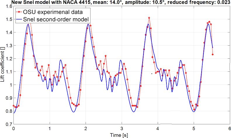
580 N. Adema et al.: Development of a second-order dynamic stall model
The spring and damping coefficients are taken from Table 1. Selected cases from the OSU experiments.
Snel (1997) and are defined as in Eqs. (8) and (9) respec-
tively. Aerofoil No. of Mean Average Amplitude Oscillation
test wind angle of (◦ ) frequency
h 2 i h i cases speed attack (Hz)
cf20 = ks2 1 + 3 1cl2 1 + 3α̇ 2 (8) (m s−1 ) (◦ )
cf21 = 1 42.8 8.1 10.2 0.60
( h 2 i 2 43.0 8.2 10.1 1.20
60τ ks −0.01 1cl,pot − 0.5 + 2 1cl2 if α̇ > 0 (9) 3 42.7 8.3 10.2 1.89
2τ ks if α̇ ≤ 0 4 42.8 13.2 10.4 0.60
S809 5 41.7 12.9 10.1 1.22
6 42.0 12.9 10.1 1.81
Also, here it can be noted that the response will be different in 7 42.3 18.8 10.2 0.61
pitching upwards or downwards. The forcing term is defined 8 42.1 18.8 10.1 1.18
as 9 42.6 18.7 10.0 1.84
11 37.9 7.0 11.2 0.61
ft2 = 0.1ks −0.151cl,pot + 0.051ċl,pot . (10) 12 37.9 7.5 10.8 1.20
13 37.8 7.3 10.7 1.85
In the second-order part of the model, ks is taken as the re- 14 37.8 14.0 10.5 0.60
duced vortex shedding frequency or Strouhal number. This is NACA 4415 15 37.7 14.1 10.6 1.22
16 37.3 14.1 10.6 1.81
given a value of 0.2 as in the original model (Snel, 1997). In
17 37.2 18.6 10.5 0.61
the above equations the time constant is given below and can 18 37.1 18.3 10.8 1.24
be seen as the time it takes for the wind to travel half a chord 19 37.2 18.4 10.7 1.84
distance:
τ = c/2U. (11) – The shedding frequency is not dependent on the reduced
frequency while the experiments do show a dependency.
2.1 Initial model implementation and validation
These points will be analysed as part of the possible improve-
The Snel model as described in the section above is imple- ments described in Sect. 3.3 up to Sect. 3.9.
mented in a MATLAB environment. The numerical imple-
mentation follows the steps described in De Vaal (2009).
2.2 Error analysis
The time step used is 0.001 s to capture higher-frequency
events from the Ohio State University experiments. The Ohio To quantify the accuracy of the Snel model, the total absolute
State University (OSU) experiments (Hoffmann et al., 1996) error between model predictions and experimental data is
will be used for validation of the initial implementation of calculated. This will give an objective measure to assess pro-
the Snel model. In the OSU experiments an extensive set of posed improvements. The Snel model is interpolated along
aerofoils have been tested for both unsteady and steady data. the angle of attack to obtain the dynamic lift coefficient out-
The measurements recorded responses to forced sinusoidal put at the precise angles of attack of the OSU experiment.
pitching oscillations. Different amplitudes, mean angles of The errors are then evaluated according to
attack, oscillation frequencies, and Reynolds numbers were
tested. The focus in this paper will be on the NACA4415 Ei = cl,model (αi ) − cl,OSU (αi ) , (12)
and S809 aerofoils. The model parameters obtained from the
OSU database, as displayed in Table 1, will be analysed. The and the total absolute error of all data points is calculated
oscillation frequencies of the cases are set such that the forc- using
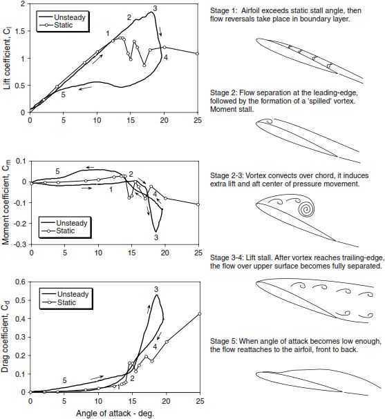
ing angle of attack matches the OSU experiments. Figures 2 v
u n
and 3 show the time series of the lift coefficient for cases u1 X 2
absolute error = t E , (13)
with both low and high reduced frequencies and low and high n i=1 i
mean angles of attack. The following observations can been
made for the current model: in which n denotes the number of data points of the OSU
– The current model overpredicts the loss of lift during experimental data.
the downstroke.
3 Proposed changes to the Snel model
– The predicted vortex shedding does not always happen
at the correct time. This section will outline proposed modifications to the Snel
model. The following areas will be investigated for modifi-
– There is currently no unsteady vortex shedding at higher
cation:
angles of attack.
Wind Energ. Sci., 5, 577–590, 2020 https://doi.org/10.5194/wes-5-577-2020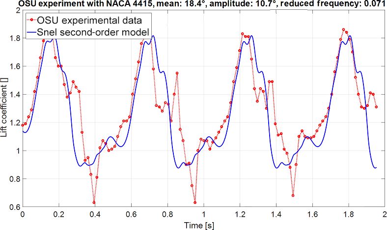
N. Adema et al.: Development of a second-order dynamic stall model                                                                    581

Figure 2. Lift coefficient time of the initial Snel model (NACA 4415 aerofoil with mean angle of attack of 14◦ , amplitude of 10.5◦ , and
reduced frequency of 0.023).

Figure 3. Lift coefficient time of the initial Snel model (NACA 4415 aerofoil with mean angle of attack of 18.4◦ , amplitude of 10.7◦ , and
reduced frequency of 0.071).

  – a dimensional analysis of the model,                                3.1   Dimensional analysis
  – the calculation method of the slope for the potential lift          It can be seen in the formulation of the model that Eqs. (8)
    coefficient,                                                        and (10) are cast in a dimensional form. For different values
                                                                        for chords, wind speed, and pitching frequency, the current
  – application of the normal force coefficient instead of the
                                                                        model will not produce identical results. In order to make
    lift force coefficient,
                                                                        them dimensionless, the time constant used in dynamic stall
  – the downstroke prediction of the model,                             (Eq. 11) is added. The new constants will be such that the
                                                                        initial value of the constant is kept. The equations will now
  – prediction of vortex shedding,                                      be
  – and lastly an optimization for empirical (aerofoil-
    specific) constants.

https://doi.org/10.5194/wes-5-577-2020                                                           Wind Energ. Sci., 5, 577–590, 2020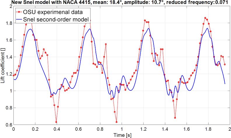
582 N. Adema et al.: Development of a second-order dynamic stall model
downstroke. To improve this behaviour the forcing term is set
h 2 i h i
cf20 = ks2 1 + 3 1cl2
1 + 280 τ α̇ ,2 2 2
(14) to zero for the downstroke. In addition, Figs. 2 and 3 show
that the predicted shedding in the upstroke is larger than in
ft2 = 0.1ks −0.151cl,pot + 8τ 1ċl,pot . (15) the measurements. Therefore, the forcing term is lowered and
will be changed to
ft2 = 0.1ks −0.081cl,pot + 1.5τ 1ċl,pot . (20)
3.2 Correct slope for Cl potential
From Figs. 1 and 2 it is visible that there are higher frequen-
The Snel model uses 2π as theoretical slope for lift coef- cies in the downstroke. This is not modelled as cf21 is a con-
ficient at low angles of attack. This theoretical value might stant value in the downstroke; see Eq. (9). To allow shedding,
not be applicable to real aerofoils. Calculating the precise the coefficient is changed to
slope improves the accuracy of the model. Therefore the
slope calculated from the aerofoil polar is used in the model. cf21 =
The slope is calculated between the intercept at angle of at-
h i
60τ ks −0.01 1cn,pot − 0.5 + 2 1cn 2
2 if α̇ > 0
tack = 0 and the intercept at lift coefficient = 0. h i . (21)
60τ ks −0.01 1cn,pot − 0.5 + 12 1cn 2
2 if α̇ ≤ 0
3.3 Application of the normal force coefficient
The damping in the downstroke is set higher than in the up-
The Snel model uses the lift coefficient of the steady aerofoil stroke.
data. However, the lift coefficient tends to zero when angles
of attack reach 90◦ . At a 90◦ angle of attack there is still 3.5 Prediction of vortex shedding
unsteady vortex shedding present. Therefore, it would make
sense to model vortex shedding to the normal force on the The shedding frequency will depend on the angle of attack.
aerofoil instead of the lift force. The normal force coefficient The current model does not predict a dependency and so it
together with the lift and drag coefficients are presented in has to be improved in this aspect. The Strouhal number uses
Fig. 4. For implementation all the CL terms are changed to the chord or the projected chord perpendicular to the incom-
Cn terms. A couple of additions must then be made to the ing flow. Because the projected chord length is driven by the
model to obtain the dynamic lift and drag coefficients. First, angle of attack, it is proposed to add the projected chord
the steady normal force coefficient (cn,steady ) is the sum of length to the “spring” term (cf20 ) of the second-order part.
the steady lift and drag coefficient and the angle of attack This allows for the desired dependency of stiffness. From
following Eq. (1) it can be inferred that when projecting the chord per-
pendicular to the incoming flow this is effectively the same
cn,steady = cl,steady cos(α) + cd,steady sin(α), (16) as projecting the Strouhal number. The new equation for cf20
will now be
and the steady chordwise coefficient (cc,steady ) will follow h 2 i h i
2
cf20 = 10 · ks,pr 1 + 3 1cl2 1 + 2802 τ 2 α̇ 2 , (22)
cc,steady = −cl,steady sin(α) + cd,steady cos(α). (17)
with
When the dynamic normal force coefficient has been ob-
tained, an inverse calculation yields the lift and drag coef- ks,pr = ks · sin(α). (23)
ficients:
cl,dyn = cn,dyn cos(α) − Cc,steady sin(α), (18)
cd,dyn = cn,dyn sin(α) + Cc,steady cos(α). (19) 3.6 Optimization for (aerofoil-specific) constants
An unconstrained minimization algorithm in MATLAB is
3.4 Downstroke of the model
used to optimize empirical constants. The algorithm searches
The consistent differences between the implementation of for the lowest summation of the absolute errors, from
the Snel second-order model and earlier implementations are Eq. (13), of all cases considered. The constants selected for
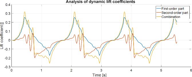
lower values in the downstroke. Figure 5 shows the first- and this analysis are shown in the initial row of Table 2. The
second-order part of the model as a function of time. The constants are selected since they are included in equations
second-order part (1cl2 ) contributes highly to the lower val- affected by the modifications from this section and also be-
ues at the start of the downstroke, which causes a large part cause they have a high influence on the output of the Snel
of the observed error. model. Three optimization analyses have been carried out:
Equation (10) uses −0.151cl,pot . Together with a negative a global optimization which covers all cases, an optimiza-
1ċl,pot in the downstroke, ft2 will be highly negative in the tion which focussed only on the cases with a mean angle of
Wind Energ. Sci., 5, 577–590, 2020 https://doi.org/10.5194/wes-5-577-2020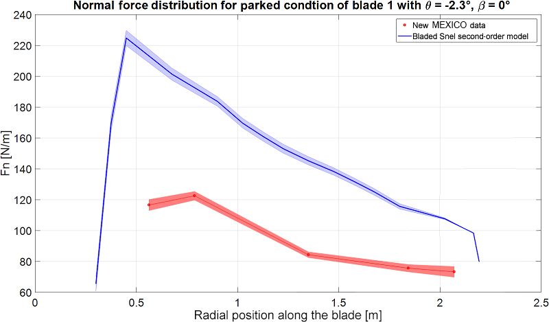
N. Adema et al.: Development of a second-order dynamic stall model 583
Figure 4. Steady polars of the NACA 4415 aerofoil.
Figure 5. Analysis of the dynamic lift coefficient.
attack of 14 or 20◦ , and an optimization on the low-reduced- As a result of this optimization step the following changes
frequency cases. The initial constants as in Table 2 are the are implemented. Equation (6) will change to
start values for the optimization. The results for all individ- ( 1+C ·1c
1 n,pot
ual cases, using the error analysis described in Sect. 2.2, are 8(1+60τ α̇) if α̇cn,pot ≤ 0
shown in Fig. 6. It can be seen that the global optimiza- cf10 = 1+C1 ·1cn,pot . (24)
8(1+80τ α̇) if α̇cn,pot > 0
tion is the most optimal. The global optimization gives the
most consistently lower error compared to the initial model. Equation (20) will change to
In Bladed the Beddoes–Leishman dynamic stall model has
three sensitive constants which are allowed to be changed ft2 = 0.01ks −0.041cn,pot + C2 τ 1̇cn,pot . (25)
by the user. For the Snel model, the optimization shows that
two constants are the most sensitive. The optimization out- The first-order coefficient C1 will be 0.5 for the NACA 4415
put showed significantly different values for these constants aerofoil and 0.2 for the S809. For the second-order forcing
for the NACA 4415 and the S809 aerofoils. They are shown coefficient C2 will be 1 and 1.5 respectively. Table 2 shows
in the improved row of Table 2. These constants must be al- that for Eqs. (18) and (19) the constants remain the same.
lowed to be changed by users of a turbine design code. The Therefore these remain unchanged. Finally Eq. (21) will be-
same goes for the Strouhal number. The constants are come as follows:
– C1 from Table 2, which will be called the first-order cf21 =
coefficient and
h i
60τ ks −0.01 1cn,pot − 0.5 + 2 1cn 2
2 if α̇ > 0
h i . (26)
60τ ks −0.01 1cn,pot − 0.5 + 14 1cn 2
– C2 from Table 2, which will be called the second-order 2 if α̇ ≤ 0
forcing coefficient.
https://doi.org/10.5194/wes-5-577-2020 Wind Energ. Sci., 5, 577–590, 2020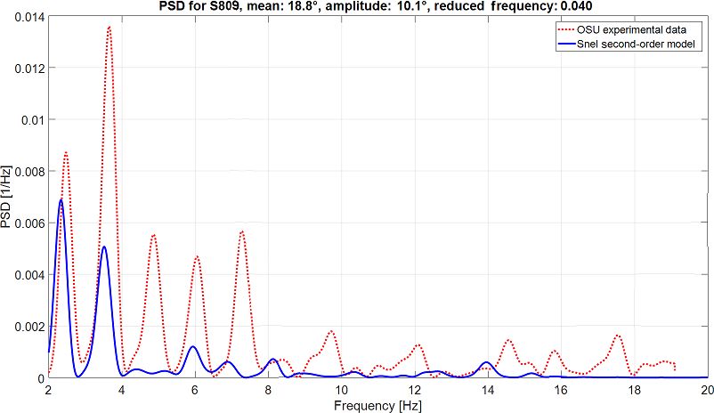
584                                                         N. Adema et al.: Development of a second-order dynamic stall model

Table 2. Constants used for optimization.

                              Equation      (6)                        (20)                      (22)     (21)      (21)
                                                                                                                 downstroke
                              Initial       0.5              0.1   −0.08      1.5           10      280   60        12
                 Constant     Improved      0.2; 0.5 (C1)   0.01   −0.04      1.5; 1 (C2)   10      280   60        14

Figure 6. Absolute error analysis of the optimization runs for all cases from Table 1.

Figure 7. Lift coefficient over time of the improved Snel model (NACA 4415 aerofoil with mean angle of attack of 14◦ , amplitude of 10.5◦ ,
and reduced frequency of 0.023).

4   Results of the proposed modifications                                tures the shedding slightly better, even though there is less
                                                                         shedding present. Furthermore, it can be seen that the fre-
                                                                         quency changes between both cases as desired. It is impor-
The modified Snel model is implemented as described in
                                                                         tant to investigate the impact changes on different situations
Sect. 2.1 and tested against the same set of experiments as
                                                                         and aerofoils. Figure 9 displays the updated model in com-
in Table 1. The results of the modified Snel model are shown
                                                                         bination with the S809 aerofoil. The improved model still
in Figs. 7 and 8. In comparison to Figs. 2 and 3 it is noted
                                                                         predicts slightly lower values than the experiments but the
that the shedding prediction at low reduced frequency is im-
proved. For the higher reduced frequency the model also cap-

Wind Energ. Sci., 5, 577–590, 2020                                                               https://doi.org/10.5194/wes-5-577-2020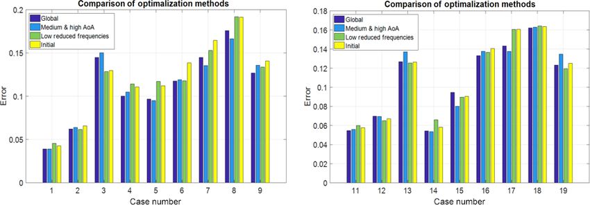
N. Adema et al.: Development of a second-order dynamic stall model                                                                     585

Figure 8. Lift coefficient over time of the improved Snel model (NACA 4415 aerofoil with mean angle of attack of 18.4◦ , amplitude of
10.7◦ , and reduced frequency of 0.071).

Figure 9. Lift coefficient over time of the improved Snel model (S809 aerofoil with mean angle of attack of 18.8◦ , amplitude of 10.2◦ , and
reduced frequency of 0.021).

overall trends are followed nicely, and shedding frequency              cies are higher and the forcing frequency will take up a large
matches the experiment well.                                            proportion of the PSD. The results for both aerofoils are
   Another goal of the proposed changes to the Snel model               shown in Figs. 10 and 11. From the figures it becomes clear
was to capture, predict, and match the vortex shedding and              that the Snel model captures, for both aerofoils at different
the shedding frequency of aerofoils in dynamic stall condi-             mean angles of attack and different reduced frequencies, the
tions. In order to check the validity of these changes in a             self-induced shedding frequencies fairly correct. However,
quantitative way, a frequency domain analysis has been per-             as shown in Figs. 7–9, there is still room for improvement
formed. The power spectral density (PSD) estimate is cal-               here. All predicted shedding frequencies match frequencies
culated using Welch’s method. The Hamming window is set                 observed in the measurements, whereas the intensity is not
equal to the number of data points and the number of over-              always correct. Care must be taken with the higher frequen-
lapped values to 50 % of the window length. The forcing fre-            cies as the OSU measurement has a relatively low sampling
quency is removed from the plot as the shedding frequen-

https://doi.org/10.5194/wes-5-577-2020                                                            Wind Energ. Sci., 5, 577–590, 2020
586                                                      N. Adema et al.: Development of a second-order dynamic stall model

Figure 10. Power spectral density of experimental data and the improved Snel model (NACA 4415 aerofoil mean angle of attack of 14◦ ,
amplitude of 10.5◦ , and reduced frequency of 0.023).

Figure 11. Power spectral density of experimental data and the improved Snel model (S809 aerofoil with mean angle of attack of 18.8◦ ,
amplitude of 10.1◦ , and reduced frequency of 0.040).

frequency and might therefore not fully capture some higher-         changes developed and presented in this paper improve the
frequency dynamics.                                                  performance of the Snel second-order model.
   To quantify the improvements, the effects of all previous
changes on the overall absolute error of the new model are
shown in Fig. 12 together with the overall error of the initial      5   The updated Snel model performance with New
model of Sect. 3. It is seen that the improved model outper-             MEXICO data
forms the initial model in almost every case with a single ex-
ception. The initial model already gave very accurate results        Model Experiments In Controlled Conditions (MEXICO)
for that case, and the increase in error is very small com-          was a project in which an instrumented, three-bladed tur-
pared to the reduction achieved in all other cases. It is also       bine of 4.5 m rotor diameter was tested (Schepers et al.,
noted that the overall prediction of the shedding phenomena          2012). MEXICO was carried out in the Large Low-Speed
has been improved. Hence it can be concluded that the model          Facility (LLF) of the German-Dutch Wind Tunnels (DNW)
                                                                     (Schepers et al., 2012). The blades were fitted with pres-

Wind Energ. Sci., 5, 577–590, 2020                                                       https://doi.org/10.5194/wes-5-577-2020
N. Adema et al.: Development of a second-order dynamic stall model 587 Figure 12. Comparison of the total absolute error of both the initial and improved Snel models. Figure 13. Normal force distribution of the blade at 0◦ azimuth with −2.3◦ pitch and 0◦ wind direction. The bold line represents the mean value, and the shaded area is the standard deviation. sure sensors at 25 %, 35 %, 60 %, 82 %, and 92 % radial to New MEXICO data. The modal damping in the calcula- positions. Tests were performed with 30 m s−1 wind speed, tions is set to 0.5 %. In the runs the rotational augmentation blades pitched to vane, and yaw inflow angles in the range is turned off just like in Khan (2018). The tip and root loss of −90 to 30◦ and for three azimuthal positions (0, 120, and Prandtl corrections as well as tower shadow effects are also 240◦ ). This data set is particularly valuable for the testing of turned off. A total of 21 blade stations, as in the geometry dynamic stall models as it represents standard load cases set description of the New MEXICO blade, are used. The start- out by the IEC (DNV GL, 2016). For a complete overview of ing and ending radii for the dynamic stall model are 25 % the MEXICO and New MEXICO projects, reference is made and 95 %. The normal force distribution in axial flow, with to Schepers et al. (2012). Khan (2018) conducted similar re- pitch −2.3◦ and thus an angle of attack of about 90◦ , is given search with different dynamic stall models, and their study in Fig. 13. The Snel model shows roughly the same size of will be used as a baseline in this paper. The improved Snel normal force fluctuations as in the experiment. Khan (2018) model from this paper will be tested against the New MEX- found similar deviations in the mean values of the normal ICO data sets of Table 3 (β = wind direction, θ = pitch angle) force distributions with different turbine design codes and to see if the additions and changes to the model have a pos- different dynamic stall models. A reason for this deviation itive influence on the accuracy. The blade geometry, mass, is not mentioned and should be part of further research. The and flexibility distribution are modelled in Bladed according improved Snel model predicts shedding at −2.3◦ pitch with https://doi.org/10.5194/wes-5-577-2020 Wind Energ. Sci., 5, 577–590, 2020
588                                                       N. Adema et al.: Development of a second-order dynamic stall model

Figure 14. Power spectral density at 82 % span of the blade at 0◦ azimuth with −2.3◦ pitch and 0◦ wind direction.

Figure 15. Normal force distribution of the blade at 120◦ azimuth with 90◦ pitch and 30◦ wind direction. The bold line represents the mean
value and the shaded area the standard deviation.

axial flow, due to the addition of the normal force coefficient,       ICO blade. Figure 15 shows the normal force distribution for
while the original model as in Khan (2018) does not. The               the blade at azimuth 120◦ for the yawed case with 30◦ wind
PSDs of the time series of both the New MEXICO data and                direction and 90◦ pitch. Interesting to notice for this case is
the Bladed output are compared. The normal force time se-              that the angle of attack will be negative. The Snel model does
ries are standardized by subtracting the mean and dividing by          not show any unsteadiness in the normal force distribution.
the standard deviation. The Hamming window is set to equal             Further research is needed to explain and improve the Snel
the number of data points and the number of overlapped val-            model for negative angles of attack.
ues to 50 % of the window length. The results are shown in                A single reason for the higher-frequency prediction has
Fig. 14 at the radial location of 82 % of the total span.              not been found. Several possibilities are suggested. First, the
   The updated Snel model shows significantly higher-                  modal damping is not specified in the New MEXICO turbine
frequency vibrations in the normal force of the New MEX-               data and was therefore assumed to be 0.5 %. Second, the im-

Wind Energ. Sci., 5, 577–590, 2020                                                          https://doi.org/10.5194/wes-5-577-2020
N. Adema et al.: Development of a second-order dynamic stall model                                                                   589

Table 3. Investigated cases from the New MEXICO experiments.

                       Case    Case type                         Data point      U           β         2
                       no.                                                     (m s−1 )     (◦ )      (◦ )   (rpm)
                       1                                               372       ±30          0       90      0
                       2                                               382       ±30          0       75      0
                       3       Standstill with axial flow              373       ±30          0       45      0
                       4       (rough)                                 386       ±30          0       30      0
                       5                                               400       ±30          0       12      0
                       6                                               375       ±30          0     −2.3      0
                       7                                    405, 406, 407        ±30       −90        90      0
                       8                                    408, 409, 410        ±30       −60        90      0
                       9       Standstill with yawed flow   411, 412, 413        ±30       −45        90      0
                       10      (rough)                      414, 415, 416        ±30       −30        90      0
                       11                                   420, 421, 422        ±30        15        90      0
                       12                                   423, 424, 425        ±30        30        90      0

pact of different aerofoils from the New MEXICO blade is              tions presented in this paper. The main difference lies in the
unknown. The first-order or second-order forcing coefficients         incorporation of the steady lift data as described in Sect. 2.
might require other values. Furthermore, the Strouhal num-            The authors highly recommend a study comparing both the
ber for the New MEXICO blade is not 0.2 Hz at high angles             model described in Truong (2017) and the model presented in
of attack (Khan, 2018). Research by Skrypinski et al. (2014)          this paper. The model as proposed is formulated on the basis
and Zou et al. (2015) shows that for aerofoils with an effec-         of variations in angles of attack. It is recommended for fur-
tive angle of attack of around 90◦ the Strouhal number should         ther research to delve into the possibility to adept this model
be around 0.10–0.13 Hz. This ought to be implemented in the           to dynamic variation in inflow velocity for the case of rotat-
model and tested in further research. Third, wind tunnel ef-          ing and vibrating blades.
fects are not modelled in Bladed. The wind field in Bladed               The proposed Snel second-order dynamic stall model
has zero turbulence and wind tunnel effects. More research            might become a valuable addition to the modelling of dy-
on the Snel model in Bladed with actual turbine data is ad-           namic behaviour in stall conditions. As the conditions tested
vised.                                                                in this paper are often design driving, the Snel model looks
                                                                      promising for more accurate prediction of design-driving (fa-
                                                                      tigue and extreme) loads and more cost-efficient wind turbine
6   Conclusion and recommendations                                    designs.

The Snel model has been validated with OSU experimental
data, and following this validation propositions for improve-         Code and data availability. The paper uses the publicly avail-
ments have been made. The improvements to the model have              able OSU oscillating aerofoil experiment data. The implementation
been tested and led to a reduction in the overall error be-           of the Snel model in this paper (and the final improved model) in
tween the Snel model and the OSU experimental data. Fur-              the MATLAB environment is available and can be requested from
thermore, an improvement in the prediction of both the am-            the corresponding author.
plitude and frequency of vibrations in the measurements has
been accomplished. The improved model is implemented in
the Bladed turbine design software and tested against the             Author contributions. GS has been the thesis supervisor within
                                                                      the MSc programme. He has been involved in writing (reviewing
New MEXICO experimental data. Prediction of normal force
                                                                      and editing) of the final thesis and the corresponding paper. MK was
distributions along the blade seems to match earlier imple-
                                                                      thesis supervisor from DNV GL and contributed to the implemen-
mentations in other turbine design codes while the mean               tation of the model in the MATLAB environment. Furthermore,
value of the normal force is not correct. This is a major area        MK has been a part of the investigation, validation, and improve-
for further research and improvement. The Snel model pre-             ment of the model as well as implementation of the model in the
dicts the amplitude of the normal force vibrations well while         Bladed turbine design software. Finally, he has reviewed and edited
the predicted frequency is higher than in the experiment. A           the final thesis and corresponding paper.
single reason for this has not been found, and therefore fur-
ther research into the Snel model is advised. Truong (2017)
proposed a similar modification of his original model as              Competing interests. The authors declare that they have no con-
Snel (1997) and therefore also similar to the model adapta-           flict of interest.

https://doi.org/10.5194/wes-5-577-2020                                                             Wind Energ. Sci., 5, 577–590, 2020
590 N. Adema et al.: Development of a second-order dynamic stall model
Special issue statement. This article is part of the special issue McCroskey, W. J.: The Phenomenon of Dynamic Stall.: Techni-
“Wind Energy Science Conference 2019”. It is a result of the Wind cal Report NASA-TM-81264, available at: https://ntrs.nasa.gov/
Energy Science Conference 2019, Cork, Ireland, 17–20 June 2019. search.jsp?R=19810011501 (last access: 21 September 2018),
1981.
Montgomerie, B.: Dynamic Stall Model Called “Simple”, Technical
Acknowledgements. The author of this paper would like to ex- Report ECN-C–95-060, Energy Research Center of the Nether-
press his appreciation to Menno Kloosterman and Gerard Schepers lands – ECN, Petten, the Netherlands, January 1996.
for their valuable comments, suggestions, and discussions during Pellegrino, A. and Meskell, C.: Vortex shedding from a wind turbine
the research. Without them this paper would not be possible. The blade at high angles of attack, J. Wind Eng. Ind. Aerodyn., 121,
author would also like to thank DNV GL for providing the opportu- 131–137, https://doi.org/10.1016/j.jweia.2013.08.002, 2013.
nity to write a MSc thesis (from which this paper is a result) within Riziotis, V. A., Voutsinas, S. G., Politis, E. G., and Chaviaropoulos,
the company. Lastly, the Association of European Renewable En- P. K.: Stability analysis of parked wind turbine blades using a
ergy Research Centres, the Hanze University of Applied Sciences, vortex model, in: Conference Science of making torque from the
and the National Technical University of Athens are thanked for wind, Heraklion, Greece, 2010.
providing the education leading to this paper. Schepers, J. G. and Snel, H.: Model Experiments in controlled con-
ditions, Technical Report ECN-E-07-042, Energy Research Cen-
ter of the Netherlands – ECN, Petten, the Netherlands, 2007.
Review statement. This paper was edited by Ger- Schepers, J. G., Boorsma, K., Cho, T., Gomez-Iradi, S., Schaffar-
ard J. W. van Bussel and reviewed by Vasilis A. Riziotis and czyk, P., Jeromin, A., Shen, W. Z., Lutz, T., Meister, K., Sto-
Xabier Munduate. evesandt, B., Schreck, S., Micallef, D., Pereira, R., Sant, T.,
Madsen, H. A., and Sørensen, N.: Final report of IEA Task 29,
Mexnext (phase 1), Report ECN-E–12-004, Energy Research
Center of the Netherlands – ECN, Petten, the Netherlands, 2012.
References Schreck, S.: The NREL Full-Scale Wind Tunnel Experiment, J.
Wind Energ., 5, 77–84, https://doi.org/10.1002/we.72, 2002.
Choudry, A., Leknys, R., Arjomandi, M., and Kelso, Schreck, S., Robinson, M., Hand, M., and Simms, D.: HAWT Dy-
R.: An insight into the dynamic stall lift charac- namic Stall Response Asymmetries under Yawed Flow Condi-
teristics, J. Exp. Therm. Fluid Sci., 58, 188–208, tions, J. Wind Energ., 3, 215–232, https://doi.org/10.1002/we.40,
https://doi.org/10.1016/j.expthermflusci.2014.07.006, 2014. 2000.
De Vaal, J. B.: Heuristic modelling of dynamic stall for wind tur- Skrzypinski, W., Gaunaa, M., Sørensen, N., Zahle, F., and Heinz,
bines, MSc Thesis, TU Delft, Delft, the Netherlands, 2009. J.: Vortex induced vibrations of a DU96-W-180 airfoil at
DNV GL: Loads and site conditions for wind turbines, Stan- 90 deg angle of attack, J. Wind Energ., 17, 1495–1514,
dard DNVGL-ST-0437, available at: https://rules.dnvgl.com/ https://doi.org/10.1002/we.1647, 2014.
docs/pdf/DNVGL/ST/2016-11/DNVGL-ST-0437.pdf (last ac- Snel, H.: Heuristic modelling of dynamic stall characteristics, in:
cess: 7 November 2018), 2016. European Wind Energy Conference, Dublin Castle, Ireland, 429–
Gonzalez, A. and Munduate, X.: Unsteady modelling of the oscil- 433, 1997.
lating S809 aerofoil and NREL phase VI parked blade using the Sørensen, N., Zahle, F., Boorsma, K., and Schepers, G.: CFD com-
Beddoes–Leishman dynamic stall model, J. Phys.: Conf. Ser., 75, putations of the second round of MEXICO rotor measurements,
012020, https://doi.org/10.1088/1742-6596/75/1/012020, 2007. J. Phys.: Conf. Ser., 753, 022054, https://doi.org/10.1088/1742-
Hoffmann, M. J., Reuss Ramsay, R., and Gregorek, G. M.: Effects 6596/753/2/022054, 2016.
of Grit Roughness and Pitch Oscillations on the NACA 4415 Air- Truong, V. K.: A 2-D dynamic stall model based on a HOPF bifuc-
foil, Technical Report NREL/TP-422-7815, available at: https:// tation, in: 19th European Rotorcraft Forum Proceedings, C23,
wind.nrel.gov/airfoils/OSU_data/reports/3x5/n4415.pdf (last ac- Cernobbio, Italy, 1993.
cess: 3 September 2018), 1996. Truong, V. K.: Modeling Aerodynamics, Including Dynamic Stall,
Hollierhoek, J. G., de Vaal, J. B., van Zuijlen, A. H., and Bijl, for Comprehensive Anaylsis of Helicopter Rotors, Aerospace, 4,
H.: Comparing different dynamic stall models, Wind Energy, 16, 21, https://doi.org/10.3390/aerospace4020021, 2017.
139–158, https://doi.org/10.1002/we.548, 2013. Wala, A. A. S., Ng, E. Y. K., and Narasimalu, S.: A Beddoes-
Khan, M. A.: Dynamic Stall Modelling for Wind Tur- Leishman – type model with an optimization-based methodol-
bines, MSc Thesis, TU Delft, Delft, the Nether- ogy and airfoil shape parameters, Wind Energy, 21, 590–603,
lands, availabele at: http://resolver.tudelft.nl/uuid: https://doi.org/10.1002/we.2180, 2018.
f1ee9368-ca44-47ca-abe2-b816f64a564f, last access: Zou, F., Riziotis, V. A., Voutsinas, S. G., and Wang, J.: Analysis of
27 November 2018. vortex and stall induced vibrations at standstill conditions using
Leishman, J. G.: Challenges in modelling the unsteady aero- a free wake aerodynamic code, J. Wind Energ., 18, 2145–2169,
dynamics of wind turbines, J. Wind Energ., 5, 82–132, 2015.
https://doi.org/10.1002/we.62, 2002.
Madsen, M. H. A., Zahle, F., Sørensen, N. N., and Martins, J. R.
R. A.: Multipoint high-fidelity CFD-based aerodynamic shape
optimization of a 10 MW wind turbine, Wind Energ. Sci., 4, 163–
192, https://doi.org/10.5194/wes-4-163-2019, 2019.
Wind Energ. Sci., 5, 577–590, 2020 https://doi.org/10.5194/wes-5-577-2020You can also read