Piezoelectric Quartz Tuning Forks for Scanning Probe Microscopy
←
→
Page content transcription
If your browser does not render page correctly, please read the page content below
NANONIS                                                         Nanonis GmbH
                                                                            www.nanonis.com
                                                                            info@nanonis.com

    Piezoelectric Quartz Tuning Forks for
         Scanning Probe Microscopy
    In this paper the application of piezoelectric quartz tuning forks in dynamic force
microscopy is described. For the introduction we give a historical overview and a com-
parison with traditional cantilevers. In the second section the theories for tuning forks
as oscillators for the dynamic force detection are introduced and in the third section
the experimental implementation is described. This paper is based on chapter 4 of the
dissertation of J. Rychen [1]: “Combined Low-Temperature Scanning Probe Microscopy
and Magneto-Transport Experiments for the Local Investigation of Mesoscopic Systems”.
Swiss Federal Institute of Technology, Diss. ETH No. 14119.

1    Introduction
The tuning fork is one of the best mechanical oscillator. It was invented in 1711 by the
english trumpeter John Share. The important mode of the tuning fork is the one where the
two prongs oscillate in a mirrored fashion. This has the unique advantage that the center
of mass stays at rest and all forces are compensated inside the material connecting the two
prongs. Since quartz is one of the materials with the lowest internal mechanical losses,
quartz tuning forks have very high quality factors. Furthermore the piezoelectric effect
of quartz allows to excite and detect the oscillation of the tuning fork fully electrically.
Quartz resonators are widely used as frequency standards and tuning forks are just special
examples with high quality factors and low resonance frequency. They are used for example
in wrist watches where the insensitivity to accelerations is an additional advantage. Other
applications are gyroscopes, micro balances, gas sensors and scanning probe microscopy.
Due to the large industrial production they are available at very low cost.
    Piezoelectric quartz tuning forks were introduced into scanning probe microscopy by
Günther, Fischer and Dransfeld [2] for use in scanning near field acoustic microscopy and
later by Karrai and Grober [3] and others [4, 5, 6], as a distance control for a scanning near
filed optical microscope (SNOM). In this microscopes the optical fiber tip is oscillating

                                                             Figure 1: Piezoelectric quartz tun-
                                                             ing forks are industrially produced
                                                             in large numbers and serve as a fre-
                                                             quency standard for example in wrist
                                                             watches. They are packed in a evac-
                                                             uated steel casing and show quality
                                                             factors of typical 30’000. The type
                                                             shown is 4mm long and oscillates at
                                                             215 Hz = 32768Hz.
2 c 2005 Nanonis GmbH, Switzerland, www.nanonis.com, info@nanonis.com
°
parallel to the surface resulting in a shear force detection. Shear forces where then explic-
itly investigated using tuning forks by Karrai and Tiemann [7]. Quartz tuning forks with
a magnetic tip were also used for magnetic force microscopy [8, 9]. Rensen et al. where
able to resolve atomic steps with a cantilever and Si-tip attached to the tuning fork [10].
The application of the tuning forks for scanning probe microscopy at low temperatures
was demonstrated by Rychen et al. [11, 12, 13]. Recently Giessibl et al. demonstrated
atomic resolution on the Si(111)-(7×7) surface using a tuning fork with one prong fixed
(qPlus Sensor) [14].
Compared to micromachined Si cantilevers the tuning forks are very stiff. The problems
concerning the nonlinearity of the oscillator motion in the interaction potential are reduced
due to the high spring constant compared to the interaction forces. The stiffness avoids the
snap into contact and thus allows to operate it with lower amplitudes then a cantilever.
This simplifies the interpretation of the signals when the short range interactions are
investigated. The high stiffness is also of advantage for nano manipulation applications
as for example nano-lithography and manipulation. However, it is a disadvantage for the
detection of very small forces, and is a danger for the tip to be crashed since the force is
not limited by a soft spring.
Since only two electrical contacts are necessary for the operation, piezoelectric tun-
ing forks are simple to integrate in a scanning probe microscope even in a cryogenic
environment [13]. They are insensitive to high magnetic fields and operate well at low
temperatures. The fact that no light is needed for the deflection detection is important
for the investigation of semiconductor heterostructures which show the persistent photo
effect. Any light scattered onto the sample would alter its properties permanently.
Since the tuning forks are relatively large and massive, the quality factor is quite robust.
In contrast to cantilevers, tuning forks have high quality factors even in ambient conditions
(Q ≈ 100 000) and dynamic force microscopy even in liquids is possible. The perspective to
use them as a carrier for sensors like FETs, SETs, SQUIDs and hall sensors makes them
attractive especially for the investigation of super- and semiconducting nanostructures in
combination with transport experiments.
The direct electromechanical coupling also allows to measure the dissipation power
very easily and accurately without the troubles of calibration (U × I × cos(θ)). This is a
very powerful advantage of piezoelectric oscillators in dynamic force microscopy.
2 Theory of tuning forks
In this section the models used to deal with the tuning forks are introduced. First an
electrical model, the Butterworth-Van Dyke circuit is presented and following the electro-
mechanical coupling via the piezo effect is studied. The influence of asymmetries is then
examined with a mechanical model and finally the fundamental limits concerning the
dynamic force detection are calculated for the type of tuning fork used in this work.
2.1 Electrical model
Piezoelectric oscillators can be modeled by an electronic equivalent circuit called the
Butterworth-Van Dyke circuit (fig. 2 and 3) [15, 16]. The LRC resonator models the
mechanical resonance: the inductance stands for the size of the kinetic energy storage,
i.e., the effective mass, the capacitance reflects the potential energy storage,i.e., the spring
constant and the resistor models the dissipative processes [13]. The parallel capacitance is
given by the contacts and cables. The transfer function Y (ω) = I(ω)/U (ω), the so calledc 2005 Nanonis GmbH, Switzerland, www.nanonis.com, info@nanonis.com
° 3
admittance is
1
Y (ω) = 1 + iωC0 , (1)
R+ iωC + iωL
and is experimentally measurable. In Figure 3 a Nyquist plot for the transfer function (1)
is shown. As for any resonance the curve is a circle but due to the parallel capacitance C0
its center is shifted along the imaginary axes by iωC0 . This leads to the typical minimum
in the admittance shortly after the maximum in a Bode plot as shown in figure 4. On
the resonance the current through the LRC branch flows in phase with the voltage. The
current through the parallel capacitance has a phase shift of 90 degree and causes a small
phase shift of the total current. However, the admittance of the capacitance C0 is small
compared to the admittance of the LRC branch and can be neglected. If it turns out to
be a problem it can be compensated electronically with a bridge circuit.
25
20
15
10
5
Im(Y) (µSi)
L R C 0
−5
C0
−10
−15
Figure 2: Butterworth-Van
Dyke equivalent circuit for a −20
piezoelectric resonator.
−25
−10 −5 0 5 10 15 20 25 30 35 40
Re(Y) (µSi)
Figure 3: Nyquist plot for a Butterworth-Van Dyke equivalent
circuit with parameters as in figure 4: (f0 = 32765Hz, Q =
62000, C0 = 1.2pF, L = 8.1kH, R = 27.1kΩ, C = 2.9fF). The
frequency is increasing in clockwise direction and the spacing of
the data points is 0.01 Hz.
2.2 Electromechanical Coupling
A fit of equation (1) to the experimental data works extremely well. Out of the electrical
data the parameters L, R, C and C0 are obtained. This parameters are not sufficient
to determine the mechanical oscillation amplitude. An additional parameter is needed:
the piezo-electro-mechanical coupling constant α. It describes the charge separation Q
on the electrodes on the piezo material per mechanical deflection x: [α] = C/m. With a
simultaneous measurement of the electrical response and the mechanical amplitude with an
optical interferometer this constant can be determined [13]. This constant is characteristic
for one type of resonator and a modification, for example the attachment of a probe or
the change of the environment will not alter this constant. The mechanical amplitude can4 c 2005 Nanonis GmbH, Switzerland, www.nanonis.com, info@nanonis.com
°
always be determined by the current I through the resonator:
Q = αx
I = αẋ (2)
Irms = αωxrms
To model the mechanical resonance, an energetically equivalent mechanical model con-
sisting of one mass and one spring is applied (inset fig. 4a). With the knowledge of the
electro mechanical coupling constant α, the mechanical parameters can be determined
from the electrical parameters by equating the potential energy Q2 /2C = kx2 /2 and the
the kinetic energy LI 2 /2 = mv 2 /2:
L = m/α2
1/C = k/α2 (3)
2
R = γ/α
From the electrical and mechanical correspondence the voltage can be identified as the
driving force: F = αU . Figure 5 shows the electric field in the crystal produced by
the electrodes and how they are connected. This configuration detects and excites only
movements of the prongs against each other. An interesting point to note is that there is
a coupling of the two prongs via the piezoelectric effect. When one prong is deflected it
produces a charge separation that in turn produces a voltage and thus deflects the other
prong in the opposite direction. Assuming the tuning fork is not connected to any other
electronics the charge is converted into a voltage over the capacitance C0 of the electrodes
and the coupling constant is then α2 /C0 = 57 N/m. However, if the tuning fork is
connected to cables, the capacitance is much larger and the coupling can be neglected. In
the case of a fixed voltage (low impedance) the coupling is zero.
−4
10
m = 0.664mg
k,γ k = 28132 N/m
Amplitude (m/V)
α = 8.52µC/m 90
Phase (deg)
m α
−6
10
−90
fo = 32765.58Hz Q = 61730
−8
10
L = 8.1kH
Admittance |Z|−1 (Ω−1)
−5
Phase (deg)
10 R = 27.1k Ω 90
C = 2.9fF
−6
10 Co = 1.2pF
−7
10 −90
−8 L R
10 C
−9 C0
10
−10
10
32.76 32.78 32.8 32.82
Frequency (kHz)
Figure 4: (a) Experimental measurement of the mechanical displacement of the front of a tuning fork
prong at room temperature and a pressure of 10− 6 mbar. The inset shows an energetically equivalent
mechanical model (both prongs included). (b) The simultaneous experimental measurement of the electrical
response. The inset shows the parameters for the electrical equivalent circuit.c 2005 Nanonis GmbH, Switzerland, www.nanonis.com, info@nanonis.com
° 5
Figure 5: Illustration of the electrical field lines in the cross section of the quartz tuning fork. The
electric field along the horizontal direction causes a contraction or dilatation of the quartz in the direction
perpendicular to the drawing plane. Only the movement of the two prongs in the mirrored fashion is
electrically excitable or detectable.
2.3 Mechanical Model
In the last section a mechanical model was introduced that energetically modeled the
proper tuning fork mode and that is appropriate for the determination of the oscillation
amplitude. However, questions concerning asymmetries of the tuning fork as they occur
when preparing the tuning fork for the dynamic force detection, cannot be answered with
this model. A model that takes the two prongs into account has to be applied and is shown
in figure 6a. This system has two modes, a symmetric and an antisymmetric one, that are
degenerate for vanishing coupling. The coupling splits the two frequencies and the two
modes get mixed when the symmetry is broken. This model, however, cannot explain why
the counter oscillating mode has a much higher quality factor then the synchronous mode.
It is not the appropriate model for a tuning fork since it cannot explain its speciality. The
model (b) in figure 6 has a third mass that models the movement of the base. In this
model the counter oscillating mode still has a high quality factor because the center of
mass stays at rest and all the forces are compensated inside the fork. The synchronous
mode however, produces reaction forces in the support of the base and undergoes a much
stronger damping. This model also explains the reduction of the quality factor when the
symmetry is broken for example by the attachment of a tip to one of the prongs. In the
following this model is examined with the help of the Laplace transform and the influence
m0
m1 m1
m2 m2
Figure 6: (a) Two coupled oscillators as a mechanical model for the tuning fork. (b) A model with a
third mass to explain the influence of asymmetry on the quality factor.6 c 2005 Nanonis GmbH, Switzerland, www.nanonis.com, info@nanonis.com
°
of asymmetry is studied. The equations of motion are
m1 x1 00 (t) = α U (t) − k1 [x1 (t) − x0 (t)] − kc [x1 (t) − x2 (t)] −
£ ¤ £ ¤
γ1 x1 0 (t) − x0 0 (t) − γc x1 0 (t) − x2 0 (t)
m2 x2 00 (t) = −α U (t) − k2 [x2 (t) − x0 (t)] − kc [x2 (t) − x1 (t)] − (4)
£ ¤ £ ¤
γ2 x2 0 (t) − x0 0 (t) − γc x2 0 (t) − x1 0 (t)
m0 x0 00 (t) = −k0 x0 (t) − k1 [x0 (t) − x1 (t)] − k2 [x0 (t) − x2 (t)] −
£ ¤ £ ¤
γ0 x0 0 (t) − γ1 x0 0 (t) − x1 0 (t) − γ2 x0 0 (t) − x2 0 (t) ,
where α is the piezo electric coupling constant and u(t) is the applied voltage and the m’s
k’s and γ’s are the masses, spring constants and damping constants respectively. Applying
the Laplace transform, the system of differential equations (4) is transformed in a system
of algebraic equations which can be solved analytically. The transfer function Tn (iω) for
the motion of the mass mn is given by
Tn (iω) = Xn (iω)/U (iω) , l = 0, 1, 2 (5)
where the capitals denote the Laplace transformed variables. The transfer function for
the electrical response is given by the relative motion of the two arms:
iωC0 + αiω(X1 (iω) − X2 (iω))
Y (iω) = (6)
U (iω)
Electrically only the relative motion of the two masses m1 and m2 are detected and excited,
so that for a symmetric tuning fork only the proper mode is detectable.
This model has too many parameters as to be determined from experimental data.
However, the important values (mi , ki , γi , i = 1, 2) are known from the model discussed
in sec. 2.1 and the other parameters will just be guessed in order to get a qualitative
understanding. For the mass m0 one has to decide which part of the base will come into
motion when reaction forces act on it. This can be just the part of quartz that connects
the two prongs, it can be the metallic ring that supports the tuning fork (fig. 1) or it can
be all the sensor that is mounted on the piezo tube which itself can show resonances at
the frequencies to be considered. When the tuning fork starts to oscillate in a asymmetric
manner several different parts of the base and support will come into motion that are
connected in a complicated manner. Here m0 just models the effective mass of all the
oscillations that get excited. This effective mass will depend on the frequency and will
also be altered at low temperature, but for the purpose of demonstration a fixed value of
5 mg (compared to the mass of 0.33 mg of one prong) is chosen. The spring constant γ0
is chosen to be 500 kN/m resulting in resonance frequency of around 50 kHz for the mass
m0 . The damping constant is now adjusted to have a quality factor of the order of ten for
the oscillation of mass m0 : γ0 = 100 mNs/m. Finally the following values are used for an
example:
m1 = m2 = 0.33mg
k1 = k2 = 13.79kN/m
γ1 = γ2 = 1µNs/m measured (7)
C0 = 1.2pF
α = 4.2µC/m
kc = 100N/m
γc = 0.1µNs/m
m0 = 5.0mg estimated (8)
k0 = 500kN/m
γ0 = 100mNs/mc 2005 Nanonis GmbH, Switzerland, www.nanonis.com, info@nanonis.com
° 7
∆m f Q abs(Td ) arc(Td ) abs(Ts ) arc(Ts ) abs(T0 ) arc(T0 )
[µg] [Hz] [m/V] [deg] [m/V] [deg] [m/V] [deg]
52503.8 17 1.92 10−10 -180.0 7.87 10−14 54.3 3.94 10−14 -88.9
0.1 31171.6 201 3.16 10−9 -0.0 8.43 10−11 -89.3 7.52 10−12 -93.0
32767.2 56585 1.70 10−5 -90.0 2.34 10−8 93.6 2.24 10−9 89.5
52502.1 17 1.91 10−10 -180.0 7.83 10−13 54.3 3.92 10−13 -88.9
1.0 31151.1 202 3.16 10−9 -0.3 8.44 10−10 -89.3 7.53 10−11 -93.0
32745.2 52855 1.59 10−5 -90.0 2.19 10−7 93.6 2.09 10−8 89.5
52494.7 17 1.89 10−10 -180.0 3.83 10−12 54.2 1.92 10−12 -88.9
5.0 31054.1 205 3.17 10−9 -6.0 4.23 10−9 -89.4 3.76 10−10 -93.0
32655.4 20647 6.17 10−6 -90.0 4.22 10−7 93.5 4.01 10−8 89.4
52485.7 17 1.87 10−10 -180.0 7.47 10−12 54.1 3.76 10−12 -88.9
10.0 30920.6 211 3.38 10−9 -22.3 8.42 10−9 -89.4 7.44 10−10 -93.0
32559.9 7500 2.21 10−6 -90.1 2.96 10−7 93.3 2.80 10−8 89.3
52426.5 17 1.73 10−10 -179.7 3.10 10−11 53.3 1.59 10−11 -88.9
50.0 29603.7 299 1.93 10−8 -82.8 3.48 10−8 -89.9 2.93 10−9 -93.1
32204.8 839 1.98 10−7 -90.7 9.67 10−8 91.8 9.01 10−9 87.9
Table 1: The eigenmodes of the tuning fork model for increasing additional mass on one prong.
A satisfactory agreement with the experimental data in figure 4 is achieved with the
parameters (7) and (8) for the calculation of the transfer function (6) shown in figure
7. The poles of the transfer function can be calculated and the location in the iω-plane
determines the eigen frequencies and the damping of the three eigen modes. The model
can now be applied to investigate the behavior of the tuning fork when an additional mass
is brought onto one of the prongs. To illustrate the eigenmodes the following transfer
10-4 Figure 7: The admittance (6) calculated with the
parameters (7) & (8). The curve is in good agree-
10-5 ment with the experiment of figure 4.
10-6
Admittance (S)
10-7
10-8
10-9
32740 32760 32780 32800 32820
Frequency (Hz)
Figure 8: The quality factor is reduced significantly
50000 when an additional mass is brought onto one of the
prongs (m=0.33mg).
40000
30000
Q
20000
10000
0
0 10 20 30 40 50
∆m (µg)8 c 2005 Nanonis GmbH, Switzerland, www.nanonis.com, info@nanonis.com
°
functions will be examined:
(X1 (iω) − X2 (iω))
Td (iω) =
2U (iω)
(X1 (iω) + X2 (iω) − 2X0 (iω)
Ts (iω) = (9)
2U (iω)
They correspond to the relative motion (Td ) and to the motion of the center of mass of the
two prongs relative to mass m0 (Ts ). Table 1 lists the three eigenmodes and the transfer
functions (9) for increasing additional mass ∆m on prong 1. The remarkable reduction of
the quality factor is in good agreement with the practical experience. Figure 8 shows the
quality factor as function of the additional mass. The reduction of the frequency of the
proper tuning fork mode is also observed experimentally. In conclusion it can be noted
that the symmetry of the tuning fork is very important for a high quality factor. Any
asymmetry lets reaction forces act on the base of the tuning fork which will cause an
additional damping. Furthermore it was shown that the other modes of the tuning fork do
generally not interfere with the proper mode or have a much lower quality factor. This is
in contrast to the model of two coupled oscillators, where the degeneracy is only slightly
resolved by the coupling and the quality factors of both modes are approximatly the same.
2.4 Fundamental Limits
Applying the formalism introduced by Albrecht [17], the fundamental limits for the dy-
namic force detection with a quartz tuning fork [18] are discussed. As a mechanical model
the simple spring mass model shown in figure 4a will be applied. While absolutely correct
for the modeling of the proper tuning fork mode, the complications arising from having
two prongs are √ avoided. For the parameters
√ given in figure 4, the thermal white noise
drive is 192 fN/ Hz at 300 K and 11 fN/ Hz at 1 K. Multiplied with the transfer func-
tion for the mechanical model, the spectral thermal motion results and is shown in figure
9. Assuming that the deflection detection can detect such small motions, the minimum
detectable force gradient [17]
s
0 4kkB T B
Fmin = 2 i
. (10)
ω0 Qhzosc
is 4.3 mN/m at 300 K for a detection bandwidth of 100 Hz and a amplitude of 1 nm. The
value gets smaller for low temperature (1 K), smaller bandwidth (10 Hz) and larger am-
plitude (30 nm): 3 µN/m. However, experimentally this will be hard to realize, since the
frequency shift that has to be detected is as low as 3 µHz (for the second case). This corre-
sponds to a relative frequency shift of 10−10 , which demands for a stability of the reference
frequency that exceeds the values of standard equipment. To reach the thermodynamic
limit with tuning forks, the deflection detection has to be able to detect the thermal
√ noise
off the resonance. For a current to voltage converter with a noise of 100 fA/ Hz the
thermodynamic limit at room temperature could be reached with a detection bandwidth
of about 10 Hz. For the low temperature case, this is not possible with such √ a current to
voltage converter. With a sensitive charge detector with a noise of 0.01 e/ Hz, however,
the thermal noise of the tuning fork at low temperature is dominant over a bandwidth
of about 50 Hz. In conclusion it can be stated that to reach the thermodynamic limit
for force detection, the detection bandwidth has to be narrowed or the quality factor has
to be reduced to have the thermal noise of the tuning fork dominant over the deflection
detection noise. Experimentally one has to worry also about other sources of noise that
could exceed the thermal noise of the tuning fork. For example the noise of the excitationc 2005 Nanonis GmbH, Switzerland, www.nanonis.com, info@nanonis.com
° 9
√
signal has to be smaller then 1.3 nV/ Hz
√ which produces a force αU that corresponds to
the thermal white noise drive of 11 fN/ Hz at low temperature.
3 Experimental Implementation of Tuning Fork Sensors
In this section the experimental implementation of the tuning fork sensors and the detec-
tion techniques are presented. First the assembly of the sensors is described followed by a
description of the driving circuit with a Phase Locked Loop and a description of the low
temperature preamplifier.
3.1 Preparation of Tuning Fork Sensors
Tuning forks are produced industrially and are packed in an evacuated steel casing where
they show quality factors of about 30’000.1 The casing is removed at the base and the
quality factor drops to about 10’000 in ambient conditions [19]. A thin metal wire is glued
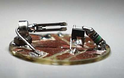
to one of the prongs and then electro-chemically etched to form a sharp tip (fig. 10a).
The preparation of metallic tip for scanning probes is well described in the literature
[20, 21, 22, 23], and in ref. [24] specially the etching of the thin wires used for the tuning
fork tips. For the attachment of the tip it is very important to disturb the symmetry of
the tuning fork as little as possible (sec. 2.3). The metal wire has a diameter of only 15µm
to minimize the additional weight on one prong. A small drop of glue on the other prong
can help to compensate for the additional mass. The wire is either connected with one of
the tuning fork electrodes causing an additional mass of about 1.5 µg, or is is separately
contacted causing an additional weight of up to 50 µg. In the latter case the metal wire
loop causes also an additional spring and damping for the one prong. To keep the wire loop
as short as possible it is attached to a pillar mounted closely to the end of the tuning fork
1
All quantitative data are related to the type shown in figure 1
−12
10
1
10
−13
10
−13
10
0
10
motion (m/sqrt(Hz))
current (A/sqrt(Hz))
charge (e/sqrt(Hz))
−14
10
−14
10
300K
−1
10
−15
10
−15
10
−2
10 1K
−16
10
−16
10
−3
10
32.5 32.55 32.6 32.65 32.7 32.75 32.8 32.85 32.9 32.95 33
frequency (kHz)
Figure 9: The thermal motion of a tuning fork at room temperature (300K) and at 1K. The motion
is converted into a charge via the piezo-electro-mechanical coupling constant α and into a current by
multiplying the charge with the frequency.10
c 2005 Nanonis GmbH, Switzerland, www.nanonis.com, info@nanonis.com
°
Figure 10: Quartz tuning fork sensors for the dynamic force detection. A thin metal wire is attached to
one prong and etched or cut to form a sharp tip (a). The tip is separately contacted to a current to voltage
converter (b) or to a field effect transistor acting as a low input capacitance preamplifier (c). The sensor
plate is mounted on the puck of the xy-table with six screws which also serve for the electrical contacts
(c).
prong (fig. 10b). Tuning fork sensors with separately contacted tip show quality factors
of about 50’000 in vacuum at 4.2K
With a separately contacted tip it is comfortable to perform tunneling or capacitance
measurements. For the small signals as they occur in capacitance measurements and
in Kelvin Probe Microscopy, a Field Effect Transistor (FET) that can be mounted very
closely to the tip is advantageous (sec. 3.3). The FET has to be mounted parallel to the
magnetic field to minimize its effects on the electron gas of the FET. Within this work,
only the configuration where the tip oscillates perpendicular to the sample was tried out,
but also the shear force configuration, where the tip oscillates parallel to the sample is
well established [7].
3.2 The Phase Locked Loop
The frequency shift of the tuning fork is much smaller than that of traditional cantilevers
when the tip interacts with the sample because the spring constant is much higher. This
demands for a frequency demodulation [25] with high resolution and stability. Since
the tuning fork resonance is at a quite low frequency (33kHz), digital signal processing
(DSP) can be applied. This is of great advantage because no analog devices can have a
relative accuracy of 10−9 or better. As shown in figure 4 the phase between the excitation
signal and the current through the fork as a function of the frequency is very steep at
the resonance (about 180 degree/Hz). This allows to detect any shifts in the resonancec 2005 Nanonis GmbH, Switzerland, www.nanonis.com, info@nanonis.com
° 11
frequency very sensitively. With a controller the excitation frequency is then automatically
adjusted to maintain the phase at the value of the resonance. This is the idea of the
PLL and is schematically shown in figure 11. This PLL is put together with standard
laboratory equipment and special software for the integration and automation. This has
the advantage that all the parameters like the detection bandwidth and PI parameters
can easily and transparently be adjusted.
The deviation of the phase is detected with a digital two channel lock-in amplifier (SRS
830) which is synchronized by a digital signal from the frequency generator. The lock-in
amplifier generates two orthogonal sinus signals as reference for the two channels. The
phase of this reference signals with respect to the external synchronization signal can be
shifted by an arbitrary value and is adjusted to have the x-reference signal in phase with
the signal of the tuning fork at the resonance. Ideally this phase shift would be zero (fig. 3)
but the current-to-voltage converters and the long coax cables cause an additional phase
shift. The output of the y-channel which indicates any deviation from the resonance, is
fed into a PI-controller to control the frequency to the resonance.
The frequency generator (Yokogawa FG300) employs the Direct Data Synthesis (DDS)
and has a phase register of 48bit and a clock rate of 40MHz. The span of the frequency
modulation range is typically configured to be 100mHz/V and the resolution for the fre-
quency shift is then about 100µHz. For very sensitive force detection the parameters can
be adjusted to achieve resolutions of the order of 1µHz. However, the stability of the refer-
ence frequency is specified to be 100µHz/o C and for the ultimate frequency shift detection
an external reference frequency with a temperature controlled quartz oscillator (OCXO)
or an atomic clock should be employed.
As an additional feature the oscillation amplitude of the tuning fork is detected with
the x-channel of the lock-in amplifier and the output signal is kept constant by a second
feedback loop which controls the amplitude of the excitation signal. This simplifies the
interpretation of the different recorded signals, since the mechanical oscillation amplitude
of the tuning fork can be assumed to be constant. Second, the transients are avoided that
occur in response to a sudden change in the damping and could last up to seconds for high
quality factors.
The PLL provides two signals that indicate the frequency shift and the excitation
amplitude. Both signals can be used to control the probe sample distance by the z-
feedback controller.
The power dissipated in the tuning fork is the product of the current and the voltage
multiplied by the cosine of the phase angle between the two signals. The phase angle is zero
Yokogawa Stanford
FG320 I-U SR 830 LP
π
DCO
LP
PLL ∆φ
PID amplitude
PID phase
Figure 11: A phase locked loop is employed to measure the frequency shift of the tuning fork. The
driving signal is generated by an digital function generator employing the direct data synthesis method
(DDS). The motion of the tuning fork is detected with a current to voltage amplifier and analyzed with a
digital two channel Lock-in amplifier. Its output signals indicate the mechanical amplitude and the phase
shift, which is used to control the frequency to the resonance. The mechanical amplitude is kept fix by
controlling the amplitude of the excitation signal of the function generator.12 c 2005 Nanonis GmbH, Switzerland, www.nanonis.com, info@nanonis.com
°
on the resonance and is locked by the PLL. The current is kept constant by the amplitude
controller and therefore the amplitude of the excitation signal is a direct measure for the
power dissipation. Any additional damping caused by probe sample interactions can be
detected very sensitively in this manner. Additional power dissipations of the order of
1fW have been detected. This corresponds to an energy loss of 0.2eV per cycle of the
tuning fork with a typical oscillation energy of the order of 105 eV (for 1nm amplitude).
3.3 The Low Temperature Preamplifier
In both, scanning capacitance and in Kelvin probe microscopy, very small amounts of
charges are induced on the tip. This charge elevates the potential of the tip depending on
the capacitance to the rest of the world. When the tip is connected via a coax cable to
a current-to-voltage converter then the cable capacitance is of the order of 100 - 400pF
depending of the length of the cable. The current-to-voltage converter detects the small
rise in voltage and compensates it by letting the current flow over the feedback resistor.
Only a small fraction of about 1% of the charge that is induced on the tip is brought
onto the gate of the first input transistor of the operational amplifier which has typical
input capacitances of the order of 1pF. The rest of the charge is used to fill the cable
capacitance. To overcome this problem it is desirable to have the preamplifier as close
to the experiment as possible eliminating the need of propagating very small signals over
long coax cables. The low temperatures, the high magnetic fields, the limited space and
the low cooling power are not forming the ideal environment for a preamplifier. However,
GaAs-Field-Effect-Transistors (FETs) work even at low temperatures and when mounted
parallel to the magnetic field, it is possible to operate them even at 10 Tesla. The power
consumption can be reduced to reasonably low values but at the expense of the signal to
noise ratio.
In figure 10c a tuning fork sensor with a GaAs FET connected to the tip is shown.
For the detection of the tuning fork itself also a cryo-preamplifier can be used if very low
oscillation amplitudes are desired.
Figure 12 shows the circuit used to drive the preamplifier. The conductivity of the
channel is measured with a current-to-voltage converter keeping the source-drain voltage
USD fixed. Compared to the established source follower circuit, this has the advantage
that the FET can also be operated in the ohmic regime and thus allowing an operation
Utip UGS USD UID
OPA111
+
cold part -
1µF 100kΩ
1kΩ
S D
G FET
10MΩ
tip
Figure 12: The low temperature preamplifier allows to detect small signals very close to the experiment
providing a small input capacitance. The conductance of the channel is measured with a current-to-voltage
converter keeping the Source-Drain voltage fixed and thus allowing an operation at much lower dissipation
power.c 2005 Nanonis GmbH, Switzerland, www.nanonis.com, info@nanonis.com
° 13
with smaller dissipation power. The circuit is powered by batteries and its potential Utip
relative to common ground can be externally defined within ±100V. The output signal is
optically coupled out allowing a completely isolated detection circuit. The whole circuit
and with it the tip can also be modulated with frequencies up to 100kHz without affecting
the output signal except for the capacitive coupling of the tip to its surrounding.
The working point of the FET can be adjusted by the Gate-Source voltage UGS and the
Source-Drain voltage USD . To account for the changing properties of the FET with varying
temperature and magnetic field, the characteristics can be measured in situ allowing the
optimum operation point to be found by giving an additional condition like the maximum
power dissipation or the minimum signal to noise ratio.
The dc-current through the channel of the FET flows over the 1kΩ resistor, and the
small ac-current in addition to the dc-current is taken by the current-to-voltage converter.
The voltage UID has to be adjusted so that no dc-current will cause the current to voltage
converter to come into overload.
The application of the FET as a preamplifier close to the tip allows to detect very
small signals. This is especially advantageous for the Kelvin probe experiments where any
small signal has to be nulled by a bias voltage between the tip and sample. The calibration
and the stability of the amplifier is not important for this application. However, for the
scanning capacitance microscopy the small variations of the tip-sample capacitance have
to be detected in a large background signal from stray capacitances. In this case the gain
of the amplifier has to be stabilized with an accuracy better than 10−4 − 10−6 .
References
[1] J. Rychen. Combined Low-Temperature Scanning Probe Microscopy and Magneto-
Transport Experiments for the Local Investigation of Mesoscopic Systems. PhD thesis,
Swiss Federal Institute of Technology ETH, 2001.
[2] P. Günther, U. Ch. Fischer, and K. Dransfeld. Scanning near-field acoustic mi-
croscopy. Applied Physics B, 48:89–92, 1989.
[3] K. Karrai and Robert Grober. Piezoelectric tip-sample distance control for near field
optical microscopes. Appl. Phys. Lett., 66(14):1842–1844, April 1995.
[4] A. G. Ruiter, J. A. Veerman, K. O. van der Werf, and N. F. van Hulst. Dynamic
behavior of tuning fork shear-force feedback. Appl. Phys. Lett., 71(1):28–30, July
1997.
[5] A. G. T. Ruiter, J. A. Veerman K. O. van der Werf, M. F. Garcia-Parajo, W. H. J.
Rensen, and N. F. van Hulst. Tuning fork shear-force feedback. Ultramicroscopy,
71:149–157, 1998.
[6] W. A. Atia and C. C. Davis. A phase-locked shear-force microscope for distance
regulation in near-field optical microscopy. Appl. Phys. Lett., 70(4):405–407, January
1997.
[7] K. Karrai and I. Tiemann. Interfacial shear force microscopy. Phys. Rev. B,
62(19):13174–13181, November 2000.
[8] H. Edwards, L. Taylor, W. Ducncan, and A. J. Melmed. Fast, high-resolution atomic
force microscopy using a quartz tuning fork as actuator and sensor. J. Appl. Phys.,
82(3):980–984, August 1997.14 c 2005 Nanonis GmbH, Switzerland, www.nanonis.com, info@nanonis.com
°
[9] M. Todorovic and S. Schultz. Magnetic force microscopy using nonoptical piezoelectric
quartz tuning fork detection design with applications to magnetic recording studies.
J. Appl. Phys., 83(11):6229–6231, June 1998.
[10] W. H. J. Rensen adn N. F. van Hulst. Atomic steps with tuning fork based noncontact
atomic force microscopy. Appl. Phys. Lett., 75(11):1640–1642, September 1999.
[11] J. Rychen, T. Ihn, P. Studerus, A. Herrmann, K. Ensslin, H. J. Hug, P. J. A. van
Schendel, and H. J. Güntherodt. Force-distance studies with piezoelectric tuning
forks below 4.2k. Appl. Surf. Sci., 157(4):290–294, April 2000.
[12] J. Rychen, T. Ihn, P. Studerus, A. Herrmann, and K. Ensslin. A low-temperature
dynamic mode scanning force microscope operating in high magnetic fields. Rev. Sci.
Instr., 70(6):2765–2768, June 1999.
[13] J. Rychen, T. Ihn, P. Studerus, A. Herrmann, K. Ensslin, H. J. Hug, P. J. A. van
Schendel, and H. J. Güntherodt. Operation characteristics of piezoelectric quartz
tuning forks in high magnetic fileds at liquid helium temperatures. Rev. Sci. Instr.,
71(3), March 2000.
[14] F. J. Giessibl. High-speed force sensor for force microscopy and profilometry utilizing
a quartz tuning fork. Appl. Phys. Lett., 73(26):3956–3958, December 1998.
[15] A. Arnau, T. Sogorb, and Y. Jiménez. A continous motional series resonant frequency
monitoring circuit and a new method of determining butterworth-van dyke parame-
ters of a quartz crystal microbalance in fluid media. Rev. Sci. Instr., 71(6):2563–2571,
June 2000.
[16] Yoshiro Tomikawa, H. Miura, and S. B. Dong. Analysis of electrical equivalent circuit
elements of piezo tuning forks by the finite element method. IEEE transactions on
sonics and ultrasonics, SU-25(4):206–212, July 1978.
[17] T. R. Albrecht, P. Grütter, D. Horne, and D. Rugar. Frequency modulation detection
using high-q cantilevers for enhanced force microscope sensitivity. J. Appl. Phys.,
69(2):668–673, January 1991.
[18] Robert D. Grober, Jason Acimovic, Jim Schuck, Dan Hessman, Peter J. Kindelmann,
Joao Mespanha, A. Stephen Morse, Khaled Karrai, Ingo Tiemann, and Stephan
Manus. Fundamental limits to force detection using quartz tuning forks. Rev. Sci.
Instr., 71(7):2776–2780, July 2000.
[19] Christian Steiner. Resonanzverhalten von Quartz-Stimmgabeln. Diplomarbeit, Insti-
tut für Fetskörperphysik, ETH Zürich, Prof. Dr. K. Ensslin, 1998.
[20] A. H. Sorensen, U. Hvid, M. W. Mortensen, and K. A. Morch. Preparation of
platin/iridium scanning probe microscopy tips. Rev. Sci. Instr., 70(7):3059–3067,
July 1999.
[21] I. H. Musselman and P. E. Russell. Platin/iridium tips with controlled geometry for
scanning tunneling microscopy. J. Vac. Sci. Technol. A, 8(4):3558–3562, July 1990.
[22] L. A. Nagahara, T. Thundat, and S. M. Lindsay. Preparation and characterization
of STM tips for electrochemical studies. Rev. Sci. Instr., 60(10):3128–3130, October
1989.c 2005 Nanonis GmbH, Switzerland, www.nanonis.com, info@nanonis.com
° 15
[23] J. P. Ibe, P. P. Bey, S. S. Barndow, R. A. Brizzolara, N. A. Burnham, D. P. DiLella,
K. P. Lee, C. R. K. Marrian, and R. J. Colton. On the electrochemical etching of
tips for scanning tunneling microscopy. J. Vac. Sci. Technol. A, 8(4):3570–3575, July
1990.
[24] Peter Vorburger. Construction of a scanning force microscope and force-distance mea-
suremements on gold and graphite surfaces. Diplomarbeit, Institut für Fetskörper-
physik, ETH Zürich, Prof. Dr. K. Ensslin, 1999.
[25] U. Dürig, H. R. Steinauer, and N. Blanc. Dynamic force microscopy by means of the
phase-controlled oscillator method. J. Appl. Phys., 82(8):3641–3651, October 1997.You can also read