Weather-Aware Long-Range Traffic Forecast Using Multi-Module Deep Neural Network - MDPI
←
→
Page content transcription
If your browser does not render page correctly, please read the page content below
applied
           sciences
Article
Weather-Aware Long-Range Traffic Forecast Using
Multi-Module Deep Neural Network
Seungyo Ryu, Dongseung Kim and Joongheon Kim *
 School of Electrical Engineering, Korea University, Seoul 02841, Korea; gpgun@korea.ac.kr (S.R.);
 dkimku@korea.ac.kr (D.K.)
 * Correspondence: joongheon@korea.ac.kr; Tel.: +82-2-3290-3223

 Received: 9 February 2020; Accepted: 9 March 2020; Published: 12 March 2020

 Abstract: This study proposes a novel multi-module deep neural network framework which aims
 at improving intelligent long-term traffic forecasting. Following our previous system, the internal
 architecture of the new system adds deep learning modules that enable data separation during
 computation. Thus, prediction becomes more accurate in many sections of the road network
 and gives dependable results even under possible changes in weather conditions during driving.
 The performance of the framework is then evaluated for different cases, which include all plausible
 cases of driving, i.e., regular days, holidays, and days involving severe weather conditions. Compared
 with other traffic predicting systems that employ the convolutional neural networks, k-nearest
 neighbor algorithm, and the time series model, it is concluded that the system proposed herein
 achieves better performance and helps drivers schedule their trips well in advance.

 Keywords: traffic forecasting; deep learning; neural network; transportation network; weather
 aware prediction

1. Introduction
      The intelligent transport system (ITS) is currently being developed for the road transport
network, and the latest information and communication technology are being worked with. Many
ITS applications, such as traffic control, emergency detection, parking guidance, etc., have extensively
incorporated deep learning, and they showed significant performance improvement [1–3]. This study
reports a novel design of an intelligent traffic forecasting system using deep learning, applied alongside
ITS for efficient driving and urban planning.
      Many studies have used deep learning algorithms for traffic prediction. Some research studies
have considered exploiting neural networks for better analysis of the spatio-temporal correlation of
traffic data. The authors of [4] propose a short-term traffic forecast model using a two-dimensional
long short-term memory (LSTM) network. In [5], the authors use a convolutional neural network
(CNN) by converting traffic data from multiple road sections into 2D images. In [6,7], the authors
adopt Google DeepMind’s WaveNet network and a hierarchical temporal memory model, respectively.
      Research has been conducted for predicting traffic behavior in unusual traffic conditions. In [8],
the authors propose a traffic prediction method based on multi-task learning. They classify traffic
data based on traffic situations and construct situation-aware prediction models. The authors of [9]
suggest a pattern sensitive network with adversarial training. They train a joint distribution model to
improve prediction accuracy under unusual traffic conditions. In [10], the authors adopt a regularized
loss function to balance the predictions of light and heavy traffic conditions.
      Some studies have addressed more interesting factors affecting traffic behavior. In [11], the authors
introduce a rainfall factor into the deep belief network (DBN) and LSTM to predict urban traffic flow.
The authors of [12] combine the flow-based and weather-based traffic model with a DBN, and the

Appl. Sci. 2020, 10, 1938; doi:10.3390/app10061938                               www.mdpi.com/journal/applsci
Appl. Sci. 2020, 10, 1938                                                                            2 of 15

authors of [13] propose a long-term speed prediction method based on LSTM. They analyze the
correlation between the historical parameters of drivers, vehicles, roads, and traffic.
      Research on other data-driven prediction models is still ongoing. In [14], the authors introduce an
iterative k-nearest neighbor predictor for long-term traffic forecasting. The authors of [15,16] propose
k-nearest neighbor traffic prediction models that adopt advanced similarity measures and dynamic
parameter tuning, respectively, and the authors of [17] propose a short-term traffic prediction method
based on an adaptive multi-kernel support vector machine.
      Other researches continue to improve time-series based prediction [18]. Authors of [19] proposed
a traffic prediction scheme using both historical and real-time data. They identified traffic situation with
bayesian network and fused auto-regressive integrated moving average and periodical moving average
model with neural networks. Authors of [20]proposed a long-term traffic forecasting model based
on functional nonparametric regression. They adopted an autocorrelation analysis and a functional
principal component analysis for better accuracy.
      This study proposes a new traffic forecasting model using a multi-module deep neural network
(DNN) framework, called the time and weather aware DNN (TW-DNN). This system is developed
based on our previous design [21], to generate more reliable and complete long-range traffic data.
The framework contains two blocks of neural network modules. The first block extracts various
features from the input, and the second block fuses the features to obtain a traffic prediction output.
Large amounts of data such as weather forecast data, road network information, and traffic speed and
flow data are collected to train the system. The experiments are conducted focusing on multiple traffic
situations, including rush hours, holidays, and heavy rains, and the performance is compared with
that of different but equally capable systems.
      The remainder of this paper is organized as follows. Section 2 introduces the fundamentals
and characteristics of traffic flows. Section 3 presents the proposed intelligent traffic forecasting
using multi-module DNNs.            Section 4 verifies the proposed algorithm via data-intensive
measurement-data-based performance evaluation results. Finally, Section 5 concludes this study
and presents future research approaches.

2. Fundamentals and Characteristics of Traffic Flow
      Because road traffic is determined by the flow of cars, the prediction system should reflect the
information properly. Let f ( x, t) be the traffic flow at the t-th time interval and the x-th location.
The traffic flow consists of three components; speed v( x, t), flow q( x, t), and density d( x, t). They
satisfy the following relationship:
                                                       q( x, t)
                                            d( x, t) =          .                                     (1)
                                                       v( x, t)
    Taking the changes of time and space into account, the traffic flow should meet the following
conservation equation. g( x, t) below denotes the entering flow of the x-th location at t:

                                       ∂q( x, t) ∂d( x, t)
                                                +          = g( x, t),                                  (2)
                                         ∂x        ∂t
   Although they can be computed and used in real life, traffic predictions and simulations may not
make satisfactorily predictions for the following reasons.

•     On the real road, traffic flow can also be affected by non-traffic factors. For example, the traffic
      flow during heavy rain could exhibit unusual speed and density compared to a regular traffic flow.
      In [12], the authors verified the correlations between traffic flow and weather factors, including
      temperature, wind speed, and rainfall. Furthermore, authors of [22] examined that daily weather
      conditions also affected the daily traffic flow.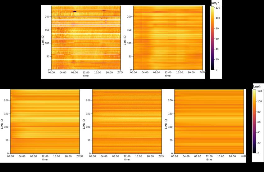
Appl. Sci. 2020, 10, 1938                                                                                            3 of 15

•         Congested traffic shows a different behavior to regular traffic. Authors of [8,10] proposed traffic
          predictions to cope with heavy traffic situations. Day of the week and the time of the day help
          forecast congestion since it usually happens at rush hours and holidays.
•         The actual time and location interval typically do not match those of the numerical model.
          The authors of [23] presented the constraints of time and location intervals to verify the behavior
          of the model. However, the traffic data of some highways do not satisfy those constraints because
          of an insufficient number of installed sensors.

3. New Traffic Forecasting Model Using Multi-Module Deep Neural Networks
     The TW-DNN, which precisely forecasts the speeds of highway networks, is introduced in this
section. Before describing the system, we first introduce the major variables that will be used, as well
as their formats. Traffic data consists of data regarding the speeds and single-lane flows of each
predefined road section (i.e., links), and time. The set of links constructs the highway graph, where
edges and vertices correspond to links and the intersections, respectively. The specific information of a
link such as the number of lanes, length, highway route number, direction, and link shift (the distance
of the current link from the origin of the highway) is stored in the corresponding edge. Because traffic
varies with time, the temporal information such as the date, time, and holiday information is included.
In addition, weather data is included; from these, we consider hourly weather as well as daily weather
information. The hourly weather information represents the local weather of the link, whereas daily
weather covers the weather of nine major cities of South Korea, measured and forecasted by the Korea
Meteorological Administration [24]. Although hourly weather is not available, we estimate it by linear
interpolation. Now, the traffic forecasting system updates the weather every hour. Table 1 shows an
example of inputs for one link. Date, time, and weather data are renewed at the corresponding update
time. All numerical data are normalized to be within [0, 1.0].

                            Table 1. Examples of input data used in our traffic forecasting system.

    Data Class                       Data Subclass               Example #1          Example #2          Example #3
                                     Route number                10                  10                  10
    Link information
                                     Route direction             To East             To East             To East
                                     Linkshift                   50 km               50 km               50 km
                                     Date & time information     2016-9-23 23:55     2016-9-24 0:00      2016-9-24 0:05
    Date & time                      Day of the year             267                 268                 268
                                     Day of the week             Wednesday           Thursday            Thursday
                                     Holiday                     No                  No                  No
                                     Avg. temperature            21.3   ◦C           16.2   ◦C           16.2 ◦ C
    Hourly weather                   Avg. windspeed              2.5 m/s             8.1 m/s             8.1 m/s
                                     Rainfall                    No, 0 mm            Yes, 5 mm           Yes, 5 mm
                                     Snowfall                    No, 0 mm            No, 0 mm            No, 0 mm
                                     Min/Max temperature         16.3 ◦ C/26.8 ◦ C   16.4 ◦ C/28.0 ◦ C   16.4 ◦ C/28.0 ◦ C
    Daily weather of city #1
                                     Cloudiness                  Light               Heavy               Heavy
                                     Rainfall/Snowfall           No/No               Yes/No              Yes/No
    ...                              ...                         ...                 ...                 ...
    Daily weather of city #9         ...                         ...                 ...                 ...

     TW-DNN forecasts all traffic values for a given time range [tstart , tend ] with a resolution of a time
interval (or window) ∆t. As shown in Figure 1, there are two parts functioning together depending on
the prediction periods, as explained below.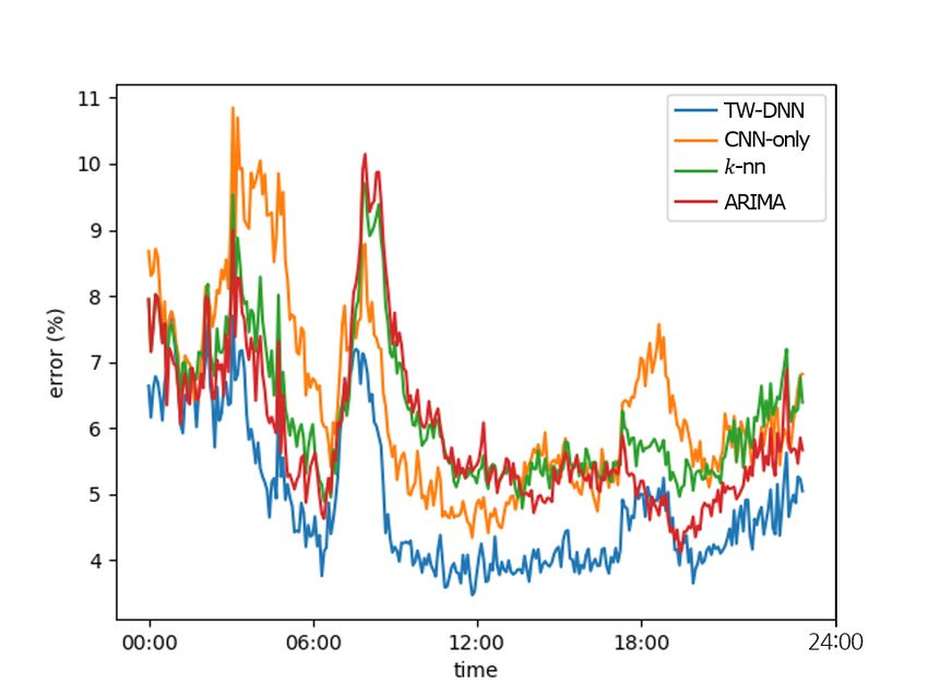
Appl. Sci. 2020, 10, 1938                                                                                4 of 15

1.    The initial traffic predictor predicts the initial speeds and single-lane flows for the first R-time
      intervals, [tstart , tstart + ( R − 1)∆t], using the given link information, date, time, and weather.
2.    The iterative traffic predictor computes the speeds and single-lane flows for each link type (e.g.,
      ordinary link, terminus link, and interchange link) of the following intervals [tstart + R∆t, tend ]
      sequentially, i.e., starting from tstart + R∆t, followed by tstart + ( R + 1)∆t, ..., tend . The predictor
      works in a manner similar to that of a discrete simulation model; it updates the input by the
      current values to proceed to the next time interval.

                     Figure 1. Computing procedure of the TW-DNN. R is a predefined constant.

     Both predictors contain two blocks of neural network modules. Each module serves with the
different input data classes, i.e., traffic data, link information, date, time, and weather. The neural
network with multiple modules has the following characteristics [25].

•     Because the number of input features is reduced and simplified, the neural network can be
      easily optimized.
•     By assigning each input feature to the proper network architecture, prior knowledge of the data
      can be well integrated into the predictor.

     To find out the optimal network architecture of predictor, 1% of training dataset is uniformly
sampled as a validation set. The validation set is not used for training and testing. It helps to select the
best predictor among the group of the predictor with randomly designed network architecture.

3.1. Initial Traffic Predictor
     Figure 2 shows the structure of the initial traffic predictor containing two blocks inside the hidden
layers. In the first block, DNN modules extract hidden features from the input data through fully
connected layers. The CNN module (marked as 1D CNN) performs one-dimensional convolutions
parallel to the DNNs, to obtain features of the daily weather of each region. The second block of DNN
combines individual features before generating the desired traffic data. The output layer predicts
the speed and single-lane flow, using a sigmoid activation function to produce the output value
Appl. Sci. 2020, 10, 1938                                                                            5 of 15

in the range of [0, 1]. The outputs are then converted at the end to recover the original speed and
single-lane flow.

                                   Figure 2. Structure of the initial traffic predictor.

3.2. Iterative Traffic Predictor
     After the initial predictor performs its operations, the iterative traffic predictor is in charge of
delivering all speeds and single-lane flows, for the time intervals [tstart + R∆t, tend ], in a sequential
manner. When the traffic flow of one time-window is determined, the predictor proceeds to the next
window and accepts a new input. The input consists of date, time, weather, and link information,
as well as the traffic data of the previous window. Notably, the speeds, single-lane flows, and link shifts
(from link information) from previous windows are converted and rearranged as described below:

1.     The multi-lane flows (total flows of all lanes), single-lane densities, and multi-lane densities are
       computed using the speeds and single-lane flows.
2.     The traffic data and link shifts are rearranged in a 2D (two dimensional) array by spatial and
       temporal order. 2D array displays the temporal and spatial correlation of traffic data well. Link
       shifts are used to reflect the distance between links. Figure 3 shows the rearranged 2D array of
       link x whose nearby links are x − 1 and x + 1, respectively.

                              Figure 3. Rearrangement of traffic data into 2D arrays.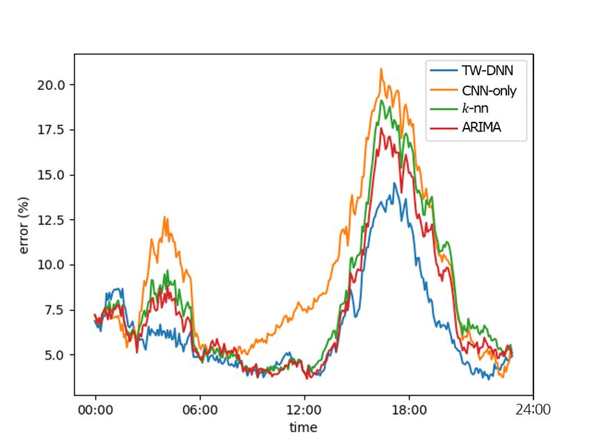
Appl. Sci. 2020, 10, 1938                                                                            6 of 15

      The 2D array is formed to reflect the road network connections; thus, link types are classified into

•     Ordinary link—A middle link connected to a single entrance and exit link,
•     Terminus link—A link connected to local roads at the endpoint of a highway,
•     Interchange link—A link having an additional connection of an on-ramp or off-ramp to a
      joining link.

     Figure 4 shows the structure of the predictor used in the iterative traffic computation. Compared
to the initial traffic predictor, they have an additional module (2D CNN) that accepts the traffic data
obtained in the previous window.

                               Figure 4. Structure of iterative traffic predictor.

      Figure 5 introduces the detailed structure of the 2D CNN that extracts features from the previous
traffic data, considering their spatial and temporal correlation. Inspired from [18], we split the ordinary
convolution having 2 × 2 filters into 2 × 1 and 1 × 2 filters, named Conv2d-space and Conv2d-time,
respectively. They separately process the two parts to prevent interference of the information, resulting
in better prediction performance. The results are combined into the single feature map on the depth
concatenation layer before being fed into the next convolution. At the flatten layer, the feature map is
rearranged into a 1D array, which is suitable for the remaining fully connected layers. Finally, a series
of fully connected layers remaps locally extracted features to yield global representations.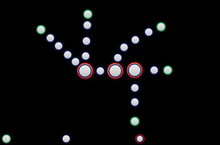
Appl. Sci. 2020, 10, 1938                                                                               7 of 15

                            Figure 5. Structure of 2D CNN accepting previous traffic data.

4. Experimental Results and Discussions

4.1. Experimental Setup
     We tested the developed forecasting system, TW-DNN; the initial setup is described as follows.
For the purpose of comparison, we employed three general traffic prediction models, CNN, k-nearest
neighbor, and autoregressive integrated moving average predictors presented as CNN-only, k-nn,
and ARIMA, respectively [5,14,26]. They were chosen as representatives of the neural network model,
non-neural machine learning model, and time series model, respectively. Figure 6 shows the simplified
view of the TW-DNN, CNN, k-nn, and ARIMA. All models iteratively forecast speeds based on the
previous traffic data. In the prediction, TW-DNN and CNN-only consider many nearby links, whereas
k-nn and ARIMA consider one link at a time. In CNN-only, the prediction results are output after
the data traverses through convolution, pooling, and fully connected layers. Analogous to TW-DNN,
the CNN-only also rearranges supplied input into a 2D array.

                 Figure 6. Simplified view of (a) TW-DNN, (b) CNN-only, (c) k-nn, and (d) ARIMA.

     Meanwhile, k-nn computes the speed by finding the nearest speed values from the
stored dataset that are matched to the previous R windows. It selects a set of k speed
data that minimize the prediction error D (squared error, or the distance), defined as DL =
                                                       2
∑iR=1 vcandidate ( x, t − i∆t) − vtrain L ( x, t − i∆t) , where L represents an index of the stored data. Here,
Appl. Sci. 2020, 10, 1938 8 of 15
vcandidate ( x, t) and vtrain ( x, t) denote the speed values of a candidate and measured data in the training
set, respectively. The prediction output is the average of such k speed values.
ARIMA predicts the speeds with the linear combination of speed data of previous R windows,
as well as the difference and the noisy term of the predicted speed.
Each prediction model was responsible for forecasting speeds for a time interval of 24 h (i.e.,
tend − tstart = 24 h). Three cases of the input were used to represent different road traffic states in the
prediction: a regular day, a holiday, and a day with severe weather. These cases are selected from
year 2016, and weather records for those days are loaded into the TW-DNN. All models are properly
modified to fit our experiments and road network to deliver the best results.
The following are the specific values used in the experiments.
• Prediction time interval ∆t = 5 min
• Historical data used for the current window R = 8, R∆t = 40 min
∆t is equal to the time interval of traffic records. The initial traffic data of all three models were
obtained from the initial traffic predictor of TW-DNN. We used a rectified linear unit and an Adam
optimizer [27] as a default activation function and optimizer, respectively. For k-nn, we empirically
chose k as 5 to yield the best results.
The experiments used a typical highway network surrounding a big city, for which Daegu, South
Korea, was selected. It consists of four bidirectional highways with 241 links, as shown in Figure 7.
The network has five endpoints and 18 interchanges. The traffic data used in the training were obtained
from the Korea Expressway Corporation [28]. This dataset is a collection of traffic data of all nodes
and links recorded every five minutes. Traffic flow and weather data of 2015 were used as a training
dataset, which was preprocessed prior to utilization in the prediction models as follows.
Figure 7. Highway network with city names used in the experiments (the labels represent the name of
the location).
• When the training dataset was extracted, speeds and flows larger than the 98th percentile were
removed as outlier data.
• The time-domain moving averages of the speeds and flows were used instead of the raw data,
to reduce noise. The window size for moving the average of time t was chosen as [t − ∆t, t + ∆t].
• All data were linearly scaled to lie within [0, 1.0].
Experiments were performed using a Linux-based workstation having an Intel i7-7700 CPU with
32 GB RAM and a GPGPU of the Nvidia GeForce GTX 1080. The prediction models were programmedAppl. Sci. 2020, 10, 1938 9 of 15
using scikit-learn, TensorFlow, and pmdarima packages. Prediction errors are expressed using standard
forms such as the mean absolute error (MAE) and mean absolute percentage error (MAPE). They are
computed as shown below:
∑in=1 | Ai − Fi |
MAE , , (3)
n
n
100% A − Fi
MAPE , ×∑ i , (4)
n i =1
Ai
where Ai , Fi , and n denote the real (measured) value, forecast value, and amount of data, respectively.
4.2. Experimental Results
4.2.1. Case I (Regular Day)
Figure 8 plots the MAPE of each prediction model. The errors of CNN-only, k-nn, and ARIMA
are unusually large during dawn and rush hour, respectively. In most cases, TW-DNN produces the
best results, with only a smaller error (by 4% at most), compared to the others.
Figure 8. MAPE error of prediction models for Case I.
Figure 9 shows the predicted speeds of each model in colors; this is called a heatmap. Blue and
yellow represent low and high speeds, respectively, while white only in the real data represents missing
data. Both the link (location) and time are displayed in the vertical and horizontal axes, respectively.
Careful observation of the real data in Figure 9a indicates that speeds are populated between 80 and
120 km/h in general. The real traffic data show two interesting phenomena:
• The speeds at dawn (2:00–5:00) are recorded to be around 80 km/h, while those at daytime
(6:00–18:00) are recorded to be around 100 km/h.
• There is severe congestion (i.e., speed lower than 20 km/h) in some links at around 8:00 and 18:00.
TW-DNN data shows a close match to the real data, while CNN-only, k-nn, and ARIMA data
do not.Appl. Sci. 2020, 10, 1938 10 of 15
Figure 9. Speed figure of (a) real data, (b) TW-DNN, (c) CNN-only, (d) k-nn, and (e) ARIMA for Case I.
4.2.2. Case II (Holiday)
Case II corresponds to the holiday season, during which heavy traffic is present on the roads.
Figure 10 shows the MAPE, where significant errors appear around 12:00. TW-DNN outperforms
others, showing smaller errors by up to 6%, 3%, and 5%, compared to CNN-only, k-nn and ARIMA,
respectively.
Figure 10. MAPE error of prediction models for Case II.
The heatmap of Case II is shown in Figure 11. In real traffic, congestion occurs between 12:00 and
20:00 in some links. TW-DNN detects congestion successfully except in some links. It also forecasts
the regular traffic condition similar to the real data. Although the other models do not detect the
congestion, they somehow only show small error in this case.Appl. Sci. 2020, 10, 1938 11 of 15
Figure 11. Speed figure of (a) real data, (b) TW-DNN, (c) CNN-only, (d) k-nn, and (e) ARIMA for
Case II.
4.2.3. Case III (Severe Weather Day)
Case III covers a day in which the rainfall starts at 2:00 and continues until the end of the day.
TW-DNN shows the least MAPE among the models, as shown in Figure 12, and significant gaps
between TW-DNN and others can be observed around 4:00 and 17:00. The phenomena are better
explained in the speed heatmap.
Figure 12. MAPE error of prediction models for Case III.
The real data show some speed slow-down for the periods of 02:00–05:00 and 15:00–19:00.
TW-DNN predicts the congestion due to the rainfall, especially at dawn and rush hours. However,
CNN-only, k-nn, and ARIMA cannot predict it because they do not consider weather factors at all.Appl. Sci. 2020, 10, 1938 12 of 15
4.3. Summary and Discussion
The overall MAE and MAPE of the prediction models are summarized in Table 2. The bold
numbers show the best prediction errors for each case. TW-DNN has the lowest error in all three cases.
Table 2. Average mean absolute error and mean absolute percentage error of the test cases.
Mean Absolute Error Mean Absolute Percentage Error
TW-DNN CNN-Only k-nn ARIMA TW-DNN CNN-Only k-nn ARIMA
Case I
4.75 6.24 6.07 5.82 4.87 6.40 6.40 5.96
(Regular day)
Case II
7.24 10.05 8.38 9.14 7.68 10.58 9.37 9.59
(Holiday)
Case III
6.01 8.48 7.40 6.86 6.48 9.23 8.07 7.46
(Severe weather day)
How accurately the models forecast the congestion is summarized in Table 3. Congested and
congestion-free are distinguished from the speed of 70 km/h. TW-DNN delivers the best result.
Although heatmaps in Figures 9, 11, and 13 show the close match of prediction between TW-DNN and
actual data, the prediction accuracy does not seem good enough, i.e., TW-DNN predicts lighter and
shorter congestion than actual traffic data.
Figure 13. Speed figure of (a) real data, (b) TW-DNN, (c) CNN-only, (d) k-nn, and (e) ARIMA for
Case III.Appl. Sci. 2020, 10, 1938 13 of 15
Table 3. Accuracy of predicting congestion for the test cases
Congested Link Congestion-Free Link
TW-DNN CNN-Only k-nn ARIMA TW-DNN CNN-Only k-nn ARIMA
Case I
0.0 0.0 0.0 0.0 99.79 99.79 99.78 99.79
(Regular day)
Case II
21.41 0.0 0.0 0.0 96.29 95.92 95.91 95.92
(Holiday)
Case III
42.93 0.0 0.0 0.0 97.59 97.57 97.53 97.71
(Severe weather day)
The novel features of our prediction model are listed to summarize the experimental results.
• Date-, time-, and weather-aware traffic prediction: The real speed data show that time and
weather do indeed affect road traffic. Upon addition of the time and weather modules, TW-DNN
could predict congestion in unusual situations, while the others could not predict the congestion
at all. They were not able to account for the weather and temporal condition.
• Spatial correlation of traffic flow: To reflect the spatial correlation of the traffic flow, TW-DNN
predicts the speeds of the links better, using the traffic information of the surrounding links. k-nn
and ARIMA cannot outperform TW-DNN because it does not have the traffic information of
adjacent links.
• Type of a link: TW-DNN uses different predictors depending on the connection structures of
the links. Meanwhile, CNN-only, k-nn, and ARIMA do not reflect the structural differences of
the highway links. TW-DNN effectively predicted the speed values of interchange links having
ramps, while the others did not.
5. Concluding Remarks and Future Work
In this study, a novel multi-module DNN framework was proposed for intelligent traffic
forecasting. The framework was designed to improve our previous system, realize a long prediction
period range, and obtain a weather-aware traffic prediction using short-term and long-term weather
forecast data. Experimental results proved that our framework exhibits an efficient performance
on forecasting traffic for all kinds of driving situations such as regular days, holidays, and days of
severe weather.
More work would be needed to improve the computation speed and accommodate the live
traffic-related information encountered during driving. The system may need a new module in charge
of interacting with the current ones to dynamically reflect such real-time traffic data.
Author Contributions: S.R. and D.K. were the main researchers who initiated and organized the research work
reported in the paper; S.R. and J.K. were responsible for building the final TW-DNN to improve its functions
and performance. All authors have read and agreed to the published version of the manuscript.
Funding: This research was supported by the Basic Science Research Program through the National Research
Foundation of Korea (NRF) funded by the Ministry of Education (grant number: NRF-2018R1D1A1B07046195)
and also by NRF-Korea (grant number: 2019R1A2C4070663).
Conflicts of Interest: The authors declare no conflicts of interest.
References
1. Shengdong, M.; Zhengxian, X.; Yixiang, T. Intelligent Traffic Control System Based on Cloud Computing
and Big Data Mining. IEEE Trans. Ind. Inf. 2019, 15, 6583–6592.
2. Zhu, L.; Guo, F.; Krishnan, R.; Polak, J.W. A Deep Learning Approach for Traffic Incident Detection in Urban
Networks. In Proceedings of the 2018 21st International Conference on Intelligent Transportation Systems
(ITSC), Maui, HI, USA, 4–7 November 2018; pp. 1011–1016.Appl. Sci. 2020, 10, 1938 14 of 15
3. Barbancho, J.; Ropero, J.; Luque, J.; Caraballo, A.; León, C. Social Parking: Applying the Citizens as Sensors
Paradigm to Parking Guidance and Information. Sustainability 2019, 11, 6549, doi:10.3390/su11236549.
4. Zhao, Z.; Chen, W.; Wu, X.; Chen, P.C.Y.; Liu, J. LSTM Network: A Deep Learning Approach for Short-Term
Traffic Forecast. IET Intell. Transp. Syst. 2017, 11, 68–75.
5. Ma, X.; Dai, Z.; He, Z.; Ma, J.; Wang, Y.; Wang, Y. Learning Traffic as Images: A Deep Convolutional
Neural Network for Large-Scale Transportation Network Speed Prediction. Sensors 2017, 17, 818,
doi:10.3390/s17040818.
6. Impedovo, D.; Dentamaro, V.; Pirlo, G.; Sarcinella, L. TrafficWave: Generative Deep Learning Architecture
for Vehicular Traffic Flow Prediction. Appl. Sci. 2019, 9, 5504, doi:10.3390/app9245504.
7. Mackenzie, J.; Roddick, J.F.; Zito, R. An Evaluation of HTM and LSTM for Short-Term Arterial Traffic Flow
Prediction. IEEE Trans. Intell. Transp. Syst. 2019, 20, 1847–1857.
8. Deng, D.; Shahabi, C.; Demiryurek, U.; Zhu, L. Situation Aware Multi-task Learning for Traffic Prediction. In
Proceedings of the 2017 IEEE International Conference on Data Mining (ICDM), New Orleans, LA, USA,
18–21 November 2017; pp. 81–90.
9. Lin, Y.; Dai, X.; Li, L.; Wang, F.-Y. Pattern Sensitive Prediction of Traffic Flow Based on Generative Adversarial
Framework. IEEE Trans. Intell. Transp. Syst. 2019, 20, 2395–2400.
10. Fouladgar, M.; Parchami, M.; Elmasri, R.; Ghaderi, A. Scalable Deep Traffic Flow Neural Networks for Urban
Traffic Congestion Prediction. In Proceedings of the 2017 IEEE International Joint Conference on Neural
Networks (IJCNN), Anchorage, AK, USA, 14–19 May 2017; pp. 2251–2258.
11. Jia, Y.; Wu, J.; Xu, M. Traffic Flow Prediction with Rainfall Impact Using a Deep Learning Method. J. Adv.
Transp. 2017, 2017, 1–10, doi:10.1155/2017/6575947.
12. Koesdwiady, A.; Soua, R.; Karray, F. Improving Traffic Flow Prediction With Weather Information in
Connected Cars: A Deep Learning Approach. IEEE Trans. Veh. Technol. 2016, 65, 9508–9517.
13. Yufang, L.; Mingnuo, C.; Wanzhong, Z. Investigating Long-Term Vehicle Speed Prediction based on BP-LSTM
Algorithms. IET Intell. Transp. Syst. 2019, 13, 1281–1290.
14. Yu, B.; Song, X.; Guan, F.; Yang, Z.; Yao, B. k-Nearest Neighbor Model for Multiple-Time-Step Prediction of
Short-Term Traffic Condition. J. Transp. Eng. 2016, 142, 04016018.
15. Habtemichael, F.G.; Cetin, M. Short-Term Traffic Flow Rate Forecasting based on Identifying Similar Traffic
Patterns. Transp. Res. Part C Emergy Technol. 2016, 66, 61–78.
16. Sun, B.; Cheng, W.; Goswami, P.; Bai, G. Flow-Aware WPT k-Nearest Neighbours Regression for Short-Term
Traffic Prediction. In Proceedings of the 2017 IEEE Symposium on Computers and Communications (ISCC),
Heraklion, Greece, 3–6 July 2017; pp. 48–53.
17. Feng, X.; Ling, X.; Zheng, H.; Chen, Z.; Xu, Y. Adaptive Multi-Kernel SVM With Spatial–Temporal Correlation
for Short-Term Traffic Flow Prediction. IEEE Trans. Intell. Transp. Syst. 2019, 20, 2001–2013.
18. Mehta, S.; Hajishirzi, H.; Rastegari, M. DiCENet: Dimension-wise Convolutions for Efficient Networks.
arXiv 2019, arXiv:1906.03516.
19. Xie J.; Choi, Y.-K. Hybrid Traffic Prediction Scheme for Intelligent Transportation Systems based on Historical
and Real-Time Data. Int. J. Distr. Sens. Netw. 2017, 13, 1–11.
20. Su, F.; Dong, H.; Jia, L.; Qin, Y.; Tian, Z. Long-Term Forecasting Oriented to Urban Expressway Traffic
Situation. Adv. Mech. Eng. 2016, 8, 1–16
21. Ryu, S.; Kim, D. Intelligent Highway Traffic Forecast Based on Deep Learning and Restructured Road Models.
In Proceedings of the 2019 IEEE 43rd Annual Computer Software and Applications Conference (COMPSAC),
Milwaukee, WI, USA, 15–19 July 2019; pp. 110–114.
22. Cools, M.; Moons, E.; Wets, G. Assessing the Impact of Weather on Traffic Intensity. Wea. Clim. Soc. 2010, 2,
60–68.
23. Messmer, A.; Papageorgiou, M. METANET: A Macroscopic Simulation Program for Motorway Networks.
Traff. Eng. Control 1990, 31, 466–470.
24. Korea Meteorological Administration. Available online: Http://kma.go.kr (accessed on 13 January 2020).
25. Chen, K. Deep and Modular Neural Networks. In Springer Handbook of Computational Intelligence; Kacprzyk, J.,
Pedrycz, W., Eds.; Springer: Berlin/Heidelberg, Germany, 2015; pp. 473–494, ISBN 978-3-662-43505-2.
26. Ahmed, M.S.; Cook, A.R. Analysis of freeway traffic time-series data by using Box–Jenkins techniques.
Transp. Res. Rec. 1979, 722, 1–9.Appl. Sci. 2020, 10, 1938 15 of 15
27. Kingma, D.P.; Ba, J. Adam: A Method for Stochastic Optimization. arXiv 2017, arXiv:1412.6980.
28. Korean Expressway Public Data Portal. Available online: Http://data.ex.co.kr (accessed on 13 January 2020).
© 2020 by the authors. Licensee MDPI, Basel, Switzerland. This article is an open access
article distributed under the terms and conditions of the Creative Commons Attribution
(CC BY) license (http://creativecommons.org/licenses/by/4.0/).You can also read