MATHWORKS MATH MODELING CHALLENGE 2021 - PINE VIEW SCHOOL
←
→
Page content transcription
If your browser does not render page correctly, please read the page content below
MathWorks Math Modeling Challenge 2021
                                                   Pine View School
                             Team # 14525 Osprey, Florida
                                   Coach: Mark Mattia
Students: Uday Goyat, Grace Jiang, Maxim Kasyanenko, Julia Kourelakos, Danny McDonald

                               M3 Challenge Technical Computing Award
                               THIRD PLACE—$1,OOO Team Prize

JUDGES’ COMMENTS
Specifically for Team # 14525 —Submitted at the Close of Technical Computing Contention Judging:
COMMENT 1: This paper stood out for its creative and ambitious use of technical computing. It included a well-implemented
Monte Carlo method for Part 2, which constructed random “schedules” to determine the maximum bandwidth used by a family
over the course of a year. For Part 3, the students utilized ArcGIS software to build a sophisticated model for placing cellular nodes.
They took into account information about road locations, elevation, and conservation land, with final node locations chosen via an
iterative greedy algorithm. While clear at times, a lack of details and missing information about the methods used was a weakness
in the report. Some modeling decisions also lacked justification or were unclear. However, all-in-all, this was a fun report to read,
with a lot of great ideas.

Specifically for Team # 14525 —Submitted at the Close of Technical Computing Triage Judging:
COMMENT 1: Team could have benefitted from captioning the figures accurately. The levels were not readable.
COMMENT 2: The executive summary is well-written with overview of the questions, insight into solution approach, and summary
of results. The team proposed an exponential decay model for Q1 where they predict the cost per unit of bandwidth for the next 10
years for the US. I guess due to lack of data for the UK they were unable to come up with a model. I am particularly happy with the
approach taken to arrive at their result and also pleased with the discussion of the strength and weaknesses of the model. The team
provided several interesting and reasonable assumptions and justifications for Q2. Several graphs that are normally distributed to
represent their model were shown. Graphs were properly labeled and strength and weaknesses discussed. Similar approach is taken
in modeling the problem for Q3 but using the ArcGIS tool. The team also used Python to implement their proposed model.
COMMENT 3: This is a very interesting work. Good job overall.
COMMENT 4: Very well written summary. Each model was developed well, executed, strengths and weaknesses discussed and
justification applied. Sensitivity analysis applied appropriately.
COMMENT 5: Your executive summary was good, but you didn’t state your most fundamental answers, explicitly. In Q1, you
may have desired to consider cost of bandwidth will never be zero. Section 1.6.1 was not required. Please label all tables. In
Q2, I would’ve liked to see multitasking involving your assumption. Overall, your assumptions were strong. You were wise to
acknowledge the dependence of your research on the available literature. This is true for many researchers! Your answer to Q3 was
very creative, though an emphasis on demographic characteristics would’ve strengthened it. Overall, very well written in plain
language. Excellent techniques.

                                                         ***Note: This cover sheet was added by SIAM to identify the winning team
                                                         after judging was completed. Any identifying information other than team #
                                                         on a MathWorks Math Modeling Challenge submission is a rules violation.
                                                         ***Note: This paper underwent a light edit by SIAM staff prior to posting.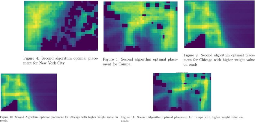
Team 14525 Page 1
Defeating the Digital Divide: Internet Costs, Needs,
and Optimal Planning
Executive Summary
Over the past few years, the internet has become something of a daily necessity: allowing
attendance at school, providing a medium for digital entertainment, allowing a medium
for digital entertainment, revolutionizing the healthcare industry. But not everyone has
access to the internet. There are a number of near-insurmountable challenges surrounding
the availability of the internet.
Internet transit was considered in order to extrapolate the cost per unit of Megabytes per
second of broadband. Internet transit is the service which allows a computer to connect to
an ISP. The data was found for the prices per Mbps of internet transit from 1998 to 2015.
Regression was used to fit an exponential decay into the function. The time was
extrapolated for the next 10 years, and the percentage decrease was determined. We then
used regression software and determined a correlation coefficient R2 to be approximately
0.9879320769, which entails our exponential decay model closely fit the prescribed data set.
For Part 2, we used two Monte Carlo simulations (one in the presence of COVID-19, one
without the presence of COVID-19) to model the maximum daily bandwidth usage of three
different types of households over the course of a year, creating normally distributed ran-
domized schedules for individuals in each household. We found that households use more
bandwidth during COVID than without COVID (most likely due to the need to use one’s
own bandwith for school and work during COVID), and that 99% of all three types of house-
holds’ internet needs could be easily satisfied with 81.5 megabits per second of bandwidth.
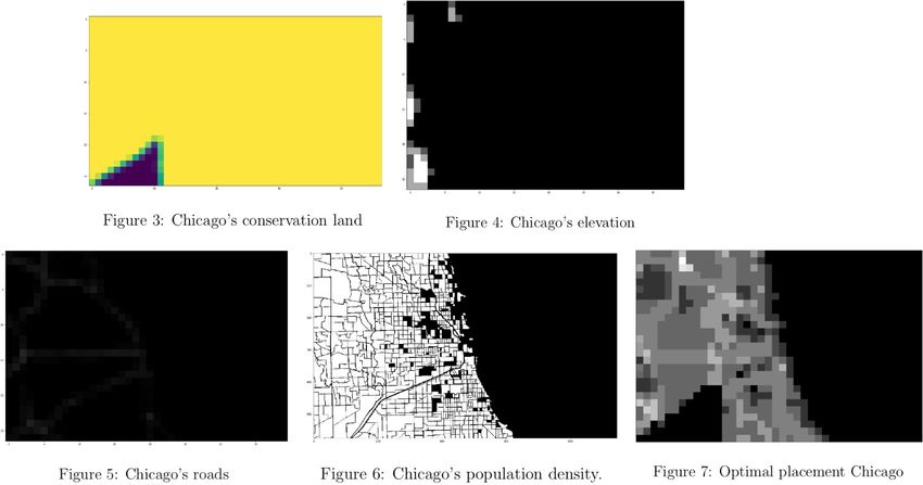
Three cities---Tampa, Chicago, and New York City---were chosen for part 3. ArcGIS (A ge-
ographic information system) was used to extract and then later scrape and scale the 4
different factors: elevation, population density, highways and roads, and conservation land.
Two different algorithms were proposed which relied on different ways of spreading the sig-
nal based on elevation. The roads were more desirable for placement of towers due to high
activity and population. Towers were also desirable to be placed near high population den-
sity. Conservation areas were completely avoided. Finally, sensitivity analysis was done by
assigning each factor a weight (keeping conservation area weight to 0) and changing the
weights to align with different city, rural and suburban settings.
In order to predict the optimal positioning of cellular towers, a Radial Coverage Conver-
gence (RCC) algorithm was devised and employed to greedily eliminate the highest tower
dependency scores in an iterative manner until a certain convergence threshold is met.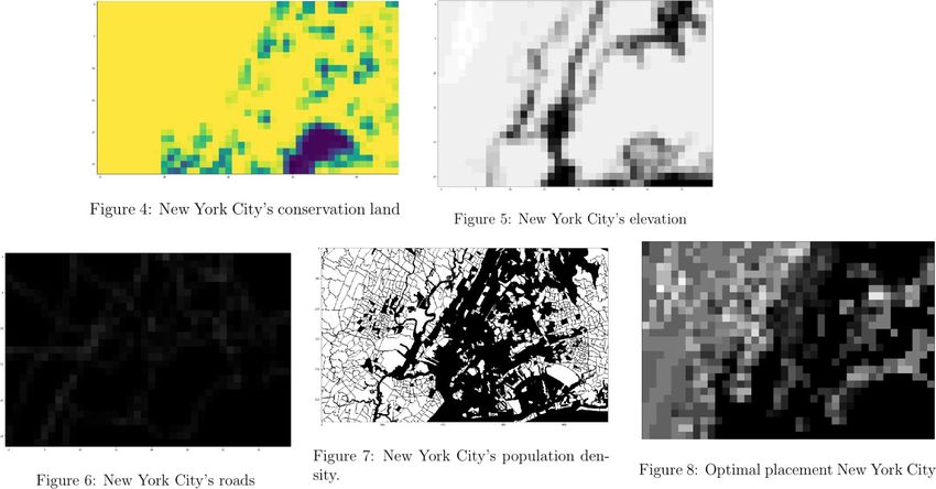
Team 14525                                                                                                        Page 2

Contents
1 The Cost of Connectivity                                                                                                 3
  1.1 Defining the Problem . . . . . . . . . . . . . . . . . . . . . . . . . . . . . .                              .      3
  1.2 Assumptions . . . . . . . . . . . . . . . . . . . . . . . . . . . . . . . . . . .                             .      3
  1.3 Variables Used . . . . . . . . . . . . . . . . . . . . . . . . . . . . . . . . .                              .      3
  1.4 Developing the Model . . . . . . . . . . . . . . . . . . . . . . . . . . . . . .                              .      3
  1.5 Executing the Model . . . . . . . . . . . . . . . . . . . . . . . . . . . . . .                               .      4
  1.6 Results and Discussion . . . . . . . . . . . . . . . . . . . . . . . . . . . . .                              .      5
      1.6.1 Further Validation . . . . . . . . . . . . . . . . . . . . . . . . . . .                                .      5
      1.6.2 Strengths and Weaknesses . . . . . . . . . . . . . . . . . . . . . . .                                  .      5

2 Bit     by Bit                                                                                                            6
  2.1      Defining the Problem . . . . . . . . . . . . . . . . . . . . . . . . . . . . . . .                               6
  2.2      Assumptions . . . . . . . . . . . . . . . . . . . . . . . . . . . . . . . . . . . .                              6
  2.3      Variables Used . . . . . . . . . . . . . . . . . . . . . . . . . . . . . . . . . .                               8
  2.4      Developing the Model . . . . . . . . . . . . . . . . . . . . . . . . . . . . . . .                               8
  2.5      Executing the Model ........................................................................................... 10
           2.5.1 Strengths and Weaknesses .......................................................................12

3 Mobilizing Mobile                                                                                                        12
  3.1 Defining the Problem ...........................................................................................12
  3.2 Assumptions ........................................................................................................ 12
  3.3 Variables Used ......................................................................................................12
  3.4 Developing the Model ..........................................................................................12
  3.5 Executing the Model ............................................................................................13
  3.6 Results and Discussion ....................................................................................... 16
      3.6.1 Sensitivity Analysis ................................................................................... 17
      3.6.2 Strengths and Weaknesses ....................................................................... 17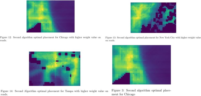
Team 14525                                                                         Page 3

1     The Cost of Connectivity
1.1    Defining the Problem
We were asked to devise a model to predict the cost per unit bandwidth in U.S. dollars per
megabits per second (Mbps) over the next ten years for consumers in both the United States
and the United Kingdom.

1.2    Assumptions
1-1. We can use an exponential model to perform exponential regression on the
     historical bandwidth costs data.

        • Justification: According to Nielsen’s Law, the growth of bandwidth will grow
          exponentially over time [4]. By the law of supply and demand [5], this means
          that the the prices of bandwidth will decrease over time. We will show how this
          decrease is exponential later in Section 1.5.
1-2. The bandwidth price of $0.34 for the U.K. in 2017 will be used to
    extrapolate the U.S. future bandwidth predictions onto the U.K..

        • Justification: This statistic is given by Internet Service Provider Review U.K.
          [6].

1.3    Variables Used

              Symbol           Definition             Units Value
                P          Price of Bandwidth        $/Mbps  ...
                P0     Initial Price of Bandwidth    $/Mbps  ...
                r      Rate of Exponential Decay       ...   ...
                 t   Years Passed Since Initial Year years   ...

1.4    Developing the Model
To create a model predicting the price of bandwidth over the next 10 years, we needed data
describing bandwidth prices in recent history. We were able to locate data concerning the
bandwidth prices in the United States in dollars per Mbps from the years 1998 to 2015 [2].

To obtain an idea of the type of regression model we must employ to solve the problem, we
plotted the raw data for U.S. bandwidth prices over time. This is shown in Figure 1 below.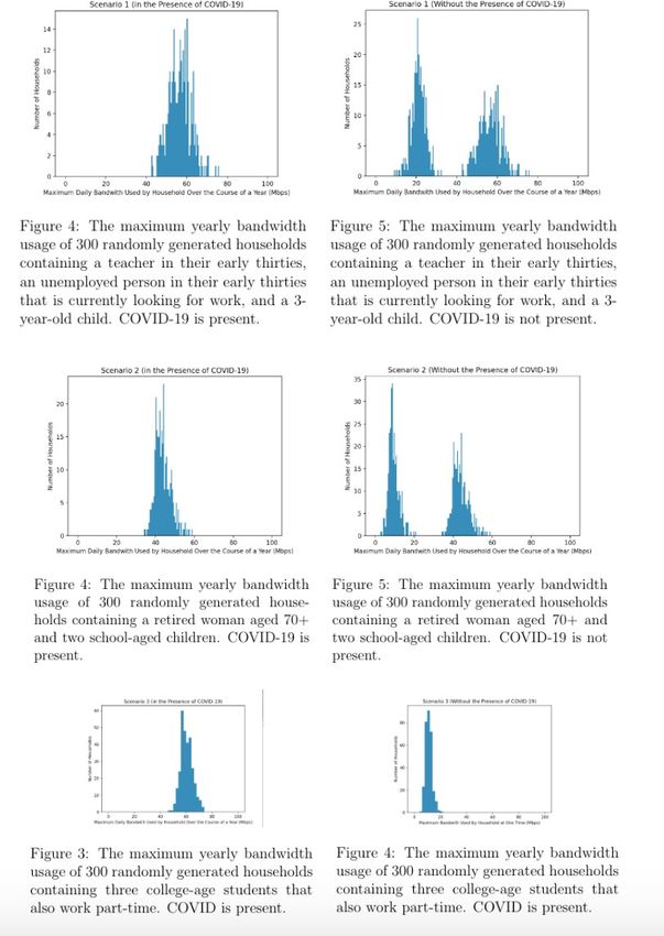
Team 14525                                                                           Page 4

      Figure 1: Graph of raw data of bandwidth prices in the U.S. from 1998 to 2015.

From this graph, we can see that the bandwidth prices from 1998 to 2015 have decreased
in a pattern closely paralleling that of an exponential decay model. We can therefore apply
the following model to predict the bandwidth prices in the U.S. for the next 10 years.

                                        P (t) = P0(rt)

In this model, r represents the rate of decay and must be a value between 0 and 1, P0
represents the initial price of bandwidth, t represents any given year, and P represents the
price of bandwidth at that given year.

1.5    Executing the Model
Utilizing an exponential regression calculator, we were able to obtain a model to fit our data
on bandwidth prices in the U.S. from 1998 to 2015. This model was then plotted alongside
our earlier plot of the raw data. In Figure 2 below, the raw data is the blue line, while the
exponential regression model is the orange line.

          Figure 2: Exponential regression line of bandwidth prices in the U.S.
Team 14525                                                                            Page 5

Unfortunately, we were unable to find data on historical prices of bandwidth in the United
Kingdom. Thus, we were unable to utilize exponential regression to predict the cost in
bandwidth over the next 10 years in the U.K.. However, using the statistic that the average
cost per Mbps of broadband speed in the U.K. was $0.34 in the year 2017 [6], we are able
to extrapolate bandwidth prices in the U.K. for the next 10 years based on predicted
bandwidth prices in the U.S. for 2017 and the next 10 years.

1.6     Results and Discussion
From our exponential regression model of bandwidth prices in the U.S., we were able to
predict the bandwidth prices in the U.S. for the next 10 years. The results of this are shown
below.

1.6.1   Further Validation
One strength of our model lies in its strong coefficient of correlation.

1.6.2   Strengths and Weaknesses
One strength of our model lies in its strong coefficient of correlation. Through utilizing
regression software, we found our R2 coefficient to be approximately 0.9879320769. This
suggests that our particular exponential function that we modeled is positively correlated to
the points we used from the data set. We note, however, the R2 value is solely indicative of
the validity of our Python model that we trained: it is not a measure of the validity of our
prediction.

One weakness of our model comes from our reliability on a small data set. Because we were
unable to find a large data set, we used the MathWorks information sheet [1] and Dr.Peering
[2] to fit an exponential decay model. We then trained a model that was predicated on this
prior data to predict the cost over the next ten years. Since we used a small data set to
train the data, our model is very sensitive to perturbations in the data, i.e., our model would
not give an accurate prediction for the cost of per unit bandwidth over time. However, our
model can be re-trained if given supplemental data, such that it is not sensitive to changes
in the data set.
Team 14525                                                                            Page 6

Another weakness is that our model was not able to provide a prediction for the U.K. over the
next ten years. However, we did find, according to a recent 2017 study [6], that the cost of
broadband per Mbps is approximately $0.34. We suggest a similar regression process for
determining the value, considering 2017 as our base year.

Another weakness lies in our consideration of transit price as a replacement for broadband.
We could not find any data regarding the cost of broadband over time; however, we could find
data on transit price. Because transit price is determined by the internet service provider
(ISP) we note that there is a disparity between the cost of broadband and the transit price;
the ISP charges a high markup price on the broadband in effort to make a profit. We note,
however, that, if given new data for the real broadband price, then we will likely find a
similar regression to our model due to the fact that the broadband price is merely a fraction
of the transit price.

For further research, we suggest extrapolating SEC findings to determine the exact markup
price and provide a better estimate for the cost of broadband per Mbps.

2     Bit by Bit
2.1     Defining the Problem
We were asked to develop an adaptable model that would determine the minimum amount
of required bandwidth that would fulfill three hypothetical households’ total internet needs
90% of the time and 99% of the time.

The hypothetical households are as follows:
    1. Scenario 1: a couple (in which one is actively seeking work and the other is a teacher)
       in their early thirties with a three-year-old child.
    2. Scenario 2: a retired woman in her seventies whose two school-aged grandchildren
       come over twice a week.
    3. Scenario 3: three former M3 Challenge participants sharing an apartment while
       pursuing their undergraduate studies full-time and working part-time.

2.2     Assumptions
2-1. The only three purposes for which individuals in a household use bandwidth
     are work, education, and recreation; individuals can only engage in one of these
     three activities at once.
         • Justification: These are the three most notable uses of the internet and encom-
           pass a wide range of activities.
2-3. The mean amount of time spent in school by a full-time student on a weekday is
     6.64 hours, and the standard deviation is 0.245 hours.
Team 14525 Page 7
• Justification: These statistics for the number of hours in the school day in the
United States were taken from the National Center for Education Statistics
[D6].
2-4. The mean start time for school is 8:03 AM, and the standard deviation is 11
minutes.
• Justification: These are the statistics for the start times of all public middle,
high, and combined schools in the United States according to CDC data
[https://www.cdc.gov/mmwr/preview/mmwrhtml/mm6430a1.htm].
2-5. 42% of all full-time workers in the U.S. work a 40-hour workweek, followed
by 21% who work 50-59 hours/week, 18% who work 60+ hours/week, 11% who
work 41-49 hours/week, and 8% who work fewer than 40 hours/week.
• Justification: These statistics are given by 2013 and 2014 Work and Education
polls [8].
2-6. Individuals engage in four types of recreation: watching cable television,
browsing the web or social media, streaming video, or gaming. Bandwidth used
for these activities is in accordance with FCC statistics.
• Justification: The FCC has comprehensively broken down recreational activi-
ties by bandwidth usage [7].
2-6. The mean amount of time spent at work on a weekday by a part-time employee
is 5.58 hours.
• Justification: This statistic is from the U.S. Bureau of Labor Statistics [D7].
2-6. All individuals within a household are in the same income bracket.
• Justification: Individuals that share a house are most likely either sharing
finances (as in the case of a married couple or a husband and child) or able to
afford to rent/own the same domicile.
2-7. The maximum amount of required bandwidth for hypothetical household 2 will
be on the days the two school-aged grandchildren are over at the retired
woman’s house.
• Justification: The more people there are in the household, the more people
there will be simultaneously on the internet. Thus, more bandwidth will be
required to support internet usage when the grandchildren are at the
grandmother’s house.Team 14525 Page 8
2.3 Variables Used
Symbol Definition Units Value
Iw Individuals Using Bandwidth for Work Individuals ...
Ie Individuals Using Bandwidth for Education Individuals ...
Ir Individuals Using Bandwidth for Recreation Individuals ...
Bw Bandwidth Required for One Individual Working Mbps ...
Be Bandwidth Required for One Individual’s Education Mbps ...
Br Bandwidth Required for One Individual’s Recreation Mbps ...
U Usage of Bandwidth at a Given Moment Mbps ...
2.4 Developing the Model
A household’s bandwidth is the amount of information, in megabits per second (Mbps), that
it can simultaneously send or receive over the internet at any given moment.
Although the amount of bandwidth allotted to each household bandwidth is fixed, usage
of it fluctuates---not only from day to day, but also over the course of each day. Multiple
household members using the internet at the same time will require more bandwidth than
one individual alone; some uses of the internet, such as streaming video, take up more band-
width than other uses of the internet, such as checking one’s email. Thus, a household’s need
for bandwidth over the course of a year can be defined as its bandwidth usage on the day of
the year during which it uses the most bandwidth. Similarly, its utilization of bandwidth on
any given day can be defined as the moment during that day at which its bandwidth usage
is greatest.
The amount of bandwidth used by a household at any given moment can be written as
U = IwBw + IeBe + IrBr
or the sum of the number of individuals using bandwidth for each purpose (work, education,
or recreation) multiplied by the amount of bandwidth required for that purpose.
Different individuals in a household will use the internet for different purposes. To this end,
we divided individuals within a household into five separate categories, each with their own
set weekday schedule:
• Full-time students. These individuals begin their day by attending school (at a
normally distributed starting time and for a normally distributed length of time); after
they finish school, they then engage in recreation for a normally distributed length of
time.
• Full-time workers. These individuals begin their day by working (starting work at a
normally distributed time and working for a randomly distributed number of hours);
after they finish work, they then engage in recreation for a normally distributed length
of time.Team 14525 Page 9
• Full-time students that work part-time. These individuals begin their day by
attending school (at a normally distributed starting time and for a normally distributed
length of time). They then work at their part-time job for a randomly distributed
length of time, followed by engaging in recreation for a normally distributed length of
time.
• Unemployed individuals currently looking for work. These individuals begin their
day by looking for work online for a normally distributed length of time, followed by
engaging in recreation for a normally distributed length of time.
• Unemployed individuals not currently looking for work. These individuals spend
their day engaging in recreation for a normally distributed length of time.
The amount of time an individual spends on recreation and the types of recreation they
choose to partake in are dependent upon their age bracket and income bracket. Thus, for
each individual, we equally weighted their age and income to determine the daily length of
their recreation and the likelihood of them choosing any one recreational activity for the day.
To simulate a household’s bandwidth usage throughout a day, we created a Python list
with 48 items, each item representing one half-hour increment; each item was initialized to
equal zero, because the bandwidth requirement is zero absence of any people added to the
household. The required bandwidth is added into this array separately for each individual
according to their randomized schedule. A hypothetical instance of this model is illustrated
below.Team 14525 Page 10
The maximum value of any one half-hour increment in the list is the household’s maximum
bandwidth usage for the day. Creating 365 of these lists, determining each list’s maximum
value, and determining the greatest of all the stored maximum values gives the household’s
maximum bandwidth usage over the course of a year.
We developed models for both before-pandemic times and after-pandemic times to account
for the shifts in online education and work patterns attributed to the pandemic. To ac-
complish this, we developed separate recreation patterns using both 2019 and 2020 data,
and took into account that while individuals working and attending school during COVID
would use their own bandwidth, individuals during pre- or post-COVID times would use the
bandwidth of their employer or brick-and-mortar school, not factoring into their own usage.
2.5 Executing the Model
We performed a Monte Carlo simulation to represent a set of randomized households subject
to the same conditions as the three example households given in the problem. To do this, we
generated 300 households that fit the description of each scenario, with randomized income
brackets, schedules, and recreational habits. First, we determined the maximum yearly use
of bandwidth for each household (both in the presence of COVID and not in the presence of
COVID); then, using the Python libraries Numpy and Matplotlib, we generated a histogram
for each scenario. (These histograms are shown below.) The minimum amount of bandwidth
that would cover 90% and 99% of each type of household’s internet needs is as follows:
Scenario 90th Percentile (Mbps) 99th Percentile (Mbps)
Scenario 1 (COVID) 63.7 69.7
Scenario 1 (No COVID) 62.3 81.5
Scenario 2 (COVID) 49.0 53.2
Scenario 2 (No COVID) 49.0 67.3
Scenario 3 (COVID) 66.2 71.0
Scenario 3 (No COVID) 14.3 16.8Team 14525 Page 11
Team 14525 Page 12
2.5.1 Strengths and Weaknesses
One strength of our model lies in its modularity; factors and types of individuals can be
easily added or subtracted at will. Another strength is that it is easy to break down usage
by day or month; this means that it could be easily adapted to include monthly fluctuations
for things such as seasonal work and school breaks.
One weakness is that some variables were estimated, albeit with a normal distribution, due
to a lack of data. This could be solved with additional time to analyze and incorporate other
data sources. Another weakness is that we only take into account weekdays, although it can
be assumed that maximum bandwidth usage would occur on a weekday, due to the presence
of school and work needs.
3 Mobilizing Mobile
3.1 Defining the Problem
In this section, we will devise a model that will determine the most optimal positioning of
cellular towers in a given region, taking into account several factors including population
density, motorway proximity, elevation, and conservation lands. We will then evaluate the
model by executing it on three distinct regions in the United States.
3.2 Assumptions
3-1. Signal strength of cellular towers are uniform within their operating radius.
• Justification: Service is still theoretically available regardless of strength[3].
3-2. In urban centers, population is weighted greater compared to other parameters.
• Justification: Population density in urban centers is considerably more impor-
tant than motorway traffic.
3.3 Variables Used
Symbol Definition Value
Wp Population density weight 1-4
Wr Motorway proximity weight 0-1
We Elevation weight /Day 0-1
Wc Conservation region weight 0-1
3.4 Developing the Model
To determine the optimal distribution of nodes we first partition a prescribed region into
smaller sub-regions of equal area, and condition these sub-regions on the following metrics:
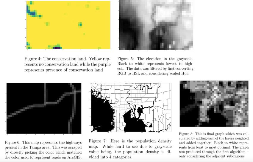
1. Proximity to a nearby motorway within the sub-regionTeam 14525 Page 13 2. Reserved conservation areas that prevent construction 3. Population density 4. Regional topography All of these metrics are found by using an ArcGIS program and layering the maps onto one another. We consider 1 and 2 to be Boolean such that the sub-region can either have a 0 or a 1 dependent on if the given sub-region contains the metric, provided by the ArcGIS program. The population density is calculated by dividing the population of a sub-region by the total area of a sub-region and is measured in people/square mile. These factors are evaluated by visualizing each of these factors layered on our three cities: Tampa, FL; New York City, NY; Chicago, IL. We found that ArcGIS contained each of these layers for each of our cities. Once the 4 layers for each of 3 cities were collected, we used OpenCV and Matplotlib in order to apply filters and convert the map and the colors to rankings and categorical data per 0.5 x 0.5 mile cubic area, to make the model more efficient for our data and and make it scalable. In order to convert the images into rankings. Population densities were divided into 5 categories: 0-5. 0 indicating no population density, and 5 indicating the highest population density. The conservation land and the highway lands were simplified to 0 or 1 for each of the 0.5 x 0.5 blocks (0 indicating no presence while 1 indicating presence). Once this data was collected and scaled, 2 different algorithms were considered. Both models didn’t consider the sub-regions which contained conservation areas for tower placement, but differed in the way they approached elevation. The first model con- sidered only the adjacent sub-region while calculating the score for each tower placement. The second model, however, considered all the grids top, down, right, left and the diagonals (stopping when the elevation went higher) while gradually decreasing the weight in order to simulate weak coverage. The grayscale images rendered by this algorithm are then fed into our custom Radial Cover- age Convergence (RCC) algorithm. The input images are minimally preprocessed via nearest neighbor rescaling to ensure integer computations can be used and that each pixel represent approximately a 1 × 1 mile region. The pixel values in the final preprocessed images rep- resent a tower dependency score with 0, black, being the lowest dependence, and 1, white, being the greatest dependence. The RCC algorithm then computes the cumulative radial area of each pixel in the image, with the radius being any given tower’s operative range. The position of the largest rendered value, say (x, y), is then selected for the emplacement of a cellular tower. The regional tower dependency around (x, y) is then muted, and the algorithm continues this process until a certain percentage of the total tower dependency score of the image is surpassed, usually 99%. A 100% coverage can be achieved, however, the return on investment to cover the remaining 1% may be undesireable. 3.5 Executing the Model The first model (the one with two algorithms on how to deal with adjacent sub-regions) was run on 3 cities: Tampa, FL; Chicago, IL; New York City, NY. The score calculated by
Team 14525                                                                          Page 14

each layer of data (score of reaching other regions - dependent upon elevation –, population
density, proximity to roads, land marked for conservation - automatic -) multiplied by their
weight were added together to calculate the score for each region. The graphs below show for
each city the filtered maps which were used for generating the rankings for each sub-region.
The visualizations will be presented in this order: Tampa, New York City, and Chicago.
Team 14525                                                                         Page 15

The model was also evaluated with the second algorithm (the one considering all the areas
surrounding each sub-region with lower elevations and gradually declining weight). Here are
the graphs for each of the cities.

The images were then fed into the RCC algorithm, and the tower positioning can be observed:
Team 14525                                                                           Page 16

3.6    Results and Discussion
Since the weight of population was double the weight of roads, the results seem optimal.
All the conservation areas were set to 0, which leads to purple holes in the final output. The
optimal placement seems to be in the inner areas of the city, where one can reach higher
elevation, and one where there is high population density. The data also aligns well with the
roads. Overall, a general trend can be seen, showing that the optimal placement is not on the
shores but in inner areas. However, in real life one can see that there is a higher
concentration of coverage on the shores than in the inner area. This could be due to per
capita income since it’s more optimal to target the wealthy, who are more likely to live on
the shores. However, in terms of covering as many people as possible, we can conclude that
the optimal place is in the areas marked as yellow.

It may be seen that the RCC algorithm places some cellular towers outside of inland areas.
Team 14525                                                                         Page 17
This is due to the input images containing marginal tower dependency scores offshore, which
was intended to account for the lower topographical potential enabling the signal to be
transmitted further.

3.6.1   Sensitivity Analysis
The sensitivity analysis was performed by adjusting the weights for population density and
roads. The last figures in the subsection Executing the Model were performed with the
weight for population density at 2, and for roads and highways it was 1. This could be
beneficial when considering rural areas because the traffic is likely not going to be very
high, thus less presence of people and activity. On the other hand, urban areas are likely to
have very high broadband usage on the highways and the roads. As a result, the optimal
placement would be better determined with higher weight on the roads. The grids represent
the optimal placement of towers, purple representing least optimal to yellow as the most
optimal.

Finally, suburban-urban areas are likely to contain both high population density and high
traffic. For these areas, it would be optimal to weight both the roads and the population
density the same. The resulting optimal tower placements for such cases are represented.

3.6.2   Strengths and Weaknesses
Our model is strong because we consider an iterative process that is predicated on finding
the maximum. Our data also takes into considering the topology of the area. Additionally,
the model is highly effective due to the raster analysis, which reduces the computational
speed tremendously. As a result, we can get the optimal 0.5 by 0.5 grid not only for cities
but even for countries and continents. The model also takes into account the decrease in
the strength of signal as one moves farther away from source or from potential buildings and
higher elevation areas. We also considered the areas which could not contain the cellular
towers.

One weakness is not considering the already covered area. As a result, this would have to
be done by the user himself/herself. We also didn’t take into account the cost of placing a
tower in different regions. We also assumed the height of the towers to be the same. We
utilized the data given in the M3 Excel sheet, D9, for approximating the megabits.

Finally, the model only determines the relative values and not absolute value. In other words,
it determines the best sub-region when compared to the other sub-region in the same map.
It could be possible that none of the region are optimally placed (for example all the sub-
regions would result in net loss for the company placing the towers).
Team 14525                                                                        Page 18

References
[1] Defeating the Digital Divide Data, MathWorks Math Modeling Challenge 2021,
    https://m3challenge.siam.org/node/523.

[2] https://drpeering.net/white-papers/Internet-Transit-Pricing-Historical-And-
    Projected.php.

[3] http://www.unisonsite.com/pdf/resource-center/How%20Towers%20Work.pdf.

[4] https://www.ppc-online.com/blog/nielsens-law-and-what-it-means-for-fiber-networks.

[5] https://www.investopedia.com/terms/l/lawofsupply.asp.

[6] https://www.ispreview.co.uk/index.php/2017/05/average-cost-per-mbps-uk-fixed-
    broadband-speed-0-34-vs-0-85-globally.html

[7] https://www.fcc.gov/consumers/guides/broadband-speed-guide.

[8] https://www.statista.com/statistics/323441/average-hours-worked-per-week-by-full-
    time-us-workers/.
Team 14525 Page 19
Code Used
Part 1
Part 2
import math
import random
import numpy as np
import matplotlib.pyplot as plt
global household
def mbps_education():
return np.random.normal(15, 5)
def mbps_work():
return np.random.normal(15, 5)
def mbps_recreation(age_bracket, isCovid, incomebracket):
if isCovid == False:
age_percent_time_spent_gaming = [0, 13.20271289, 25.05629478, 6.179310345, 2.251102344, 0.582398619, 0.192143467]
age_percent_time_spent_video = [0, 38.29691032, 59.14022518, 15.36551724, 9.979113483, 7.765314927, 7.301451751]
age_percent_time_spent_trad_tv = [0, 100, 100, 37.54482759, 46.27523787, 60.61259707, 72.37403928]
else:
age_percent_time_spent_gaming = [0, 12.10995542, 25.66462168, 5.341827983, 2.163511546, 0.536193029, 0.191901746]
age_percent_time_spent_video = [0, 46.50817236, 53.37423313, 21.46532713, 14.91574787, 8.789735733, 5.737862215]
age_percent_time_spent_trad_tv = [0, 100, 100, 38.15241362, 44.62242563, 54.76828801, 63.99923239]
income_percent_time_spent_gaming = [0, 9.856151371, 9.222945111, 7.278698946, 7.019600182]
income_percent_time_spent_video = [0, 28.92288007, 29.87033813, 28.69099963, 28.32910074]
income_percent_time_spent_trad_tv = [0, 78.06405335, 77.26793732, 74.61990782, 72.74532786]
activity = random.randint(1, 100)
if activityTeam 14525 Page 20
recreation_time_spent = math.floor(recreation(age_bracket) / 30)
bed_time = math.floor(bedtime(age_bracket) / 30)
# adds mbps for every hour of recreation until bedtime
while start_time 0:
household[start_time] += mbps_recreation(age_bracket, isCovid, incomebracket)
start_time += 1
recreation_time_spent -= 1
def initialize_fulltimejob(age_bracket):
temp = []
#age bracket
temp.append(age_bracket)
# work start time
# mean start time is 8:00 am with stddev of 10min
start_time = math.floor((np.random.normal(480, 10) / 30))
temp.append(start_time)
work_time_temp = random.randint(0, 100)
if work_time_tempTeam 14525 Page 21
while start_time 0:
household[start_time] += mbps_recreation(age_bracket, isCovid, incomebracket)
start_time += 1
recreation_time_spent -= 1
def unemployed_not_looking_for_work(age_bracket, isCovid, incomebracket):
recreation_time_spent = math.floor(recreation(age_bracket) / 30)
bed_time = bedtime(age_bracket)
start_time = math.floor((np.random.normal(480, 60) / 30))
# adds mbps for every hour of recreation until bedtime
while start_time 0:
household[start_time] += mbps_recreation(age_bracket, isCovid, incomebracket)
start_time += 1
recreation_time_spent -= 1
def initialize_ptepte(age_bracket):
temp = []
#age bracket
temp.append(age_bracket)
#school start time
# mean start time is 8:03 am with stddev of 11min
start_time = math.floor((np.random.normal(483, 11) / 30))
temp.append(start_time)
# mean amount of time at school is 6.64 hrs with stddev of .245 hrs
time_at_school = math.floor(np.random.normal(398.4, 14.7) / 30)
#school end time
school_end_time = start_time + time_at_school
temp.append(school_end_time)
# mean amount of time at work is between 1 and 7 hours
time_at_work = random.randint(1, 7)
temp.append(time_at_work)
return temp
def part_time_education_part_time_employment(age_bracket, start_time, school_end_time, time_at_work, isCovid, incomebracket):
while start_timeTeam 14525 Page 22
recreation_time_spent = np.random.normal(192.24, 60)
if age_bracket == 2:
recreation_time_spent = np.random.normal(139.68, 60)
if age_bracket == 3:
recreation_time_spent = np.random.normal(583.02, 60)
if age_bracket == 4:
recreation_time_spent = np.random.normal(686.4, 60)
if age_bracket == 5:
recreation_time_spent = np.random.normal(745.8, 60)
if age_bracket == 6:
recreation_time_spent = np.random.normal(744.92, 60)
return recreation_time_spent
def bedtime(age_bracket):
# based on age bracket, returns number of mins after time 0 at which individual goes to bed
if age_bracket == 1:
# mean 8 pm with stddev 1/3 hour
thebedtime = np.random.normal(1200, 20)
if age_bracket == 2:
# mean 10 pm with stddev 1/3 hour
thebedtime = np.random.normal(1320, 20)
else:
# mean 11 pm with stddev 1/3 hour
thebedtime = np.random.normal(1380, 20)
return thebedtime
def maximum():
maximum_val = 0
for x in range(len(household)):
if household[x] > maximum_val:
maximum_val = household[x]
return maximum_val
bins = []
for x in range(201):
bins.append(x / 2.0)
household = [0] * 48
maxvals = []
for x in range(300):
incomebracket = income_bracket()
initulfw = initialize_ulfw(3)
initfulltimejob = initialize_fulltimejob(3)
initfulltimeeducation = initialize_fulltimeeducation(1)
for x in range(365):
household = [0] * 48
unemployed_looking_for_work(initulfw[0], initulfw[1], initulfw[2], True, incomebracket)
fulltimejob(initfulltimejob[0], initfulltimejob[1], initfulltimejob[2], True, incomebracket)
fulltimeeducation(initfulltimeeducation[0], initfulltimeeducation[1], initfulltimeeducation[2], True, incomebracket)
maxvals.append(maximum())
a = np.array(maxvals)
mean = np.mean(a)
print("Scenario 1 mean is " + str(mean))
stddev = np.std(a)
print("Scenario 1 stddev is " + str(stddev))
ninetypercent = mean + 1.28155157 * stddev
print("90 percent of households in Scenario 1 will be satisfied with " + str(ninetypercent) + " Mbps")
ninetyninepercent = mean + 2.32634788 * stddev
print("99 percent of households in Scenario 1 will be satisfied with " + str(ninetyninepercent) + " Mbps")
plt.hist(a, bins = bins)
plt.xlabel("Maximum Daily Bandwith Used by Household Over the Course of a Year (Mbps)")
plt.ylabel("Number of Households")
plt.title("Scenario 1 (in the Presence of COVID-19)")
plt.show()Team 14525 Page 23
for x in range(300):
incomebracket = income_bracket()
initulfw = initialize_ulfw(3)
initfulltimejob = initialize_fulltimejob(3)
initfulltimeeducation = initialize_fulltimeeducation(1)
for x in range(365):
household = [0] * 48
unemployed_looking_for_work(initulfw[0], initulfw[1], initulfw[2], False, incomebracket)
fulltimejob(initfulltimejob[0], initfulltimejob[1], initfulltimejob[2], False, incomebracket)
fulltimeeducation(initfulltimeeducation[0], initfulltimeeducation[1], initfulltimeeducation[2], False, incomebracket)
maxvals.append(maximum())
a = np.array(maxvals)
mean = np.mean(a)
print("\nScenario 1 mean is " + str(mean))
stddev = np.std(a)
print("Scenario 1 stddev is " + str(stddev))
ninetypercent = mean + 1.28155157 * stddev
print("90 percent of households in Scenario 1 will be satisfied with " + str(ninetypercent) + " Mbps")
ninetyninepercent = mean + 2.32634788 * stddev
print("99 percent of households in Scenario 1 will be satisfied with " + str(ninetyninepercent) + " Mbps")
plt.hist(a, bins = bins)
plt.xlabel("Maximum Daily Bandwith Used by Household Over the Course of a Year (Mbps)")
plt.ylabel("Number of Households")
plt.title("Scenario 1 (Without the Presence of COVID-19)")
plt.show()
household = [0] * 48
maxvals = []
for x in range(300):
incomebracket = income_bracket()
initfulltimeeducation1 = initialize_fulltimeeducation(2)
initfulltimeeducation2 = initialize_fulltimeeducation(2)
for x in range(365):
household = [0] * 48
unemployed_not_looking_for_work(6, True, incomebracket)
fulltimeeducation(initfulltimeeducation1[0], initfulltimeeducation1[1], initfulltimeeducation1[2], True, incomebracket)
fulltimeeducation(initfulltimeeducation2[0], initfulltimeeducation2[1], initfulltimeeducation2[2], True, incomebracket)
maxvals.append(maximum())
a = np.array(maxvals)
mean = np.mean(a)
print("\nScenario 2 mean is " + str(mean))
stddev = np.std(a)
print("Scenario 2 stddev is " + str(stddev))
ninetypercent = mean + 1.28155157 * stddev
print("90 percent of households in Scenario 2 will be satisfied with " + str(ninetypercent) + " Mbps")
ninetyninepercent = mean + 2.32634788 * stddev
print("99 percent of households in Scenario 2 will be satisfied with " + str(ninetyninepercent) + " Mbps")
plt.hist(a, bins = bins)
plt.xlabel("Maximum Daily Bandwith Used by Household Over the Course of a Year (Mbps)")
plt.ylabel("Number of Households")
plt.title("Scenario 2 (in the Presence of COVID-19)")
plt.show()
for x in range(300):
incomebracket = income_bracket()
initfulltimeeducation1 = initialize_fulltimeeducation(2)
initfulltimeeducation2 = initialize_fulltimeeducation(2)
for x in range(365):
household = [0] * 48
unemployed_not_looking_for_work(6, False, incomebracket)
fulltimeeducation(initfulltimeeducation1[0], initfulltimeeducation1[1], initfulltimeeducation1[2], False, incomebracket)
fulltimeeducation(initfulltimeeducation2[0], initfulltimeeducation2[1], initfulltimeeducation2[2], False, incomebracket)Team 14525 Page 24
maxvals.append(maximum())
a = np.array(maxvals)
mean = np.mean(a)
print("\nScenario 2 mean is " + str(mean))
stddev = np.std(a)
print("Scenario 2 stddev is " + str(stddev))
ninetypercent = mean + 1.28155157 * stddev
print("90 percent of households in Scenario 2 will be satisfied with " + str(ninetypercent) + " Mbps")
ninetyninepercent = mean + 2.32634788 * stddev
print("99 percent of households in Scenario 2 will be satisfied with " + str(ninetyninepercent) + " Mbps")
plt.hist(a, bins = bins)
plt.xlabel("Maximum Daily Bandwith Used by Household Over the Course of a Year (Mbps)")
plt.ylabel("Number of Households")
plt.title("Scenario 2 (Without the Presence of COVID-19)")
plt.show()
household = [0] * 48
maxvals = []
bins = []
for x in range(51):
bins.append(x * 2)
for x in range(300):
incomebracket = income_bracket()
initialize_ptepte_1 = initialize_ptepte(3)
initialize_ptepte_2 = initialize_ptepte(3)
initialize_ptepte_3 = initialize_ptepte(3)
for x in range(365):
household = [0] * 48
part_time_education_part_time_employment(initialize_ptepte_1[0], initialize_ptepte_1[1], initialize_ptepte_1[2],
initialize_ptepte_1[3], True, incomebracket)
part_time_education_part_time_employment(initialize_ptepte_2[0], initialize_ptepte_2[1], initialize_ptepte_2[2],
initialize_ptepte_2[3], True, incomebracket)
part_time_education_part_time_employment(initialize_ptepte_3[0], initialize_ptepte_3[1], initialize_ptepte_3[2],
initialize_ptepte_3[3], True, incomebracket)
maxvals.append(maximum())
a = np.array(maxvals)
mean = np.mean(a)
print("\nScenario 3 mean is " + str(mean))
stddev = np.std(a)
print("Scenario 3 stddev is " + str(stddev))
ninetypercent = mean + 1.28155157 * stddev
print("90 percent of households in Scenario 3 will be satisfied with " + str(ninetypercent) + " Mbps")
ninetyninepercent = mean + 2.32634788 * stddev
print("99 percent of households in Scenario 3 will be satisfied with " + str(ninetyninepercent) + " Mbps")
plt.hist(a, bins = bins)
plt.xlabel("Maximum Daily Bandwith Used by Household Over the Course of a Year (Mbps)")
plt.ylabel("Number of Households")
plt.title("Scenario 3 (in the Presence of COVID-19)")
plt.show()
household = [0] * 48
maxvals = []
bins = []
for x in range(51):
bins.append(x * 2)
for x in range(300):
incomebracket = income_bracket()
initialize_ptepte_1 = initialize_ptepte(3)
initialize_ptepte_2 = initialize_ptepte(3)Team 14525 Page 25
initialize_ptepte_3 = initialize_ptepte(3)
for x in range(365):
household = [0] * 48
part_time_education_part_time_employment(initialize_ptepte_1[0], initialize_ptepte_1[1], initialize_ptepte_1[2],
initialize_ptepte_1[3], False, incomebracket)
part_time_education_part_time_employment(initialize_ptepte_2[0], initialize_ptepte_2[1], initialize_ptepte_2[2],
initialize_ptepte_2[3], False, incomebracket)
part_time_education_part_time_employment(initialize_ptepte_3[0], initialize_ptepte_3[1], initialize_ptepte_3[2],
initialize_ptepte_3[3], False, incomebracket)
maxvals.append(maximum())
a = np.array(maxvals)
mean = np.mean(a)
print("\nScenario 3 mean is " + str(mean))
stddev = np.std(a)
print("Scenario 3 stddev is " + str(stddev))
ninetypercent = mean + 1.28155157 * stddev
print("90 percent of households in Scenario 3 will be satisfied with " + str(ninetypercent) + " Mbps")
ninetyninepercent = mean + 2.32634788 * stddev
print("99 percent of households in Scenario 3 will be satisfied with " + str(ninetyninepercent) + " Mbps")
plt.hist(a, bins = bins)
plt.xlabel("Maximum Bandwith Used by Household at One Time (Mbps)")
plt.ylabel("Number of Households")
plt.title("Scenario 3 (Without the Presence of COVID-19)")
plt.show()
\end{lstlisting}
\subsection*{Part 3}
\begin{lstlisting}[language=Python]
# Beginning of ALGORITHM 1 --------------------- FOR PART 3
from cv2 import cv2
import numpy as np
import matplotlib.pyplot as plt
from PIL import Image
def evaluate_population_density (density_dir, width, height, graph=False):
img_den = Image.open(density_dir).convert('L').convert('RGB')
img = np.array(img_den)
for y in range(img.shape[1]):
for x in range(img.shape[0]):
if tuple(img[x][y]) == (246, 246, 246):
img[x][y] = 1
elif tuple(img[x][y]) == (206, 206, 206):
img[x][y] = 2
elif tuple(img[x][y]) == (165, 165, 165):
img[x][y] = 3
elif tuple(img[x][y]) == (113, 113, 113):
img[x][y] = 4
else:
img[x][y] = 0
img_den_sm = Image.fromarray(img).convert('L').resize((40, 27),resample=Image.BILINEAR)
np_img_den = np.array(img_den_sm)
if graph:
plt.figure(figsize=(20, 20))
plt.imshow(img * 63.75, cmap='gray')
return np_img_den
def evaluate_conservation_area (cons_dir, width, height, graph=False):Team 14525 Page 26
img = Image.open(cons_dir).convert('L')
img_sm = img.resize((47, 27),resample=Image.BILINEAR)
if graph:
plt.figure(figsize=(20, 20))
plt.imshow(img_sm)
im = np.array(img_sm)
ans = np.zeros((im.shape[0], im.shape[1]))
for y in range(im.shape[1]):
for x in range(im.shape[0]):
ans[x][y] = im[x][y] != 255
return ans
def evaluate_highway_area (high_dir, width, height, graph=False):
img = Image.open(high_dir).convert('RGB') #.convert('L')
img = np.array(img)
for y in range(img.shape[1]):
for x in range(img.shape[0]): # rgba(231,156,119,255)
if tuple(img[x][y][:3]) == (145,41,0):
img[x][y] = np.array([255, 255, 255])
elif np.sum(np.abs(img[x][y][:3] - np.array([231, 156, 119]))) < 10:
img[x][y] = np.array([255, 255, 255])
else:
img[x][y] = np.array([0, 0, 0])
img_sm = np.array(Image.fromarray(img).resize((40, 27), resample=Image.BILINEAR))
if graph:
plt.figure(figsize=(20, 20))
plt.imshow(img_sm)
ans = np.zeros((img_sm.shape[0], img_sm.shape[1]))
for x in range(img_sm.shape[0]):
for y in range(img_sm.shape[1]):
if tuple(img_sm[x][y]) != (0, 0, 0):
ans[x][y] = 1
else:
ans[x][y] = 0
return ans
def evaluate_elevation_area (elevation_dir, widht, height, graph=False):
img = Image.open(elevation_dir).convert('RGB')
img = cv2.cvtColor(np.array(img), cv2.COLOR_BGR2HLS)[:, :, 0]
img_sm = np.array(Image.fromarray(img).resize((40, 27), resample=Image.BILINEAR))
im = np.array(img_sm)
ans = np.zeros((im.shape[0], im.shape[1]))
if graph:
plt.figure(figsize=(20, 20))
plt.imshow(img_sm, cmap='gray')
img_sm = (img_sm - 13) / 101
return img_sm
def score_maps (a, b, c, d, width, height, grid_length, pw, hw, ew):
raw_score = np.zeros(a.shape)
for x in range(height):
for y in range(width):
if b[x][y] == 1:
continue
raw_score[x][y] += pw * a[x][y]
raw_score[x][y] += hw * c[x][y]Team 14525 Page 27
final_score = np.copy(raw_score)
for x in range(height):
for y in range(width):
if x != 0 and d[x][y] > d[x-1][y]:
final_score[x][y] += ew * raw_score[x-1][y]
if x != height-1 and d[x][y] > d[x+1][y]:
final_score[x][y] += ew * raw_score[x+1][y]
if y != 0 and d[x][y] > d[x][y-1]:
final_score[x][y] += ew * raw_score[x][y-1]
if y != width-1 and d[x][y] > d[x][y+1]:
final_score[x][y] += 0
plt.figure(figsize=(20, 20))
plt.imshow(final_score, cmap='gray')
plt.title("Optimal Placement of Cellular Towers")
plt.xticks([])
plt.yticks([])
density_dir = 'data/tampa/density-tampa.png'
cons_dir = 'data/tampa/cons-tampa.png'
high_dir = 'data/tampa/highway-tampa.png'
elevation_dir = 'data/tampa/elevation-tampa.png'
a = evaluate_population_density(density_dir, 40, 27, graph=True) # 1-4
b = evaluate_conservation_area(cons_dir, 40, 27, graph=True) # 0-1
c = evaluate_highway_area(high_dir, 40, 27, graph=True) # 0-1
d = evaluate_elevation_area(elevation_dir, 40, 27, graph=True) # 0-1
ans = score_maps(a, b, c, d, 40, 27, 1, 2, 1, 0.5)
density_dir = 'data/newyork/density-new-york.png'
cons_dir = 'data/newyork/cons-new-york.png'
high_dir = 'data/newyork/highway-new-york.png'
elevation_dir = 'data/newyork/elevation-new-york.png'
a = evaluate_population_density(density_dir, 40, 27, graph=True) # 1-4
b = evaluate_conservation_area(cons_dir, 40, 27, graph=True) # 0-1
c = evaluate_highway_area(high_dir, 40, 27, graph=True) # 0-1
d = evaluate_elevation_area(elevation_dir, 40, 27, graph=True) # 0-1
ans = score_maps(a, b, c, d, 40, 27, 1, 2, 1, 0.5)
density_dir = 'data/chicago/density-chicago.png'
cons_dir = 'data/chicago/cons-chicago.png'
high_dir = 'data/chicago/highway-chicago.png'
elevation_dir = 'data/chicago/elevation-chicago.png'
a = evaluate_population_density(density_dir, 40, 27, graph=True) # 1-4
b = evaluate_conservation_area(cons_dir, 40, 27, graph=True) # 0-1
c = evaluate_highway_area(high_dir, 40, 27, graph=True) # 0-1
d = evaluate_elevation_area(elevation_dir, 40, 27, graph=True) # 0-1
ans = score_maps(a, b, c, d, 40, 27, 1, 2, 1, 0.5)
def score_maps2 (a, b, c, d, width, height, grid_length, pw, hw):
raw_score = np.zeros(a.shape)
for x in range(height):
for y in range(width):
if b[x][y] == 1:
continue
raw_score[x][y] += pw * a[x][y]
raw_score[x][y] += hw * c[x][y]
final_score = np.copy(raw_score)
for x in range(height):
for y in range(width):Team 14525 Page 28
if b[x][y] == 1:
continue
cx = x + 1
c_ans = 0
while cx < height and d[cx][y] >= d[cx][y]:
curr_dist = np.abs(cx - x) / 2
if curr_distTeam 14525 Page 29
curr_dist = np.sqrt((cy-y)**2 + (cx-x)**2)
if curr_dist = d[cx][cy]:
curr_dist = np.sqrt((cy-y)**2 + (cx-x)**2)
if curr_dist = d[cx][cy]:
curr_dist = np.sqrt((cy-y)**2 + (cx-x)**2)
if curr_distTeam 14525 Page 30 c = evaluate_highway_area(high_dir, 40, 27) # 0-1 d = evaluate_elevation_area(elevation_dir, 40, 27) # 0-1 ans = score_maps2(a, b, c, d, 40, 27, 1, 2, 1) density_dir = 'data/tampa/density-tampa.png' cons_dir = 'data/tampa/cons-tampa.png' high_dir = 'data/tampa/highway-tampa.png' elevation_dir = 'data/tampa/elevation-tampa.png' a = evaluate_population_density(density_dir, 40, 27) # 1-4 b = evaluate_conservation_area(cons_dir, 40, 27) # 0-1 c = evaluate_highway_area(high_dir, 40, 27) # 0-1 d = evaluate_elevation_area(elevation_dir, 40, 27) # 0-1 ans = score_maps2(a, b, c, d, 40, 27, 1, 1, 2) density_dir = 'data/newyork/density-new-york.png' cons_dir = 'data/newyork/cons-new-york.png' high_dir = 'data/newyork/highway-new-york.png' elevation_dir = 'data/newyork/elevation-new-york.png' a = evaluate_population_density(density_dir, 40, 27) # 1-4 b = evaluate_conservation_area(cons_dir, 40, 27) # 0-1 c = evaluate_highway_area(high_dir, 40, 27) # 0-1 d = evaluate_elevation_area(elevation_dir, 40, 27) # 0-1 ans = score_maps2(a, b, c, d, 40, 27, 1, 1, 2) density_dir = 'data/chicago/density-chicago.png' cons_dir = 'data/chicago/cons-chicago.png' high_dir = 'data/chicago/highway-chicago.png' elevation_dir = 'data/chicago/elevation-chicago.png' a = evaluate_population_density(density_dir, 40, 27) # 1-4 b = evaluate_conservation_area(cons_dir, 40, 27) # 0-1 c = evaluate_highway_area(high_dir, 40, 27) # 0-1 d = evaluate_elevation_area(elevation_dir, 40, 27) # 0-1 ans = score_maps2(a, b, c, d, 40, 27, 1, 1, 2) density_dir = 'data/tampa/density-tampa.png' cons_dir = 'data/tampa/cons-tampa.png' high_dir = 'data/tampa/highway-tampa.png' elevation_dir = 'data/tampa/elevation-tampa.png' a = evaluate_population_density(density_dir, 40, 27) # 1-4 b = evaluate_conservation_area(cons_dir, 40, 27) # 0-1 c = evaluate_highway_area(high_dir, 40, 27) # 0-1 d = evaluate_elevation_area(elevation_dir, 40, 27) # 0-1 ans = score_maps2(a, b, c, d, 40, 27, 1, 2, 2) density_dir = 'data/newyork/density-new-york.png' cons_dir = 'data/newyork/cons-new-york.png' high_dir = 'data/newyork/highway-new-york.png' elevation_dir = 'data/newyork/elevation-new-york.png' a = evaluate_population_density(density_dir, 40, 27) # 1-4 b = evaluate_conservation_area(cons_dir, 40, 27) # 0-1 c = evaluate_highway_area(high_dir, 40, 27) # 0-1 d = evaluate_elevation_area(elevation_dir, 40, 27) # 0-1 ans = score_maps2(a, b, c, d, 40, 27, 1, 2, 2) density_dir = 'data/chicago/density-chicago.png' cons_dir = 'data/chicago/cons-chicago.png' high_dir = 'data/chicago/highway-chicago.png' elevation_dir = 'data/chicago/elevation-chicago.png' a = evaluate_population_density(density_dir, 40, 27) # 1-4 b = evaluate_conservation_area(cons_dir, 40, 27) # 0-1 c = evaluate_highway_area(high_dir, 40, 27) # 0-1 d = evaluate_elevation_area(elevation_dir, 40, 27) # 0-1 ans = score_maps2(a, b, c, d, 40, 27, 1, 2, 2)
Team 14525                                                                            Page 31
\end{lstlisting}

\begin{lstlisting}[language=Python]
import imageio as img
import tifffile as tif
import numpy as np

# ------- radial coverage convergence ----------------------------------
def radial_density_action(map_, pos, radius, action):
           height, width = map_.shape
           y, x = pos

          rad2 = radius * radius

          y1 = max(int(y - radius), 0)
          y2 = min(int(y + radius + 1), height)

          x1 = max(int(x - radius), 0)
          x2 = min(int(x + radius + 1), width)

          for oy in range(y1, y2):
                    dy = y - oy
                    dy2 = dy * dy

                     for ox in range(x1, x2):
                               dx = x - ox
                               dist2 = dy2 + dx * dx
                               if dist2 < rad2:
                                          action(map_, (oy, ox), map_[oy][ox])

def radial_density_sum(density_map, pos, radius):
         sigma = 0
         def _action(m, p, v):
                   nonlocal sigma
                   sigma += v

          radial_density_action(density_map, pos, radius, _action)
          return sigma

def radial_density_clear(density_map, pos, radius):
         sigma = 0
         def _action(m, p, v):
                   nonlocal sigma
                   y, x = p
                   sigma += m[y][x]
                   m[y][x] = 0

          radial_density_action(density_map, pos, radius, _action)

def get_radial_peaks(density_map, radius):
         height, width = density_map.shape
         peaks = []

          for y in range(height):
                    for x in range(width):
                              sigma = radial_density_sum(density_map, (y, x), radius)
                              peaks.append((sigma, (y, x)))

          # sort descending
          return list(sorted(peaks, key=lambda x: x[0], reverse=True))

def get_radial_peak(density_map, radius):
         height, width = density_map.shape
         max_sigma = None
         peak = None
You can also read