Assessing the accuracy of cosmological parameters estimated from velocity - density comparisons via simulations

MNRAS 000, 1–10 (2020) Preprint 13 January 2021 Compiled using MNRAS LATEX style file v3.0

 Assessing the accuracy of cosmological parameters estimated from
 velocity – density comparisons via simulations

 Amber M. Hollinger1,2 and Michael J. Hudson1,2,3
 1 Department of Physics and Astronomy, University of Waterloo, 200 University Ave W, Waterloo, ON N2L 3G1, Canada
 2 Waterloo Centre for Astrophysics, University of Waterloo, 200 University Ave W, Waterloo, ON N2L 3G1, Canada
 3 Perimeter Institute for Theoretical Physics, 31 Caroline St. North, Waterloo, ON N2L 2Y5, Canada
arXiv:2101.04120v1 [astro-ph.CO] 11 Jan 2021

 Accepted XXX. Received YYY; in original form ZZZ

 ABSTRACT

 A promising method for measuring the cosmological parameter combination 8 is to
 compare observed peculiar velocities with peculiar velocities predicted from a galaxy density
 field using perturbation theory. We use -body simulations and semi-analytic galaxy formation
 models to quantify the accuracy and precision of this method. Specifically, we examine a
 number of technical aspects, including the optimal smoothing length applied to the density
 field, the use of dark matter halos or galaxies as tracers of the density field, the effect of noise
 in the halo mass estimates or in the stellar-to-halo mass relation, and the effect of finite survey
 volumes. We find that for a Gaussian smoothing of 4ℎ−1 Mpc, the method has only small
 systematic biases at the level of 5%. Cosmic variance affects current measurements at the 5%
 level due to the volume of current redshift data sets.
 Key words: Galaxy: kinematics and dynamics – galaxies: statistics – large-scale structure of
 Universe – cosmology: observations

 1 INTRODUCTION Fundamental Plane standard candles/rulers) on their predicted pe-
 culiar velocities from the density field of galaxies, obtained from a
 Peculiar velocities are the only practical way of measuring the un-
 redshift survey. Specifically, the slope of this regression, , is then
 derlying distribution of dark matter (DM) on large scales (Willick
 combined with a measurement of the fluctuations of galaxies, 8, 
 et al. 1997), in the nearby (low redshift) Universe. Specifically, they
 to yield an estimate of
 can be used to measure the cosmological parameter combination
 (Ω ) 8 , where the first term is the logarithmic growth rate of 8 = 8, , (1)
 fluctuations, with (Ω ) = Ω0.55
 in the Lambda Cold Dark Mat-
 ter (ΛCDM) model, and 8 is the root mean square matter density as first suggested by Pike & Hudson (2005). The background theory
 fluctuation in a sphere of radius 8 ℎ−1 Mpc. Although peculiar ve- and assumptions implicit in this method are discussed in more detail
 locities have been used for similar purposes since the early 90s (see in Section 2 below.
 reviews by Dekel (1994) and Strauss & Willick (1995)), there has The goal of this paper is to test the accuracy and precision
 been a recent revival of interest in measuring 8 (Pike & Hudson of this method using large cosmological -Body simulations at a
 2005; Davis et al. 2011; Turnbull et al. 2012; Hudson & Turnbull redshift of zero of DM halos as a proxy for galaxies, as well as
 2012; Carrick et al. 2015; Huterer et al. 2017; Dupuy et al. 2019; semi-analytical models of galaxy formation. Our approach is not
 Qin et al. 2019; Adams & Blake 2020; Said et al. 2020; Boruah to simulate all the observational properties of the surveys simul-
 et al. 2020). taneously (as in, for example, Nusser et al. (2014)), but rather to
 The use of peculiar velocities as a probe of 8 has taken consider one by one the different physical effects which may bias
 on renewed importance in light of the 3.2 conflict between Cos- or add uncertainty to our results. In this sense the paper is similar
 mic Microwave Background (Planck Collaboration 2018) and weak in spirit to Berlind et al. (2000).
 lensing measurements (Asgari et al. 2019) of the parameter com- This paper is organized as follows. Section 2 describes the the-
 bination 8 ≡ Ω0.5 8 , with the latter giving lower values. This oretical framework of the relationship between peculiar velocities
 combination is very similar to 8 , differing by only 0.05 in the and the density fluctuation field from linear perturbation theory, and
 exponent of Ω . As shown by Boruah et al. (2020), some recent the relevant cosmological parameters. Section 3 presents the simu-
 peculiar velocity measurements also yield lower values of 8 than lation data and semi-analytic models that are used for the analyses
 Planck (as do most other probes of this parameter combination). performed in this paper. Section 4 describes the prescription for how
 One method for measuring 8 involves regressing the ob- we predict peculiar velocities. In section 5 we investigate how the
 served peculiar velocities (from e.g. supernovae, Tully-Fisher or choice of smoothing kernel impacts our estimates of / and the

 © 2020 The Authors

2 Hollinger and Hudson
amount of scatter generated in velocity – density cross-correlations. If linear biasing holds, then 8, = 8 . Putting this into equa-
Section 6 investigates how uncertainties corresponding to 0.1 and tion 7, we find that the product of the observables to be 8, ,
0.2 dex in halo mass measurements influence the predictions of / as in equation 1, and so we can set constraints on cosmological
and 8,h . In section 7 we instead explore how using either the stellar parameters.
to halo mass relation or galaxy observables to weight the density In reality, the assumptions of linearity, both in the context of
field impacts these cosmological estimates. Section 8 focuses on perturbation theory and in the context of biasing, will not hold
how these estimates are affected by volume limited surveys. Finally, exactly. Fortunately, peculiar velocities are primarily generated by
Section 9 presents our conclusions. large scale waves, where linearity will be a good approximation.
 Nevertheless, they also have a contribution from smaller, less linear
 scales. For these reasons, simulations are needed to calibrate any
2 PECULIAR VELOCITIES FROM LINEAR biases arising from non-linearities.
 PERTURBATION THEORY
In linear perturbation theory, it is possible to relate the density field
 3 SIMULATION DATA
to the peculiar velocities of the galaxies at low redshift using
 (Ω )
 ∫
 ( 0 − ) 3 0 We use two publicly available simulations: Bolshoi and MultiDark
 ( ) = 0 ( 0 ) 0 , (2) Planck 2 (MDPL2) (Klypin et al. 2011, 2016), along with two sim-
 4 | − | 3
 ulated semi-analytic catalogues, SAG (Cora et al. 2018) and SAGE
where ( ) is the peculiar velocity field and ( ) is the matter (Croton et al. 2016) which populate the DM haloes of MDPL2. We
density fluctuation field given by use the snapshots at = 0. The halo and galaxy catalogues were
 ( ) − ¯ obtained from the COSMOSIM database 1 .
 ( ) = , (3) The high-resolution Bolshoi simulation (Klypin et al. 2011)
 ¯
 follows 20483 particles in a comoving, periodic cube of length 250
where ( ) is the matter density field and ¯ is its cosmic average. ℎ−1 Mpc from = 80 to today. It has a mass and force resolution of
This calculation is only valid in the linear regime, where . 1, 1.35 × 108 ℎ−1 and 1 ℎ−1 kpc respectively, and the DM haloes
allowing higher order terms to be ignored (Peebles 1993). For ex- range from the masses of MW satellites (1010 ) to the largest
ample, it does not predict the transverse components of a galaxy of clusters (1015 ). It was run as a collisionless DM simulation
within a galaxy group. In ΛCDM, the rms matter density in spheres with the Adaptive Refinement Tree Code (ART; Kravtsov et al.
increases with decreasing sphere radius, so we expect linear theory (1997)) and assumes a flat, WMAP5 cosmology with parameters
to break down on small scales. In practice then, to apply equation 4 Ω = 0.27, ΩΛ = 0.73, ℎ = 0.7, (linear) 8 = 0.82 and = 0.95.
one needs to smooth ( ). Haloes in Bolshoi were identified using Rockstar (Behroozi et al.
 In the linear regime, the density modes in Fourier space grow 2013a). The (non-linear) 8, , measured from the particles is 0.897.
independently of one another. As a result it is easier to write equation The MultiDark project consists of a suite of cosmologi-
2 in Fourier space as follows cal hydrodynamical simulations (Klypin et al. 2016), all assume
 a flat ΛCDM cosmology with cosmological parameters: Ω =
 = 0 , (4) 0.307115, ΩΛ = 0.692885, ℎ = 0.6777, linear 8 = 0.8228, and
 | |2
 = 0.96, which is consistent with Planck results (Planck Collab-
where is the Hubble constant ( = 100 ℎ km s−1 Mpc−1 ). The oration 2018). We focus on the MDPL2 simulation which has a
smoothing is also simpler in Fourier space, because a convolution periodic box of length 1000 h−1 Mpc evolved from a redshift of 120
is a multiplication in Fourier space. to 0 with a varying physical force resolution level from 13-5 ℎ−1
 The density fluctuation field used in the previous equations is kpc and various implemented physics. The simulation uses 38403
that of the underlying matter density field. Because it is dominated dark matter particles of mass 1.51 × 109 ℎ−1 , and has identified
by dark matter, this cannot not be measured empirically. Instead, an more that 108 haloes using Rockstar (Behroozi et al. 2013a), with
assumption must be made as to how the observed galaxies trace the merger trees that were generated using ConsistentTrees (Behroozi
underlying total matter. If one assumes linear biasing, the relation et al. 2013b). The (non-linear) 8, , measured from the particles is
is 0.95.
 = , (5) The SAG (Cora et al. 2018) and SAGE (Croton et al. 2016)
 semi-analytic models include the most relevant physical processes
where is the linear bias and is the density fluctuation field of in galaxy formation and evolution, such as radiative cooling, star
the galaxies. Under this assumption equation 2 can be written as formation, chemical enrichment, supernova feedback and winds,
 (Ω )
 ∫
 ( 0 − ) 3 0 disc instabilities, starbursts, and galaxy mergers. These model were
 ( ) = 0 ( 0 ) 0 . (6) calibrated to generate galaxy catalogues using the MDPL2 simula-
 4 | − | 3
 tion. A comprehensive review of the models can be found in Knebe
Note that if we express distances in units of ℎ−1 Mpc (or km/s), et al. (2017).
as are naturally obtained from redshift surveys, then one must set
 = 100 km s−1 Mpc−1 (or 1, respectively) in the above expression.
Thus when applying this equation to density fields derived from 4 TESTING METHODS WITH N-BODY SIMULATIONS
redshift surveys, the predictions are independent of the true value
of . The other two values outside the integral can be compacted Our goal is to test equation (6) using data from N-body simulations.
into the parameter combination Specifically, we will calculate the predicted peculiar velocities by
 
 ≡ . (7) 1
 www.cosmosim.org

 MNRAS 000, 1–10 (2020)

Testing Accuracy of Peculiar Velocity Comparisons 3
integrating over a smoothed density tracer field, denoted by the velocity tracer, we linearly interpolate from the velocity grid to the
subscript “t”, used in place of ( ) in the integral, tracer’s location.
 As discussed above, we then regress the tracer velocity against
 ( 0 − ) 3 0
 ∫
 
 pred ( ) = 0 ( 0 ) 0 , (8) its predicted velocity, with the intercept fixed to zero, and where the
 4 | − | 3 fitted slope gives an estimate for . The fits also yield the rms (1D)
and compare this to the “observed” (unsmoothed) velocity tracers, velocity scatter, , of the difference between the -body velocities
which are used in place of ( ) on the left hand side of equation and the linear theory predictions at the best fit .
(6). Note that equation (8) omits the term, which we fit to the
N-body data by performing a linear regression
 5 THE EFFECT OF SMOOTHING LENGTH ON THE
 = pred , (9)
 ESTIMATED COSMOLOGICAL PARAMETERS
where is the measured N-body velocity of a tracer of the velocity As discussed above, the density tracer field must be smoothed in
field which, in principle, need not be the tracer as used for the den- order to predict the peculiar velocities in linear perturbation theory.
sity field). This is a cross-correlation between two samples, and we In this section, we assess the impact of different Gaussian smoothing
will refer to it generically as a velocity – density cross-correlation, lengths on the recovered value of , and the 1D around the linear
although the actual comparison is made between observed and pre- theory predictions. We focus on smoothing scales between 1-6 ℎ−1
dicted peculiar velocities. Mpc.
 The procedure used to obtain the density tracer field is the Specifically, we aim to confirm at what smoothing length the
same regardless of whether the tracer data are particles, DM haloes slope of linear regression is unbiased, which previous work has
or galaxies, as each simulation provides Cartesian positions and suggested lies in the range 4 – 5 ℎ−1 Mpc (Carrick et al. 2015).
velocities for all tracers. The latter two also provide additional in- We first consider particles as tracers of the density field, and then
formation such as halo mass, stellar mass and luminosity measure- consider haloes.
ments in different filter bands. In this paper, we will construct the
density fluctuation field using all of the aforementioned tracers. In
the following section however, we will focus solely on using the 5.1 Particle-weighted Density Fluctuation Field
particles for the density field.
 Likewise, one also has a choice of which velocity tracers to use We now consider the case in which we predict the peculiar velocities
in the comparison. Using the particles as the velocity tracers is the of particles using the particle density fluctuation field. The values
most straightforward, so we will begin with this case in Section 5.1 of the best-fit slope divided by the value of in the simulation,
below. Generally, however observers usually combine the peculiar i.e. / , as a function of smoothing scale, are shown in Figure 1.
velocities from multiple galaxies in the same group or cluster to ob- This quantity should be unity if the method is unbiased. We find
tain the mean peculiar velocity of the group. The -body analogue that predictions are unbiased for a Gaussian smoothing kernel 
for the group-averaged peculiar velocity is the peculiar velocity of between 4 and 5 ℎ−1 Mpc. Of the two simulations, MDPL2 should be
the host (or central) halo. more accurate since its minimum wavenumber is 2 ×10−3 ℎ/Mpc,
 In order to calculate the density field, the density tracers are and whereas that of Bolshoi is a factor 4 larger due to its smaller box
placed on a 3D cubic grid at the nearest grid point and the contri- length. Thus Bolshoi fails to capture the long-wavelength modes that
bution of all tracers at the same grid point is summed. generate a significant fraction of the rms peculiar velocity. The 1D
 In the case where grid spacing is non-negligible, the gridding around the best fit slope, however, is minimized at a smoothing
acts like smoothing, and it adds in quadrature with the applied to length that is 1-1.5 ℎ−1 Mpc smaller. The of particle peculiar
yield a total effective smoothing (Boruah et al. 2020), velocities is high: between 225 and 275 km/s. This is because the
 particle’s peculiar velocity includes its motion within the halo as
 2 2 2
 total = grid + smooth , (10) well as the peculiar velocity of the halo itself. Only the latter is
 well-predicted by linear perturbation theory.
 Δ2 If we predict the peculiar velocities of host (or central) haloes
 2 = grid where Δ
where grid −1
 12 grid is the grid spacing in ℎ Mpc.
 (i.e. excluding subhaloes) using the particle density field, we find
 Using a fine grid allows us to preserve some of the detail and
 similar results, with unbiased results and minimum occurring
ignore the effects of grid size smoothing. All comparisons in this
 for Gaussian smoothing lengths that are ∼ 0.5ℎ−1 Mpc smaller than
paper are done assuming a grid spacing of 0.36 and 0.98 h−1 Mpc
 when using particles as velocity tracers. The as a function of
for Bolshoi and MDPL2 respectively, which produces a negligible
 smoothing length is quite flat; it is not much higher at the fidu-
effect on the effective smoothing scales that will be used in this
 cial 4 ℎ−1 Mpc. However the amplitude of for host haloes is
paper.
 significantly lower (∼ 150 km/s) than for particles (∼ 250 km/s),
 We choose to smooth the density fluctuation field using a Gaus-
 as expected given that the velocities of the particles include their
sian smoothing kernel, which, in configuration and Fourier space,
 motion with respect to the host halo.
are given by
 Finally, it is interesting to explore the question of whether
 !
 1 − 2 haloes of different masses have different velocities relative to the
 ( ) = √ exp 2
 (11) predictions of linear theory, one scenario of “velocity bias.” We
 2 2 
 find that imposing a minimum mass threshold on the haloes used
 − 2 
 2 to sample the velocity field of 1012 has little effect on the
 !
 ( ) = exp , (12) measured / for smoothing lengths greater that 1.5 ℎ−1 Mpc for
 2
 MDPL2 and 3 ℎ−1 Mpc for Bolshoi, as shown in Fig. 2. This is also
respectively. We then calculate the peculiar velocities on the 3D true for a minimum mass of 1013 . A small velocity bias appears
grid using equation (4). To predict the peculiar velocity of a given only when considering cluster mass haloes (> 1014 ) as peculiar

MNRAS 000, 1–10 (2020)

4 Hollinger and Hudson

 1.1 1.1
 Slope of Linear Regression ( /f)

 Slope of Linear Regression ( /f)
 1.0
 0.9 1.0
 0.8
 0.9
 0.7
 0.6 0.8 MDPL2
 simulation : tracer
 0.5 MDPL2 : particles all haloes
 Bolshoi : particles 0.7 Mh>1012h 1M
 0.4 MDPL2 : haloes Mh>1013h 1M
 Bolshoi : haloes Mh>1014h 1M
 0.3 0.6
 325 200
 300 190
 275
 180
 250
[km/s]

 [km/s]
 170
 225
 160
 v

 200
 v

 175 150
 150 140
 125 130
 1 2 3 4 5 6 1 2 3 4 5 6
 Smoothing Length h 1Mpc Smoothing Length h 1Mpc

Figure 1. Top Panel: Slope of linear regression for the predicted and N-Body Figure 2. As in Fig. 1 where again the predicted peculiar velocities are
particle and central halo velocities (excluding subhaloes) for MDPL2 and based on the particle density field, but here these are compared to the -
Bolshoi simulations. Because we correct for the parameter, a value of / body peculiar velocities of haloes (but excluding subhaloes). For clarity the
of unity indicates for the smoothing length for which the velocity–density solid line labeled ’all halos’ represents all simulation objects classified as
cross-correlation is unbiased. The predicted velocities were calculated as- centrals, while the dashed lines represent centrals with masses greater than
suming an underlying particle density field and linear theory for the Gaussian various minimum masses as indicated in the legend.
smoothing radius shown on the horizontal axis . Bottom Panel: The scatter
between the measured -body and predicted peculiar velocity associated
with each of the linear regression slopes. A circle has been placed at the the method unbiased. This parameter combination will be referred
smoothing length where the standard deviation was minimized. to as ∗ = 8,m
 8,h
 .
 To measure 8 we placing non-overlapping spheres of 8
velocity tracers. For clusters, there is also an increase in the 1D ℎ−1 Mpc covering the entire the density field, and measure the
with respect to the linear theory predictions. standard deviation in the values. Doing this, we find values of
 8h = 1.45 ± 0.04 and 1.57 ± 0.02 for the halo masses for Bol-
 shoi and MDPL2 respectively, much larger than 8,m , which is the
5.2 Halo mass-weighted density field measured (non-linear) 8 of the particle density field.
 The fitted values of h / , however, are lower than unity, as
We now consider a scenario that is closer to the observational one, expected. The results for ∗ are plotted in Figure 3, showing that
where the density field is provided by DM haloes, weighted by their the mass-weighted determination is nearly unbiased: at the fiducial
mass. Whereas the particle density field is unbiased, this field will = 4ℎ−1 Mpc, the MDPL2 field has ∗ = 1.05, whereas for
be biased. Therefore, we no longer expect h / = 1. As discussed Bolshoi ∗ = 1.02. This suggests that linear biasing correction
above, in the linear regime, this bias can be calculated by measuring works well, even for fields with h ∼ 1.7. The 1D (∼ 160
the rms density fluctuations of the halo-weighted density field in 8 km/s) is only marginally higher than when particles were used for
ℎ−1 Mpc spheres. The halo and particle 8 measurements are related the density field.
by
 8,h
 h = (13)
 8,m 5.3 Discussion: Cross-Correlation and Optimal Smoothing
which is the same in the term defined previously. We measure It is not obvious why a Gaussian smoothing, with ∼ 3 − 4 ℎ−1
 / from the slope of linear regression as before, but multiplying Mpc, should be the “correct” smoothing length. We can gain some
this by the correction factor h . This should return a value of unity if insight by considering the problem in Fourier space, specifically

 MNRAS 000, 1–10 (2020)

Testing Accuracy of Peculiar Velocity Comparisons 5

 1.2

 1.0 1.0
 8, h/ 8, M)

 0.8 0.8
 ( /f) * (

 0.6 Minimum Halo Mass
 MDPL2 0.6
 Bolshoi
 0.4 all haloes
 Mh>1012h 1M 0.4

 240 0.2
 Zheng et al. 2013: W(k)
 220 e (kRG)2/2, RG = 2.88
Scatter [km/s]

 0.0 e (kRG)2/2, RG = 4.0
 200 10 2 10 1 100
 180
 k/h Mpc 1

 160
 Figure 4. The normalized window function from Zheng et al. (2013), cal-
 140 culated from the J1200 simulation, based on the correlation of the velocity
 and density fields (see text for details) is shown, with Window functions
 for Gaussian smoothing kernels with scales of 2.85 and 4.0 ℎ −1 Mpc. Both
 1 2 3 4 5 6
 Smoothing Length h 1Mpc functions exhibit the expected characteristics of being unity as → 0 and
 zero as → ∞. f and the Gaussian kernel of = 2.88 ℎ −1 Mpc cross
 0.5 near = 0.39 and 0.41ℎ/Mpc, respectively.

Figure 3. Similar to Fig. 2, except here the mass-weighted halo density field
is used to predict peculiar velocities of haloes. The vertical axis in the top plotted for comparison are two Gaussian smoothing filters with
panel is now / ( 8,ℎ / 8, ). = 2.88 and 4.0ℎ−1 Mpc. The estimated / from the par-
 ticle weighted density field smoothed using either e as a -
 space smoothing function or with a Gaussian kernel of = 2.88
equation 4 which relates the velocity modes to the density modes ℎ−1 Mpc both produce values of 0.88. There is also no significant
in linear perturbation theory. This should be exact on large scales, difference in .
but we expect it to break down at high . The Gaussian smoothing with = 4.0ℎ−1 Mpc is a better
 For simplicity, first assume that all Fourier modes are Gaus- match to e at low .
sian and independent and that at a given the joint distribution of In reality, particularly at high , the assumption of bivariate
velocity and density mode amplitudes is given by a bivariate Gaus- Gaussianity will no longer be correct, so the above simple argument
sian. We expect the correlation coefficient, , to approach 1 on large will break down. In principle, with detailed knowledge of the cor-
scales and zero at high . Generally if one has a bivariate normal relations, it should be possible to design the optimal -space filter.
distribution of two variables and , and one regresses on the For our purposes in this paper, we retain the simplicity of Gaussian
 
slope of the relation is , or since the covariance = , smoothing, and adopt a Gaussian smoothing filter with = 4
the slope can also be written / 2 . Therefore, the predicted ve- ℎ−1 Mpc for consistency with previous work.
locity mode amplitude is given by the density mode amplitude times
the slope / 2 .
 The quantities and 2 can be measured in -body simu- 6 THE EFFECT OF UNCERTAINTY IN THE HALO
lations as a function of wavenumber . The latter is just the power MASSES
spectrum of matter density fluctuations, , but the covariance
is less well studied. Zheng et al. (2013) have measured the cross- In the previous sections, the masses of the haloes were assumed to be
spectrum of the closely related quantity = ∇ · with the density known exactly, with no uncertainty in the measurements. However
 , and its ratio with the density power spectrum. They define the in real survey data there is a some uncertainty in the true mass of
normalized window function any given halo, depending on the method used to estimate it, and
 this may be in the range 0.1 – 0.2 dex (see Section 7). In this section,
e = 1 ,
 (14) we explore how scattering the halo mass impacts the predictions of
 
 / and 8,ℎ . This is accomplished by varying the halo masses
which has the property that it asymptotes to 1 at low and goes by a lognormal Gaussian random variable with standard deviations
to zero at higher . This function is plotted in Figure 4. Also over- corresponding to 0.1 and 0.2 dex, and calculating 8 and for each

MNRAS 000, 1–10 (2020)

6 Hollinger and Hudson

 1.14 Minimum Halo Mass
 Bolshoi:all haloes
 1.12 MDPL2:all haloes
 Bolshoi:1012h 1M SAGE
 MDPL2:1012h 1M
8, h/ 8, M)

 1.10 SAG
 12

 log(M* [h 1M ])
 1.08 10
/f * (

 1.06 8

 1.04 6
 165
 1.0
 160
 1.5
 155 log(M*/M*) 2.0
 [km/s]

 2.5
 150
 3.0
 145
 v

 3.5
 4.0
 140
 4.5
 135 10 11 12 13 14 15
 0.000 0.025 0.050 0.075 0.100 0.125 0.150 0.175 0.200 log(Mh [h 1M ]])
 scatter [dex]

Figure 5. Effect of additional scatter to the mass of haloes as a function of Figure 6. Top Panel: The stellar-to-halo mass relation (SHMR) for the total
the logarithmic scatter (0, 0.1 and 0.2 dex). For 0 dex this is the measured stellar mass of a halo (including stellar mass in subhaloes) as a function
value of the simulation, for 0.1 and 0.2 dex a random value corresponding of total halo mass. The dark curves show the means of the SHMR and the
to a lognormal Gaussian with a of ∼ 0.23 and 0.5 respectively, has lighter bands indicate their measured standard deviation. Both SAG and
been applied to each halo in the catalogue. Top panel: The mean (dark SAGE semi-analytic models are shown. Bottom Panel: the stellar to halo
line) and ±1 range (shaded band) of these measurements are shown for mass ratio as a function of halo mass.
 / ( 8,ℎ / 8, ) at a smoothing radius of 4 ℎ −1 Mpc. Bottom panel :
scatter around the best fit of for the same smoothing.
 to realization in h , h and their product ∗ . For MDPL2, the net
 effect of √
 scatter in the independent halo masses is reduced by a
realization. A total of 500 realizations were performed on both the factor 1/ due to the larger volume containing a larger number
Bolshoi and MDPL2 halo catalogues. of haloes. This highlights the importance of the volume of the
 We find that, from realization to realization, both the measured sample, a topic we shall discuss in greater detail in Section 8.
 and 8 deviate from the no-scatter values, and these deviations The bottom panel shows how the 1D is impacted by intro-
are anti-correlated. This can be understood as follows. In Section ducing stochasticity in the halo masses. We find that the 0.1 dex case
5.3, we discussed how the slope ( ) could be expressed as the ratio generates a negligible change in the measured when compared
of the covariance between density and velocity, and the density to the original value. For halo mass uncertainties of 0.2 dex, 
power spectrum, / 2 . If noise is added to the density field, increases, but the effect is still small, corresponding to ∼ 8 km/s.
then the denominator increases, but the covariance is unaffected.
Consequently, the fitted drops. On the other hand, 8 increases
because of the additional noise. This anti-correlation leads to some
 7 GALAXIES AS TRACERS OF THE DENSITY FIELD
cancellation of the additional noise from realization to realization
in the product ∗ = h 8,h . Galaxies trace the underlying dark matter distribution on large
 The net result of increasing the halo mass scatter and its impact scales, but observable quantities, such as a galaxy’s luminosity
on ∗ are shown in the top panel of Figure 5, with a scatter of zero and stellar mass, do not necessarily have an exact relationship with
dex corresponding to the case where the halo masses are precisely the mass of the halo in which a galaxy lies. To explore how using
measured. We find that when introducing a lognormal scatter, these quantities as a proxy for mass density impact / and 8 , we
 the value of ∗ increases only slightly with increasing scatter use two galaxy semi-analytic galaxy formation models available for
for both Bolshoi and MDPL2. We note however that the standard the MDPL2 simulation SAG (Cora 2006) and SAGE (Croton et al.
deviation of ∗ is higher for Bolshoi due to the smaller volume 2016).
of the simulation, which leads to greater variation from realization Many DM haloes host more than one galaxy, which are typ-

 MNRAS 000, 1–10 (2020)

Testing Accuracy of Peculiar Velocity Comparisons 7
 use these to convert the stellar masses into halo masses. Then the
 1.2 same analysis described in a previous section is performed. This
 1.1 procedure will remove the nonlinearity of the SHMR relation, but
 cannot remove the scatter in it, since the mean SHMR is used for
 1.0
 8, g/ 8, M)

 each halo.
 0.9 From Figure 7, we find for the SAGE galaxies, ∗ is unbiased
 for a Gaussian smoothing of 4.1 ℎ−1 Mpc but generates the lowest
 0.8 at = 2.6 ℎ−1 Mpc. For SAG these are at smoothing lengths of
 /f * (

 3.6 and 3.5 ℎ−1 Mpc, respectively. Comparing these results to Fig. 3,
 0.7 we find that at = 4 ℎ−1 Mpc, SAG produces results that are quite
 SAGE
 0.6 SAG similar (within a few percent) to what was found using MDPL2’s
 all haloes halo masses directly. SAGE, however, generates values of ∗ that
 0.5 Mh>1012h 1M are 5% smaller at the same smoothing length than the haloes. We
 find that the generated SAG haloes produce similar estimates for
 240 the 1D scatter in velocity predictions, contrarily the SAGE haloes
 generate ∼ 20 km/s less scatter.
 220 Comparing these results to those in the next section we note
 that while the halo mass does tend to be unbiased at smaller the
 200 conversion of stellar to halo mass introduces 10-20 km/s of addi-
[km/s]

 tional scatter than using galaxy observables to predicted velocities.
 We attribute the results to the differences in the models’ stellar
 180 to halo mass ratios as a function of halo mass. SAG has a flatter
 v

 stellar to halo mass ratio than SAGE, and therefore it is close to
 160 the simple halo mass weighted case. SAGE has a steeper ratio at
 high halo masses, hence SAGE puts less weight on massive clusters
 140 leading to estimates of ∗ slightly less than unity.

 1 2 3 4 5 6
 Smoothing Length h 1Mpc

 7.2 Predictions Using Galaxy Observables
Figure 7. Similar to Fig. 3, except here a fitted SHMR is used to predict
the halo masses from stellar masses, and then constructing a mass-weighted A density field can also be constructed without approximating the
halo density field to predict the peculiar velocities of central galaxies. mass of individual haloes via the SHMR. In this section, we in-
 vestigate how weighting directly by the galaxy observables impacts
 the cosmological estimates. Such a procedure is closer to what was
ically divided into centrals (the galaxy identified with the main or done by Carrick et al. (2015), who used the -band luminosity-
host DM halo) and satellites (associated with DM subhaloes). When weighted density field from the 2M++ catalogue. Figure 8 shows
predicting host halo mass, one can use only the stellar mass or lu- the summary of results discussed below.
minosity of the central galaxy, or one can use the total stellar mass We find that, for the SAG model, weighting the density field by
(or total luminosity) of all galaxies. We adopt the latter approach stellar mass produces results that yield a higher ∗ than luminosity
here when calculating the density fields. As before, velocity com- weighting. We can weight the density field using luminosities in any
parisons will be done solely on galaxies classified as centrals. For of the five bands provided by SAG. In the remainder of this paper we
consistency with the previous work done in this paper, any cuts focus on the -band luminosity. We note however that the longest
imposed on the data will be done using the mass of the host halo. wavelength -band produces the highest values of / however
 The stellar to halo mass relation (SHMR) is different for both after applying the correction factor ( 8,g / 8,m ) there is virtually
the SAG and SAGE semi-analytic models in MDPL2, see 6. SAG no difference between bands for ∗ , provided a low minimum mass
has a tighter SHMR with less scatter in stellar mass at a given halo threshold.
mass: for haloes with masses between 1011 and 1013 ℎ−1 , it If the minimum mass threshold of the haloes is low, we find
has an average scatter of 0.15 dex compared to 0.39 dex in SAGE. that weighting using the stellar masses provided by SAG closely
The average SHMR is comparable for both SAG and SAGE for halo resembles the case where the density field is halo-mass weighted
masses greater than the characteristic pivot point at ∼ 1012 ℎ−1 . and is unbiased at an ∼ 3.8 ℎ−1 Mpc. The SAGE stellar mass
 and SAG -band predict ∗ values that are comparable at > 3
 ℎ−1 Mpc, but only produce unbiased estimated of ∗ for a Gaussian
7.1 Predictions using Stellar-to-Halo Mass Relations
 smoothing radius of ∼ 5 ℎ−1 Mpc.
To construct a proxy mass density field, we can obtain proxy halo In the case where a minimum mass threshold of 1012 ℎ−1 is
masses using the SHMR. The K-band luminosity is a good proxy applied to the data, we find that ∗ for the three cases are comparable
for stellar mass, however the galaxy luminosities in SAG are limited for 3ℎ−1 Mpc . . 4ℎ−1 Mpc. With all the cases estimating
to the , , , , -bands. So in this section, we use the stellar masses unbiased ∗ values at 3.5-3.7 ℎ−1 Mpc. The is also comparable
provided for both SAG and SAGE. We fit the SHMR profiles of both for these cases with the SAGE stellar mass producing only ∼ 10
SAG and SAGE semi-analytic models with a broken power law, and km/s less scatter than the SAG -band.

MNRAS 000, 1–10 (2020)

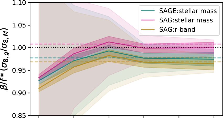
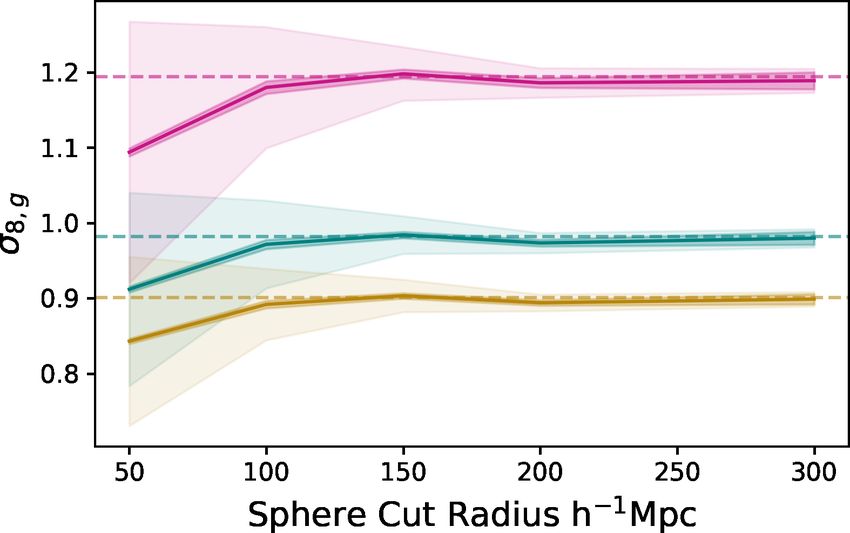
8 Hollinger and Hudson

Table 1. Summary of ∗ values taken for = 4 ℎ −1 Mpc for the various MDPL2 tracers which weight the density field and from which the peculiar velocities
are compared.

 Density Tracer all M > 1012 ℎ −1 

 Particles 0.97 – Figure 1
 Haloes 1.05 1.08 Figure 3
 SAGE: SHMR 1.00 1.02 Figure 7
 SAG: SHMR 1.04 1.06 Figure 7
 SAGE: stellar mass 0.98 1.01 Figure 8
 SAG: stellar mass 1.01 1.03 Figure 8
 SAG: -band luminosity 0.97 1.02 Figure 8

 1.1

 1.0
 8, g/ 8, M)

 0.9

 0.8
 /f * (

 SAG: rband
 0.7 SAG: stellar mass
 SAGE: stellar mass
 0.6 all haloes
 Mh>1012h 1M

 200

 180
[km/s]

 160
 v

 140

 120
 1 2 3 4 5 6
 Smoothing Length h 1Mpc

Figure 8. Similar to Fig. 7 except now the density field is constructed using Figure 9. To demonstrate the dependence of our calculated parameters on
galaxy observables (i.e. weighted by stellar mass or luminosity) to predict the survey volume, we restrict simulation data to (non-overlapping) spheres
and measure centrals’ peculiar velocities. of radius ranging from 50 to 300 ℎ −1 Mpc. The components of ∗ are
 calculated for each test sample assuming a Gaussian smoothing kernel of 4
 ℎ −1 Mpc. The upper panel and lower panel show the results for ∗ and in 8
 measurements, respectively, as a function of sphere radius. In both panels,
8 FINITE VOLUME AND COSMIC VARIANCE EFFECTS the light and dark coloured bands represent the ±1 standard deviation
 from sphere to sphere and the standard error in the mean of the test cases
In real data sets both the data used to obtain the density field, based
 (respectively) for a given sample spherical radius, with the mean being
on redshift surveys, and the peculiar velocity samples, cover limited
 shown by the solid colour lines. The colour horizontal dashed lines show
volumes. This has multiple consequences. Some of these are related the values from the full simulation box.
to sample variance: the local volume will have local values of the
mean density and of 8 that are different from the global values.
Moreover, the predicted peculiar velocities will be less accurate for 100, 150, 200 and 300 ℎ−1 Mpc, and its impact on cosmological
galaxies close to the edge of the density field than for those far from estimates. In particular, we are interested in simulations of data sets
the edges, say at the center of the volume. with max ∼ 150ℎ−1 Mpc, which is comparable to the survey size
 In this section, we investigate these finite volume and edge of 2M++, the depth of which varies from 125 ℎ−1 Mpc to 200 ℎ−1
effects by limiting the data, to spheres of radii with max = 50, Mpc, with an effective spherically-averaged radius of 175 ℎ−1 Mpc.

 MNRAS 000, 1–10 (2020)

Testing Accuracy of Peculiar Velocity Comparisons 9

 1.2 from sample variance effects, which is a combination of cosmic
 variance in the underlying DM structures and stochasticity in the
 1.1 SHMR. This decreases as max increases.
 Likewise, the locally-measured value of / also varies from
 1.0 sphere to sphere. Again, there are several reasons for this. First, the
 8, g/ 8, M)

 local ¯ averaged over the sphere will differ from the true average.
 0.9
 This is important because, as noted above, it leads to a renormal-
 0.8 ization of . Second, there is also stochasticity in the SHMR which
 /f * (

 may affect the locally-measured / . Of these two, the first ef-
 0.7 fect is the dominant one: we find that the total scatter in / for
 max = 150ℎ−1 Mpc at = 4ℎ−1 Mpc is typically 7.0% and is
 0.6 SAGE: stellar mass mostly due to cosmic variance in . ¯ The scatter in / dominates
 SAG: stellar mass
 0.5 SAG: r-band the scatter in 8,g (2.5%) when they are combined in ∗ .
 Figure 10 demonstrates how the cut samples ( max = 150ℎ−1
 Mpc) depend on the Gaussian smoothing radius . In particular,
 when compared to Figure 8 we find that the average ∗ for these
 240
 volume-limited realizations are unbiased between 3.75-4.75 ℎ−1
 Mpc. The value of ∗ at = 4ℎ−1 Mpc ranges between 0.98-1.01.
 220 More importantly, the standard deviation in ∗ from sphere to sphere
 is 0.077 at max = 150ℎ−1 Mpc, although this declines significantly
[km/s]

 to 0.032 at 200 ℎ−1 Mpc and 0.020 at 300 ℎ−1 Mpc. This suggests
 200
 that sample variance effects are the dominant uncertainty in 8
 v

 for current data sets.
 180 The 1D velocity scatter as a function of has a similar
 shape as found previously, but is 40-50 km/s larger than for the
 full simulation box. This increase in the scatter is primarily due
 160 to the degradation of the predicted velocities as one approaches
 max . When we compare the 1D for the subsample of galaxies
 1 2 3 4 5 6
 Smoothing Length h 1Mpc located within the inner half of the sphere’s volume with those in
 the outer half at an = 4ℎ−1 Mpc, we find scatters of ∼ 165 km/s
 and ∼ 210 km/s, respectively. This increase is attributed to the fact
 that the velocity tracers near the outer edge have poorer predicted
Figure 10. Similar to Fig. 8 expect we now use non-overlapping sphere cuts peculiar velocities because of unaccounted-for structures outside of
of radius 150 ℎ −1 Mpc and the components of ∗ are calculated for a range the survey limits.
of Gaussian kernel lengths between 1-6 ℎ −1 Mpc. The bands have the same
meaning as in Fig. 9.

Given the size of the MDPL2 simulation, it is possible to generate 9 SUMMARY AND DISCUSSION
multiple independent (non-overlapping) finite volume realizations. The key results of this paper are as follows:
For each sphere, we ignore any galaxy that exists outside of the
sphere, and assign = 0 for points outside the sphere. Hence each • The velocities of DM haloes are well predicted by linear theory
sphere represents a local universe realization: it can be over- or from the true density field with a Gaussian smoothing = 4ℎ−1
underdense, so we renormalize using the mean density within Mpc with a velocity scatter of 154 km/s. This is in agreement with
the sphere instead of the simulation box average. For each sphere, Appendix A of Carrick et al. (2015).
we then calculate / and 8,g using only that sphere’s galaxies, • This can be understood because, in Fourier space, a Gaussian
although 8, , which appears in the denominator of ∗ , continues filter with = 3 – 4 ℎ−1 Mpc is a good match to the cross-
to be calculated from the full simulation. As in real analyses, to correlation function of the density and velocity fields.
account for the missing contribution from structures beyond the • The accuracy and precision of the linear theory predictions do
sphere’s edge, in addition to fitting the / , we also fit a residual not depend on the mass of the velocity tracer; there is no "velocity
bulk flow term. bias", except for clusters with h > 1014 ℎ−1 .
 Figure 9 demonstrates how ∗ and 8,g depend on max for • If DM haloes are used as tracers of the density field, and one
the case with no mass cut on the galaxy catalogue. As expected, as calculates 8,h of the halo-mass-weighted density field, then h 8,h
the size of the sphere increases, results converge to the values found is a good estimator of 8 .
for the full simulation for max ≥ 200ℎ−1 Mpc. • If noise is added to the DM halo masses, then ∗ is biased high
 There is a significant amount of scatter in the measured 8 by only a percent, for a 0.1 dex noise level.
values for small max , varying by as much as 10% of the mean • When galaxy luminosity or stellar mass are used for the density
value, and with a mean value that tends to be between 4-8 % lower field, the values of ∗ indicate that the method is unbiased to within
than that of the full simulation. The bias in the mean may be due to 5%, depending on the semi-analytic galaxy formation model.
renormalizing the density fluctuation, = ( − )/
 ¯ ¯ with the local ¯ • When the density field is restricted to a finite volume, there is
measured on the scale of the sphere, max , thus effectively filtering additional uncertainty due to cosmic variance, at the level of 7% for
out the contribution to 8 from large-scale waves. The scatter arises a 150 ℎ−1 Mpc sphere.

MNRAS 000, 1–10 (2020)

10 Hollinger and Hudson
 The results for ∗ calculated using the same tracers for the Asgari M., et al., 2019, KiDS+VIKING-450 and DES-Y1 com-
velocity and density field, are summarised in Table 1. Overall we bined: Mitigating baryon feedback uncertainty with COSEBIs
find that the method has ∼ 5% systematic uncertainties. This can (arXiv:1910.05336)
be improved with semi-analytic galaxy formation models that more Behroozi P. S., Wechsler R. H., Wu H.-Y., 2013a, ApJ, 762, 109
carefully match the real SHMR and its scatter. There is also uncer- Behroozi P. S., Wechsler R. H., Wu H.-Y., Busha M. T., Klypin A. A.,
 Primack J. R., 2013b, ApJ, 763, 18
tainty due to finite volumes and cosmic variance.
 Berlind A. A., Narayanan V. K., Weinberg D. H., 2000, ApJ, 537, 537
 Previous work has neglected the additional scatter due to the Boruah S. S., Hudson M. J., Lavaux G., 2020, MNRAS, 498, 2703
coupled effects of stochasticity in the galaxy-mass relation and the Carrick J., Turnbull S. J., Lavaux G., Hudson M. J., 2015, Monthly Notices
cosmic variance effect of finite volumes. For example, the 2M++ of the Royal Astronomical Society, 450, 317
catalogue (Lavaux & Hudson 2011) has an effective volume of Cora S. A., 2006, MNRAS, 368, 1540
175 ℎ−1 Mpc. The SAGE model, weighted by stellar mass, shows Cora S. A., et al., 2018, Monthly Notices of the Royal Astronomical Society,
that, for 150 ℎ−1 Mpc spheres, the uncertainty on g 8, = 8 479, 2–24
is 7.7%, while the expected (interpolated) value for a survey of Croton D. J., et al., 2016, The Astrophysical Journal Supplement Series,
2M++’s size is 5.2%. This is slightly higher than the uncertainty 222, 22
 DESI Collaboration et al., 2016, arXiv e-prints, p. arXiv:1611.00036
estimated by Carrick et al. (2015), Boruah et al. (2020) and Said
 Davis M., Nusser A., Masters K. L., Springob C., Huchra J. P., Lemson G.,
et al. (2020) who adopted a 4% sampling variance uncertainty, plus
 2011, MNRAS, 413, 2906
observational errors in due to uncertainties in peculiar velocity Dekel A., 1994, ARA&A, 32, 371
measurements, which are subdominant. For precise quantification Dupuy A., Courtois H. M., Kubik B., 2019, MNRAS, 486, 440
of the biases and systematic uncertainties in 8 derived from a Hudson M. J., Turnbull S. J., 2012, The Astrophysical Journal Letters, 751,
specific survey, e.g. 2M++, the best approach to minimizing the L30
systematic errors will be to create mock catalogues that mimic the Huterer D., Shafer D. L., Scolnic D. M., Schmidt F., 2017, J. Cosmology
geometry and selection of that particular survey. Astropart. Phys., 2017, 015
 The cosmic variance uncertainty can be reduced in the future Klypin A. A., Trujillo-Gomez S., Primack J., 2011, ApJ, 740, 102
with deeper, all-sky redshift surveys. For example, a survey extend- Klypin A., Yepes G., Gottlöber S., Prada F., Heß S., 2016, MNRAS, 457,
 4340
ing to a redshift of 0.2 (600 ℎ−1 Mpc) would have an uncertainty of
 Knebe A., et al., 2017, Monthly Notices of the Royal Astronomical Society,
only 0.4% in the mean mass density and hence 0.5 – 0.6% in the
 474, 5206–5231
luminosity (or stellar mass) density. In the North, the DESI Bright Kravtsov A. V., Klypin A. A., Khokhlov A. M., 1997, The Astrophysical
Galaxy Survey (DESI Collaboration et al. 2016), will observe 10 Journal Supplement Series, 111, 73–94
million nearby galaxies. In the South, 4MOST (de Jong et al. 2019) Lavaux G., Hudson M. J., 2011, Mon. Not. R. Astron. Soc., 416, 2840
has the capability to survey large volumes in the nearby Universe. Nusser A., Davis M., Branchini E., 2014, ApJ, 788, 157
The future looks bright. Peebles P. J. E., 1993, Principles of physical cosmology. Princeton University
 Press
 Pike R., Hudson M. J., 2005, The Astrophysical Journal, 635, 11
 Planck Collaboration 2018, arXiv e-prints, p. arXiv:1807.06209
ACKNOWLEDGEMENTS Qin F., Howlett C., Staveley-Smith L., 2019, MNRAS, 487, 5235
 Said K., Colless M., Magoulas C., Lucey J. R., Hudson M. J., 2020, MNRAS,
MJH acknowledges support from an NSERC Discovery grant. 497, 1275
 The CosmoSim database used in this paper is a service by the Strauss M. A., Willick J. A., 1995, Phys. Rep., 261, 271
Leibniz-Institute for Astrophysics Potsdam (AIP). The MultiDark Turnbull S. J., Hudson M. J., Feldman H. A., Hicken M., Kirshner R. P.,
database was developed in cooperation with the Spanish MultiDark Watkins R., 2012, MNRAS, 420, 447
Consolider Project CSD2009-00064. The authors gratefully ac- Willick J. A., Courteau S., Faber S., Burstein D., Dekel A., Strauss M. A.,
knowledge the Gauss Centre for Supercomputing e.V. (www.gauss- 1997, The Astrophysical Journal Supplement Series, 109, 333
centre.eu) and the Partnership for Advanced Supercomputing in Zheng Y., Zhang P., Jing Y., Lin W., Pan J., 2013, Physical Review D, 88
Europe (PRACE, www.prace-ri.eu) for funding the MultiDark sim- de Jong R. S., et al., 2019, The Messenger, 175, 3
ulation project by providing computing time on the GCS Super-
computer SuperMUC at Leibniz Supercomputing Centre (LRZ, This paper has been typeset from a TEX/LATEX file prepared by the author.
www.lrz.de).
 The Bolshoi simulations have been performed within the Bol-
shoi project of the University of California High-Performance Astro
Computing Center (UC-HiPACC) and were run at the NASA Ames
Research Center.

DATA AVAILABILITY STATEMENT
The data underlying this article are publicly available from the
COSMOSIM database https://www.cosmosim.org/, with their
respective publications cited in section 3.

REFERENCES
Adams C., Blake C., 2020, MNRAS,

 MNRAS 000, 1–10 (2020)