Developing an Aerial-Image-Based Approach for Creating Digital Sidewalk Inventories - CE-CERT
←
→
Page content transcription
If your browser does not render page correctly, please read the page content below
Research Article

                                                                                                        Transportation Research Record
                                                                                                        2019, Vol. 2673(8) 499–507
                                                                                                        Ó National Academy of Sciences:
Developing an Aerial-Image-Based                                                                        Transportation Research Board 2019
                                                                                                        Article reuse guidelines:
Approach for Creating Digital Sidewalk                                                                  sagepub.com/journals-permissions
                                                                                                        DOI: 10.1177/0361198119842820

Inventories                                                                                             journals.sagepub.com/home/trr

Ji Luo1, Guoyuan Wu1, Zhensong Wei1, Kanok Boriboonsomsin1,
and Matthew Barth1

Abstract
To support active mobility, extensive work has been focused on planning, maintaining, and enhancing infrastructure, such as
sidewalks. A significant amount of these efforts has to go on the setup and maintenance of sidewalk inventory on a certain
geographic scale (e.g., citywide, statewide). To address the stated problem, this paper proposes the development of an aerial-
image-based approach that can 1) extract the features of sidewalks based on digital vehicle road network; 2) overlay the initial
sidewalk features with aerial imagery and extract aerial images around the sidewalk area; 3) apply a machine learning algo-
rithm to classify sidewalk images into two major categories, that is, concrete surface present or sidewalks missing; and 4)
construct a connected sidewalk network in a time-efficient and cost-effective manner. A deep convolutional neural network
is applied to classify the extracted sidewalk images. The learning algorithm gives 97.22% total predication rate for the test set
and 92.6% total predication rate in the blind test. The proposed method takes full advantage of available data sources and
builds on top of the existing roadway network to digitize sidewalks.

Ever-increasing transportation activities have raised a                   and even pose safety risks to those vulnerable road
range of public concerns such as increasing traffic con-                  users, since a portion of the path may not be walk-
gestion and degraded air quality. As one of the promising                 able or be in conflict with motor vehicles. In such
remedies, active mobility such as walking and bicycling                   cases, an accurate (connected) sidewalk network
are advocated to provide various environmental, public                    becomes necessary.
health, and economic benefits (1, 2). To promote the                     Crowdsourcing-based sidewalk inventory mainte-
active transportation mode, extensive work has been                       nance and update: as aforementioned, a large-
focused on planning and developing pedestrian- and                        scale sidewalk inventory will facilitate the mainte-
bicyclist-related programs which require infrastructure                   nance or improvement of existing sidewalks and
such as sidewalks and associated information as the cor-                  planning of new sidewalk construction. For exam-
nerstones. Significant efforts were made for the setup,                   ple, based on the updated digitized sidewalk net-
maintenance, and evaluation of the sidewalk inventory                     work database, active travelers and traffic
on a relatively large geographic scale (e.g., citywide, sta-              engineers can identify or report damaged side-
tewide). Based on a previous study (3), this paper applied                walks and share the locations in a timely and cost-
a more advanced method to create such a sidewalk inven-                   effective manner.
tory. The sidewalk information potentially lays a solid
foundation for a variety of active-mobility-focused appli-        Conventionally, traffic engineers and researchers have to
cations and related research, for example:                        rely on field measurements to conduct sidewalk survey
                                                                  and assessment (4, 5), which is rather resource
      Improved location-awareness service: as illustrated
       in Figure 1, the state-of-the-art navigation tools,
                                                                  1
       e.g., Google Maps (https://www.google.com/                  College of Engineering, Center for Environmental Research & Technology,
                                                                  University of California, Riverside, Riverside, CA
       maps), rely on the roadway network, which is
       designed for vehicles, to guide pedestrians.               Corresponding Author:
       Some navigation instructions can be confusing              Address correspondence to Ji Luo: ji.luo@ucr.edu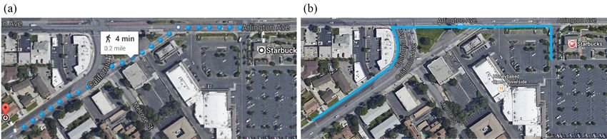
500                                                                                         Transportation Research Record 2673(8)

Figure 1. A comparative example on pedestrian navigation using (a) existing roadway network and (b) potential sidewalk network (from
National Center for Sustainable Transportation [3]).

consuming, regarding both time and cost. Recently, a                using the roadway (10). In an urban or suburban envi-
few studies attempted to collect the pedestrian volume              ronment, the sidewalk segments usually exist parallel to
and bicycle lane inventory with crowd-sourced informa-              the vehicle roadways and are largely associated with the
tion (6, 7), or synthesize digital sidewalk inventory based         roadway network. In addition, it is not straightforward
on commonly available open data (8). However, most of               to predict whether the sidewalk sections are present or
the existing methods for sidewalk system digitization are           not merely based on the surrounding roadway and land
neither comprehensive nor cost-effective at city-wide               use information. Therefore, it is of great interest to clas-
scales.                                                             sify the initialized sidewalk sections into paved (concrete
   On the other hand, thanks to the rapid advances in               surface present) and sidewalk missing (concrete surface
computational capability and explosion of data availabil-           does not exist) categories as a first attempt. In this
ity, machine learning techniques have shown great poten-            paper, unless otherwise noted, the phrases ‘‘paved’’ and
tial for image recognition and classification (9). To               ‘‘concrete-surfaced’’ are interchangeable, and ‘‘missing’’
address the above issues, we propose an aerial-image-               means that the sidewalk surfaces do not exist.
based sidewalk digitization method which is more time-                  The overall method is illustrated in Figure 2. In this
efficient and cost-effective than existing methods. The             study, we proposed to map the features of sidewalks
basic idea is to take full advantage of existing vehicle            based on the roadway network as the first step. The road-
roadway networks to reconstruct an initial (connected)              way network data applied in this study, such as roadway
sidewalk network. Then, the machine learning technique              shapefiles, should include road link attributes and posi-
is applied to the aerial images of focused areas (i.e., sur-        tion coordinates (11). Secondly, a Python script was writ-
rounding zones along the initial sidewalk network) to               ten to sweep each sidewalk link in the initialized sidewalk
identify whether a sidewalk is present or not.                      network and extract the aerial image within that area. In
   The paper is organized as follows: First is an over-             parallel, we manually classified a large number of aerial
view of the proposed methodology for sidewalk digitiza-             images (e.g., paved or missing sidewalk) of sidewalk net-
tion. Then the paper will illustrate how to construct a             work and set up a machine learning algorithm to learn
connected sidewalk network (as an initial) by mapping               from the labeled images. We trained the machine learning
from an existing roadway network in details. A convolu-             classifier to be able to achieve a reasonable prediction
tional neural network (CNN) based image processing                  rate (a comparison is presented in the Case Study sec-
algorithm will be applied to determine if there is a side-          tion). Then the classifier could be used to predict the sur-
walk present or not in a satellite image. Next, it presents         face attributes of the extracted image using the trained
the application of the method to the surrounding com-               machine learning algorithm. Here, we name the vehicle
munities of University of California Riverside, and eval-           roadway network as ‘‘Vnet,’’ and pedestrian sidewalk
uates the performance of the method. The last section               network as ‘‘Pnet’’ for convenient reference.
concludes this paper with discussion on potential future
work.                                                               Mapping Vnet to Pnet
                                                                    Preprocessing
Methodology Overview
                                                                    The preprocessing of Vnet aims at filtering out unneces-
By a general definition, sidewalks are to accommodate               sary roadway links, representing the road curvatures with
pedestrians at a level of service equal to that of vehicles         straight segments, and extracting the graph table of the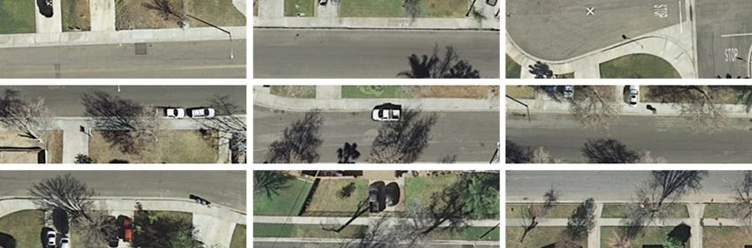
Luo et al                                                                                                              501

                                                              Table 1. Example Network Graphs (from National Center for
                                                              Sustainable Transportation [3])
                                                              a. Example Link Table

                                                              Vnet linkID     Node1ID       Node2ID       Road width (m)

                                                              1                  2586         2601             10
                                                              2                  2601         2617             10
                                                              3                  1822         1932             10
                                                              4                  2085         2176             10
                                                              5                  2070         2085             10
                                                              .                   .            .               .
                                                              Link j            Node1j       Node2j           Widthj

                                                              b. Example Node Table
                                                              Vnet nodeID                 NodeX                   NodeY

Figure 2. Flow chart of overall methodology, adopted from     1                          460188.2                3758112
National Center for Sustainable Transportation (3).           2                          460268.5                3758106
                                                              3                          460323                  3758103
                                                              4                          460331.3                3758089
                                                              5                          460356.3                3758100
network. Geographic processing software was applied,          .                          .                       ...
and all features were projected to universal transverse       Nodei                      Xi                      Yi
mercator (UTM) coordinate system (12, 13). The prepro-
cessing includes the following steps:
                                                                       ‘‘BLVD’’. Based on the suffix of road, a general
   (1) To remove freeways and ramps from the Vnet, as                  road width was assigned to each link. For exam-
       we assume that sidewalks do not exist by the side               ple, roads with AVE, CIR, CT, DR, CN, PL,
       of freeways and freeway ramps.                                  VLG, WAY, TRL, or TER were given a 10-m
   (2) To prevent duplicating sidewalk links, we remove                road width, and roads with BLVD were given an
       one edge and keep only the other consistent edge                18-m width. A number of exceptions were made
       along the road, if one section of arterial is pre-              based on the knowledge of the local streets and
       sented with two edges. For example, for an arter-               survey of Google Maps.
       ial that has an island in the middle and the
       vehicle traffic of two directions are represented
       with two parallel links, only one consistent edge
       will be kept. This step will introduce errors in the
       sweeping step (see Image Sweeping section), and
                                                              Mapping Vnet to Pnet
       potential improvement will be discussed in future      With the preprocessed Vnet, we can now prepare to map
       works.                                                 the preliminary sidewalk nodes. We assume that sidewalk
   (3) To simplify link geometry, the filtered Vnet links     segments are present on both sides of a Vnet link, and
       are generalized (14, 15). This step not only pre-      the sidewalk links are all connected with sidewalk nodes
       serves the geometry of the network but also            in Pnet as in Vnet. As shown in Figure 3a, our goal for
       reduces the number of links by up to 20%.              the mapping from Vnet to Pnet is to calculate the coordi-
   (4) To build the Vnet graph based on the prepro-           nates of four preliminary Pnet nodes (P1, P2, Q1, Q2)
       cessed Vnet shapefile. An example link table and       based on the two Vnet nodes (X1, Y1, X2, Y2) of one
       node table are shown in Table 1.                       roadway link (Linki) and the roadway link’s half-width
   (5) To assign road width and other critical values to      (d, roadway centerline to the edge of sidewalk) which
       roadway links. Detailed information about Vnet         was estimated as described in Equation 5 below.
       road width and number of lanes is not widely              X1, Y1, X2, Y2 are Cartesian coordinates (UTM) of
       available for local streets in California, therefore   the link nodes. To calculate the correct merged sidewalk
       in this study, the road width was estimated based      node that is shown as a blue/orange diamond in
       on the road names provided by NAVTEQ                   Figure 3b, one condition is that we should guarantee that
       Streets (16). The roadway names are recorded           point P1 and P2 always fall into a predictable side (e.g.,
       with the name and the road type, for example,          upper or lower side, left or right side) of their original
       ‘‘Magnolia’’ and ‘‘AVE,’’ ‘‘Van Buren’’ and            Vnet link. In this case, we specify that a Pnet link’s P1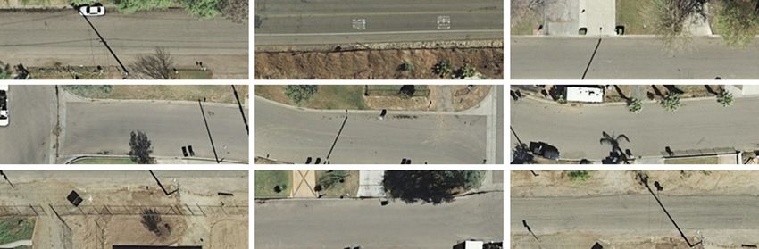
502                                                                                                       Transportation Research Record 2673(8)

Figure 3. Schematics of mapping the preliminary sidewalk nodes (from National Center for Sustainable Transportation [3]).

and P2 must fall within the upper or right-hand side of                             The general method is to iterate through all the nodes
its original Vnet link, as shown in Figure 3a and b. To                          in Vnet. For each Vnet node (e.g., the red star in
control the relative position of P1, P2, Q1, Q2, the fol-                        Figure 3b), we rank all the connected Vnet links by the
lowing steps are applied. When X1 equals X2 and Y1 is                            relative angle to X-axis. Referring to Figure 3c, the four
smaller than Y2, or when X1 is larger than X2, we swap                           links can be ranked as Link1, Link2, Link3, and Link4.
the values of (X1, Y1) with (X2, Y2) to guarantee that                           In Area12, we can locate which Pnet link of Link1 will
the (X1, Y1) is at the left side or at the top of (X2, Y2).                      intersect with the Pnet link of Link2 based on the coordi-
Then the coordinates of P1, P2, Q1, and Q2 are calcu-                            nates and the angle bisector formed between Link1 and
lated by the formulas:                                                           Link2. Then, the intersection coordinates can be com-
                                                                                 puted, and the coordinates of preliminary Pnet nodes
P1x = X1  d=LðY2  Y1Þ, P1y = Y1 + d=LðX2  X1Þ                                 can be updated. The pseudocode for this process in
                                              ð1Þ                                Matlab can be shown as

Q1x = X1 + d=LðY2  Y1Þ, Q1y = Y1  d=LðX2  X1Þ
                                              ð2Þ
                                                                                 function ProcessPreliminaryPnetNodes(VnetGraph);
P2x = X2  d=LðY2  Y1Þ, P2y = Y2 + d=LðX2  X1Þ                                 % calculate the coordinates of Pnet Node (P1,P2,Q1,Q2) for all
                                                                                    Vnet links in the Vnet
                                                                           ð3Þ   initialize Pnet Node based on Equations 1 to 5
                                                                                 Pnet Node = Vnet Link ID, Vnet Node ID, new Pnet LinkID, new
Q2x = X2 + d=LðY2  Y1Þ, Q2y = Y2  d=LðX2  X1Þ                                    Pnet NodeID, P1x, P1y, P2x, P2y, Q1x, Q1y, Q2x, Q2y
                                                                           ð4Þ   for each Vnet Node in VnetGraph
                                                                                    search number of Vnet links n connected with Vnet Node i
where d is the assumed distance from road centerline to                             if n ==1
the edge of the sidewalk; L is the link length. Since all the                          keep Pnet Nodes the same
                                                                                    else
links are processed to be straight segments, L can be cal-                             rank n links by their relative angle to x-axis as shown in
culated as                                                                       Figure 3c
                  qffiffiffiffiffiffiffiffiffiffiffiffiffiffiffiffiffiffiffiffiffiffiffiffiffiffiffiffiffiffiffiffiffiffiffiffiffiffiffiffiffiffiffiffiffiffiffiffiffiffiffiffiffi               for j = 1:n
                                                                                       extract coordinates of (P1,P2,Q1,Q2) for link(j) and
             L=    ðX1  X2Þ2 + ðY1  Y2Þ2                                 ð5Þ   (P1,P2,Q1,Q2) for link(j + 1)
                                                                                       search the area between link(j) and link(j + 1)
Next, we need to process the preliminary sidewalk links                                locate the intersection of Pnet of link(j) and Pnet of
at intersections. As shown in Figure 3b, when two Vnet                           link(j + 1) based on coordinates of (P1,P2,Q1,Q2)
                                                                                       calculate the coordinates of Pnet intersection: interX, interY
links intersect at a Vnet node (marked by a red star), the
                                                                                       mark the intersection point as jth crossing point for
newly generated Pnet links (by following previous rules)                         crosswalk generation
as shown in purple and green broken lines, will also inter-                            update the Pnet ID of the intersected P or Q point to be the
sect. We aim at calculating the ‘‘merged sidewalk node’’                         same
(marked in blue and orange diamonds) based on the Pnet                                 update the coordinates of the intersected P or Q points with
                                                                                 interX, and interY
nodes, which also form the intersection nodes at street                          return Pnet Node
crossings.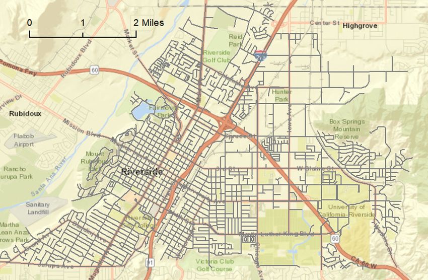
Luo et al 503
Image Sweeping
To collect images that can be trained by a machine learn-
ing algorithm, we considered capturing a uniform size of
images which contain desired objects to be recognized by
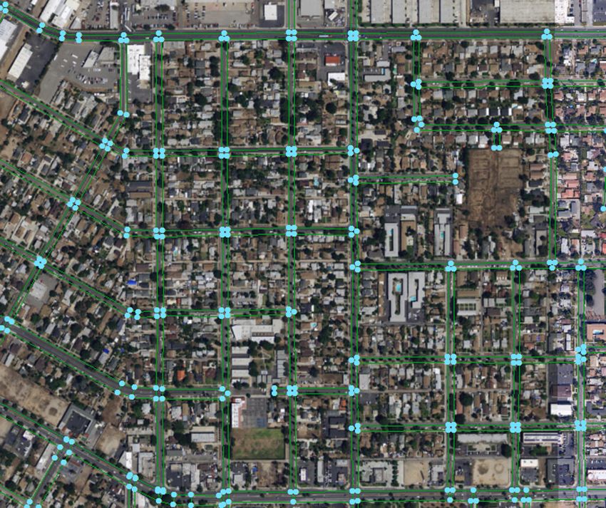
the algorithm. As shown in Figure 4, collecting images
along the Pnet links involves a large number of screen-
shot operations and it would be challenging to manually
perform the task.
With the aid of ArcPy package (17), we developed a
Python script and executed it in ArcMap-Python
Environment. The Python script was able to command
the map interface to zoom into each Pnet link at a desig-
nated map scale (1:300 in this study) and take screen-
shots at ESRI World Imagery Basemap with designated
image size (e.g., 200 3 400 pixel). The pseudocode is
provided below. For alternative imagery sources (e.g.,
drones), we recommend a minimum resolution of 1:500
scale and should be orthorectified and aligned with the
Figure 4. An example of mapped sidewalk based on vehicle digital road network.
roadway network (from National Center for Sustainable
Transportation [3]).
function SweepingImage(PnetGraph):
import arcpy, arcpy.mapping, pyautogui, numpy
If we assume there is a total of J links (link1, link2,
set map scale, image size and other paramters
., linkj) in Vnet Graph, then the mapping method will for each Pnet Link in PnetGraph:
yield 4J preliminary sidewalk nodes, and 2J preliminary extract the two Pnet node coordinates (Px1, Py1, Px2, Py2) of
sidewalk links. Next, we assume there are m nodes in the the Pnet Link
Vnet, among which x out of m nodes are connected with calculate the angle between the Pnet link and x positive axis
based on (Px1, Py1, Px2, Py2)
only one link, and the other (m–x) links are connected rotate the map frame with respect to the angle to position the
with j links (n ø 2). Then after the execution of the pseu- link parallel to x axis
docode above, theP total number of Pnet sidewalk nodes pan the map frame at the designated scale and center the Pnet
will become 2x + j. Link
mx calculate the screen pixel location based on the screen
An example output of the pseudocode above is illu- resolution, screen size, and the Pnet Link location
strated in Figure 4, where the preliminary sidewalks are screenshot and save an image of the designated size
shown in green line, and sidewalk nodes are shown in
blue dots.
Even though the script has reduced manual operation
time, it is a rather time-consuming process in this study.
Development of Image Processing For example, with a desktop computer of Intel Core i3-
Algorithm Based on Machine Learning 2120 CPU (@3.3GHz, 8 GB RAM), capturing 1,000
With the initialized sidewalk network, our next goal is to screenshots will take approximately 88 min.
identify whether a certain segment is concrete or not.
When viewing the aerial images of the street at a
zoomed-in level, most unobstructed paved and missing Image Labeling
sidewalk sections can be easily identified with human After collecting a large number of aerial images along the
eyes, as shown in Figures 5 and 6. To enable a large initial sidewalk network (i.e., Pnet), we labeled a subset
number of image collection, we developed an image of them for training the proposed machine learning algo-
sweeping method to capture the aerial images along the rithm. In this study, labeling images means that we assign
Pnet. After collecting and labeling a considerable num- a category for a group of images which share similar
ber of images, a CNN, which is one of the machine attributes. Specifically, as shown in Figure 5, a label of
learning methods, is applied to train the learning algo- ‘‘paved present’’ is assigned to a group of images which
rithm to identify the ‘‘sidewalk surface’’ feature. clearly present concrete-surfaced sidewalk segments. On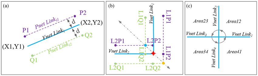
504                                                                                             Transportation Research Record 2673(8)

Figure 5. Screenshots of ‘‘paved present’’ sidewalk sections from aerial image at 1 to 300 scale (from National Center for Sustainable
Transportation [3]).

Figure 6. Screenshots of ‘‘missing’’ sidewalk sections from aerial image at 1 to 300 scale (from National Center for Sustainable
Transportation [3]).

the other hand, in Figure 6, the label of ‘‘missing side-              green, and blue [RGB]) of each pixel in the image. For
walk’’ is assigned to a group of images which can be iden-             example, if one image is of size 200 3 400 pixels, the
tified as a lack of paved sidewalk segments.                           image will be represented with a 200 3 400 3 3 matrix.
    Generally, the more labeled images there are, the better           At the same time, this matrix will be associated with a
the training results will be. Usually, image classification            label, in this case, ‘‘1’’ for sidewalk present or ‘‘2’’ for
requires a large number of training samples. The labeled               missing sidewalk. As shown in Figure 7, the input to the
images will be critical inputs for the next training step.             network is the labeled 3-channel RGB image, and the
                                                                       output is a 2-entry vector indicating the probability of
                                                                       whether the image belongs to case 1, with [1,0] as label,
Training Machine Learning Parameters
                                                                       or case 2, with [0,1] as label. The network loss is defined
The model used for training the parameters is a CNN                    as a cross-entropy loss:
(18, 19), with architecture shown in the figure below. It is
                                                                                                       X
assumed that for each layer the batch size equals 1. The                                      L=            yi logxi                    ð6Þ
CNN structure was chosen because CNN is known for                                                        i
outstanding performance in the realm of image
classification.                                                        With xi and yi as the entry of label and network output,
   An image is usually represented with a vector of val-               respectively. The network consists of multiple convolu-
ues, which corresponds to the value of color (e.g., red,               tional layers (conv), with a kernel size of 3 3 3 and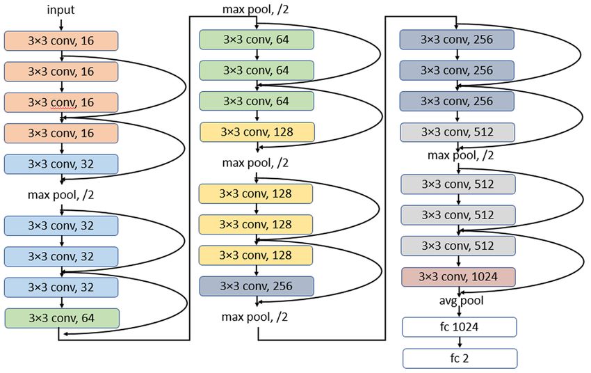
Luo et al                                                                                                                  505

Figure 7. Flowchart of CNN applied in the learning algorithm
                                                               Figure 8. Example roadway network in the case study (from
(adopted from He et al. (19) with descriptions below).
                                                               National Center for Sustainable Transportation [3]).

stride equals 1, followed by rectified linear unit (ReLU)      paved and 840 missing) were used as training dataset,
as nonlinear activation function. Residual blocks which        180 images (80 paved and 100 missing) for validation,
add padded input of one layer to the output of next layer      and 180 images (80 paved and 100 missing) for testing.
are used to increase the training speed of the network         All images were chosen randomly from the labeled
(19). The learnable parameters include filters, weights,       images.
and biases in the convolutional layers and fully con-
nected layers (fc) are updated using an adaptive moment        Training Results
estimation (Adam) (20) optimizer with a learning rate of
1 3 10–4.                                                      Following the training of a deep CNN, we blind-tested
                                                               its prediction performance by feeding it with the labeled
                                                               images in a new test set. The training results are shown in
Case Study and Performance Evaluation                          Table 2. The results demonstrated that the learning algo-
                                                               rithm is able to identify the two categories of sidewalk
Preprocessing and Initial Mapping
                                                               using the presented framework at a total prediction rate
For a case study, we selected an area surrounding              of 97.2%. Table 2 also listed the prediction performance
University of California, Riverside shown in Figure 8.         of a simple logistic regression (LR) method applied in the
There are 4,385 roadway links in the Vnet. The prepro-         previous related research (3). It is evident that CNN algo-
cessing and initial mapping were performed by following        rithm has significantly higher prediction rate than the LR
the methods described earlier. The initial mapping cre-        algorithm.
ated 14,806 sidewalk links, including 386 cul-de-sac,              Furthermore, with the learning algorithm, we classi-
8,388 sidewalk segments, and 6,032 crosswalks. The initi-      fied all the images that were collected from the sweeping
alized sidewalk map can be viewed at https://arcg.is/          method. Then 1,041 new images (aside from the training,
184PbK.                                                        validation, and test sets) were labeled manually to vali-
                                                               date the predication results of the learning algorithm.
                                                               We found that 964 images were correctly classified. The
Sweeping and Labeling Images                                   results indicated that our learning algorithm can achieve
In this project, image sweeping and labeling are the most      a satisfactory prediction rate of 92.6% in the blind test.
time-consuming processes. There are 8,388 sidewalk seg-            The CNN is implemented in TensorFlow (21). In rela-
ments and their aerial images need to be captured (cross-      tion to computation performance, the training process
walks are not swept because crosswalks are usually a           took approximately 20 min with 8,000 iterations, corre-
part of vehicle roadways). Sweeping 8,388 images took          sponding to about 54 epochs. The convergence plot is
approximately 12 h.                                            shown in Figure 9, indicating that convergence was
   We marked 792 images with ‘‘paved’’ label and 1040          achieved with approximately 8,000 iterations. The train-
images with ‘‘missing’’ label. Each image captured an          ing, validation, and testing of the network were per-
area 50 3 16 m and was of size 603 3 192 pixels.               formed on a PC with four-core 3.60 GHz CPU, 16GB of
Among the 1,832 labeled images, 1,472 images (632              RAM, and Nvidia GeForce GTX 1080Ti GPU.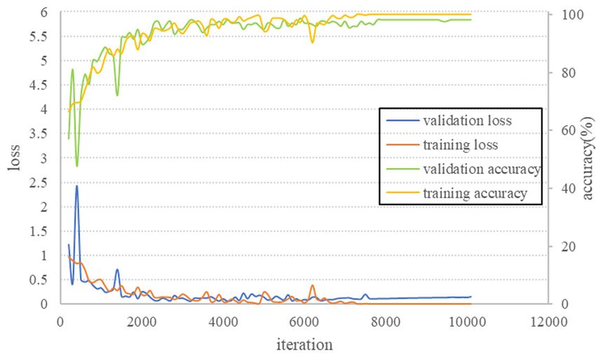
506                                                                                              Transportation Research Record 2673(8)

Table 2. Training Result

Number of images                                 Case 1 (‘‘present’’)                      Case 2 (‘‘missing’’)                   Total

Training sample                                  632                                       840                                   1472
Validation sample                                80                                        100                                   180
Testing sample                                   80                                        100                                   180
Testing positive: CNN                            77                                        98                                    175
Testing negative: CNN                            3                                         2                                     5
Testing prediction rate: CNN                     96.3%                                     98%                                   97.2%
Testing positive: LR                             41                                        66                                    107
Testing negative: LR                             39                                        34                                    73
Testing prediction rate: LR                      51.3%                                     66%                                   59.4%

                                                                           2.   Reduce the image size and focus on increasing
                                                                                the number of labeled images. In the case study,
                                                                                the images were captured at a scale of 1:300 and
                                                                                it resulted in a large image with 115,776 pixels.
                                                                                However, the number of labeled images is more
                                                                                important than the size of the image. We think
                                                                                the following measures are worth trying to fur-
                                                                                ther increase the prediction rate: 1) try a map
                                                                                scale of 1:400, 2) reduce the section length from
                                                                                50 m to 30 m, and 3) increase the number of
                                                                                labeled images to 2,000.
                                                                           3.   Try to classify the captured images into more
                                                                                detailed categories, rather than only two cate-
                                                                                gories. For example, green space, curb cut, park-
Figure 9. Convergence plot of the training process.                             ing lot/driveway. Also, there are many obstructed
                                                                                images (e.g., sidewalk shaded by trees, shadows,
                                                                                or unable to identify objects) in the collected
Discussion and Future Directions                                                image set and those images should be identified
                                                                                as well.
In this study, we proposed a method that takes full
advantage of available data sources and builds on top of
the existing roadway network to create a digital sidewalk               Acknowledgments
inventory. The learning algorithm is able to achieve a                  We would like to acknowledge our funding agencies. The work
satisfactory prediction rate of 92.6% in the blind test,                was sponsored by U.S. Department of Transportation Grant
especially, it can successfully identify areas with poor                No. DTRT13-G-UTC29, and California Department of
sidewalk conditions as shown in Figure 6. The mapping                   Transportation Contract No. 65A0527. We thank Mr.
approach could potentially lay the foundation for side-                 Alexander Vu from the Center for Environmental Research
                                                                        and Technology for his technical support. We greatly appreci-
walk inventory and improved active traveler applica-
                                                                        ate Mr. Nathan Mustafa from City of Riverside and Mr.
tions. What is more important is that there is potential                Dustin Foster from Caltrans for their valuable inputs. Last but
for future improvement:                                                 not least, we would like to thank our project manager Mr.
                                                                        Patrick Tyner and Ms. Lauren Iacobucci for their support
   1.   Improve the preprocessing methods and the Pnet                  throughout the project.
        initialization process. For example, arterials with
        two road edges could be merged into one link to                 Author Contributions
        capture the correct centerline location. The road
                                                                        The authors confirm contribution to the paper as follows: study
        width could be interpolated based on city-wide
                                                                        conception and design: JL and GW; data collection: JL and
        roadway classification or image processing tech-                GW; analysis and interpretation of results: JL, GW, and ZW;
        niques such as edge detection.                                  draft manuscript preparation: JL, GW, ZW, KB, and MB. All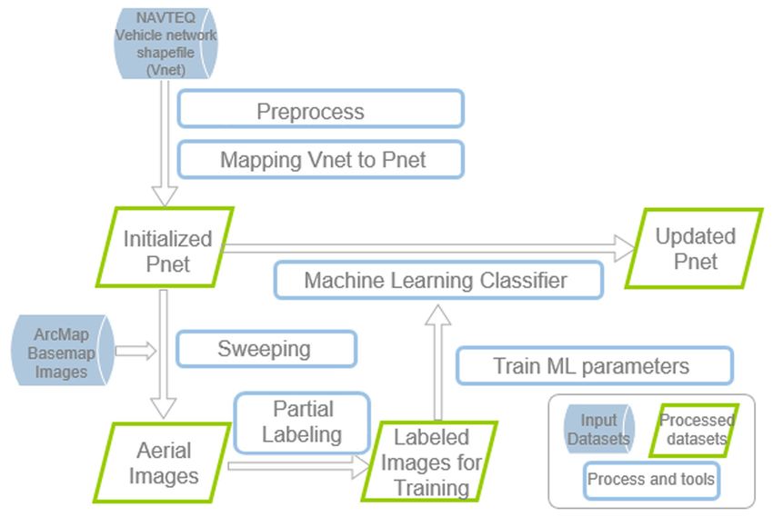
Luo et al                                                                                                                       507

authors reviewed the results and approved the final version of        9. He, K., X. Zhang, S. Ren, and J. Sun. Delving Deep into
the manuscript.                                                          Rectifiers: Surpassing Human-Level Performance on Ima-
                                                                         genet Classification. Proc., IEEE International Conference
                                                                         on Computer Vision, 2015, pp. 1026–1034.
References
                                                                     10. California Department of Transportation. Chapter 100:
 1. Ehrenfeucht, R., and A. Loukaitou-Sideris. Planning                  Basic Design Policies, Highway Design Manual. 2015.
    Urban Sidewalks: Infrastructure, Daily Life and Destina-             http://www.dot.ca.gov/design/manuals/hdm/chp0100.pdf.
    tions. Journal of Urban Design, Vol. 15, No. 4, 2010,                Accessed March 1, 2019.
    pp. 459–471.                                                     11. Environmental Systems Research Institute. Shapefile Tech-
 2. Hanson, S., and A. Jones. Is there Evidence that Walking             nical Description. http://www.esri.com/library/whitepapers/
    Groups Have Health Benefits? A Systematic Review and                 pdfs/shapefile.pdf. Accessed March 1, 2019.
    Meta-Analysis. British Journal of Sports Medicine, Vol. 49,      12. Environmental Systems Research Institute. Project.
    No. 11, 2015, pp. 710–715.                                           http://desktop.arcgis.com/en/arcmap/10.3/tools/cove
 3. National Center for Sustainable Transportation. Develop-             rage-toolbox/project.htm. Accessed March 1, 2019.
    ing an Interactive Machine-learning-Based Approach for           13. ESRI ArcGIS for Desktop. Universal Transverse Mercator
    Sidewalk Digitalization. 2018. https://ncst.ucdavis.edu/             Coordinate System. http://desktop.arcgis.com/en/arcmap/
    project/developing-an-interactive-machine-learning-based-            10.3/guide-books/map-projections/universal-transverse-
    approach-for-sidewalk-digitalization/. Accessed March 1,             mercator.htm. Accessed March 1, 2019.
    2019.                                                            14. ESRI ArcGIS for Desktop. Generalize. http://desktop.
 4. Champaign Urbana Urbanized Area Transportation                       arcgis.com/en/arcmap/10.3/tools/editing-toolbox/gener
    Study. Sidewalk Network Inventory and Assessment – for               alize.htm. Accessed March 1, 2019.
    the Champaign Urban Urbanized Area. Illinois Department          15. ESRI ArcGIS for Desktop. Methods for Splitting Line
    of Transportation, Ill., 2016.                                       Features. http://desktop.arcgis.com/en/arcmap/10.3/mana
 5. Frackelton, A., A. Grossman, E. Palinginis, F. Castrillon,           ge-data/editing-existing-features/ways-to-split-a-line-featu
    V. Elango, and R. Guensler. Measuring Walkability: Devel-            re.htm#ESRI_SECTION1_84606E86D9DE4FA5A95AEB
    opment of an Automated Sidewalk Quality Assessment                   C095657767. Accessed March 1, 2019.
    Tool. Suburban Sustainability, Vol. 1, No. 1, 2013, p. 4.        16. NAVTEQ. NAVSTREETS Street Data Reference Manual
 6. CitiLab. Citilabs’ Streetlytics Provides Complete Hour-by-           v4.4. 2012.
    Hour Pedestrian Volume Analytics for the Entire United States.   17. ESRI ArcGIS Pro. ArcPy Reference. http://pro.arcgis.com/
    http://www.citilabs.com/citilabs_blog/citilabs-leverages-loca        en/pro-app/arcpy/main/arcgis-pro-arcpy-reference.htm.
    tion-data-create-first-ever-nationwide-analytics-platform-pede       Accessed March 1, 2019.
    strian-movements/?utm_campaign=Company%20News&                   18. LeCun, Y., Y. Bengio, and G. Hinton. Deep Learning.
    utm_source=hs_email&utm_medium=email&utm_content                     Nature, Vol. 521, No. 7553, 2015, p. 436.
    =62537380&_hsenc=p2ANqtz-8sefRcesPCVz4C1UlOAjjwv                 19. He, K., X. Zhang, S. Ren, and J. Sun. Deep Residual
    bJUFiQdqyPx9SQk9BFgR0uUgGQ0inYlZIQRauzFywegd                         Learning for Image Recognition. Proc., IEEE Conference
    6X_DJZzDfslfkmzSaKNwFxvkQ&_hsmi=62537380.                            on Computer Vision and Pattern Recognition, 2016,
    Accessed March 1, 2019.                                              pp. 770–778.
 7. Bao, J., T. He, S. Ruan, Y. Li, and Y. Zheng. Planning           20. Kingma, D. P., and J. Ba. Adam: A Method for Stochastic
    Bike Lanes Based on Sharing-Bikes’ Trajectories. Proc.,              Optimization. arXiv preprint arXiv:1412.6980, 2014.
    23rd ACM SIGKDD International Conference on                      21. Abadi, M., P. Barham, J. Chen, Z. Chen, A. Davis, J.
    Knowledge Discovery and Data Mining, ACM, 2017,                      Dean, M. Devin, S. Ghemawat, G. Irving, and M. Isard.
    pp. 1377–1386.                                                       Tensorflow: A System for Large-Scale Machine Learning.
 8. Bolten, N., A. Amini, Y. Hao, V. Ravichandran, A. Ste-               Symposium on Operating Systems Design and Implementa-
    phens, and A. Caspi. Urban Sidewalks: Visualization and              tion, No. 16, 2016. pp. 265–283.
    Routing for Individuals with Limited Mobility. Proc., 1st
    International ACM SIGSPATIAL Workshop on Smart Cit-              The Standing Committee on Information Systems               and
    ies and Urban Analytics, ACM, 2015, pp. 122–125.                 Technology (ABJ50) peer-reviewed this paper (19-02287).
You can also read