ACTIVE FAULT TOLERANCE CONTROL BASED ON CONSISTENT MATRIX FOR MULTIMOTOR SYNCHRONOUS SYSTEM - GOOA

Hindawi
Complexity
Volume 2020, Article ID 1426193, 11 pages
https://doi.org/10.1155/2020/1426193

Research Article
Active Fault Tolerance Control Based on Consistent Matrix for
Multimotor Synchronous System

 Haijie Mao ,1,2,3 Wei Li ,1,2,3 Xiaolin Feng ,1,2,3 and Haochuan Zhang1
 1
 College of Electrical and Information Engineering, Lanzhou University of Technology, Lanzhou 730050, China
 2
 Key Laboratory of Gansu Advanced Control for Industrial Processes, Lanzhou 730050, China
 3
 National Demonstration Center for Experimental Electrical and Control Engineering Education,
 Lanzhou University of Technology, Lanzhou 730050, China

 Correspondence should be addressed to Xiaolin Feng; splendor2003@126.com

 Received 9 November 2019; Revised 18 January 2020; Accepted 5 February 2020; Published 21 April 2020

 Academic Editor: Xianming Zhang

 Copyright © 2020 Haijie Mao et al. This is an open access article distributed under the Creative Commons Attribution License,
 which permits unrestricted use, distribution, and reproduction in any medium, provided the original work is properly cited.

 This paper presents an active fault-tolerant method to mitigate sensor failures in multimotor synchronous control. First, inspired
 by the construction of the coupling matrix in complex network synchronous output, a consistent matrix is designed based on
 structural redundancy in synchronous control. This consistent matrix has two advantages: one is that it can reflect different sensor
 output similarities and the other one is that it can detect, locate, and estimate the sensor fault. Then, the fault information is
 integrated into the design of tolerance control with an improved mean feedback mechanism. The proposed method is suitable for
 both single and multiple fault situations, and its effectiveness is finally verified by both MATLAB simulation and the ABB
 semiphysical experimental platform.

1. Introduction faults in motion control systems for decades [8–15]. They
 can be roughly divided into two categories, namely,
Due to great load drive capabilities and more flexible motion mathematical model-based and data-driven-based [9]. The
modes, multimotor synchronous driven systems have been core of the mathematical model method is the design of
widely applied in numerous industry domains including various types of observers. For example, Mao et al. [10]
robotics, paper making, and belt conveyors [1–4]. The ob- adopted adaptive disturbance rejection control (ADRC) and
jective of synchronous control is to ensure synchronization an extended state observer (ESO) to estimate the speed in a
of speed or displacement between different motors under current loop, which realized FTC for a speed sensor fault and
different loads or disturbances [5–7]. In multimotor syn- improved the multimotor synchronization accuracy. Naja-
chronous control systems, the sensors used to measure speed fabadi et al. [11] solved the problem of diagnosing and
or position are easily malfunctioned due to ageing, collision, isolating three sensor faults for current, voltage, and speed in
or electromagnetic interference. Once a fault occurs, the induction motors through designing an adaptive current
synchronization control performance will be seriously af- observer for rotor resistance estimation. For a speed sensor
fected and disastrous consequences may happen. Therefore, failure in an induction motor, Marino et al. [12] designed an
identifying such faults and taking effective measures in time adaptive observer to detect sensor faults online, and fault
is of great significance for ensuring system safety, reliability, tolerance was realized based on indirect magnetic field
and product quality [5, 6]. orientation control. In recent years, aiming at the difficulty
 The development of fault detection and diagnosis (FDD) of modelling, the data-driven method has gradually become
and fault-tolerant control (FTC) based on analytical re- a new research hot spot, which has received extensive at-
dundancy provides strong support for ensuring the security tention [13–15]. Based on the large amount of online and
of the system. Many researchers have studied FTC for sensor offline monitoring data existing in the system, this method

2 Complexity

can characterize the normal and fault modes in the system paper focuses on fault diagnosis and tolerance in multimotor
based on that useful information hidden in data using data synchronous control systems, the deviation-coupled syn-
mining and processing technologies. Consequently, it has chronous control structure in [10] is adopted. The control
been recognized as a practical diagnostic technology. As an principle is shown in Figure 1, where ADRC is a kind of
application, by collecting line voltage and performing fast controller and S.C. is the synchronous compensator or
Fourier transform, a data-driven method using a two-layer controller, such as PI or PID.
Bayesian network was proposed in [13] to obtain fault
characteristics. As a result, fault diagnosis of an inverter in 3. Sensor Fault FDD and FTC Design Based on
PMSM was realized.
 Complex Network Consistent Matrix
 Recalling the existing results in the literature, most re-
sults are directed to single-motor drives. Although some of 3.1. Establishment of Complex Dynamical Network
them are also applicable to multimotor synchronous driving Consistent Matrix
modes, they still have some limitations since the presented
algorithms are complicated and difficult to implement. To 3.1.1. Complex Network Coupling Matrix. Based on graph
overcome such limitations, in this paper, through exploring theory, a complex network system with identical dynamic
mathematical model-based and data-driven-based methods’ systems as nodes that satisfies the dissipation conditions can
characters and shortages, we devise a combination method be described as follows [28]:
based on a complex network. N
 The complex network model has been widely used in x_ i � f xi (t) + σ aij H xj (t) , (1)
many fields, such as power grids and aerospace [16–19]. A j�1
typical complex network system consists of a number of
subsystems that are usually coupled with each other. Typ- where xi � (xi1 , xi2 , . . . , xiN )T ∈ Rn is the state of node i,
ically, a multimotor synchronous control system is such a i � 1, 2, . . . , N; f ∈ C[Rn , Rn ] is a known function (often a
complex network. The consistency study of complex net- nonlinear function); σ > 0 is the coupling strength of the
works, that is, complex network synchronization control, is network; A � (aij )N×N is the coupling matrix of the network,
an important research topic in the field of complex networks. which satisfies j aij � 0, i � 1, 2, . . . , N; and H ∈ C[Rn , Rn ],
 Redundancy is the basis of fault diagnosis and fault which is a coupling function.
tolerance. In this paper, inspired by the construction of a The coupling matrix A can be used to describe an un-
coupling matrix in complex network systems, a consistent directed topology. If there is a connection between node
matrix is designed to characterize the similarities of output i and node j, then aij � aji � k, k > 0, otherwise
data of different sensors, using the structure and information aij � aji � 0, i ≠ j. The diagonal elements of matrix A satisfy
redundancy in multimotor synchronous control systems. N N
Based on online analysis and judgment of matrix elements aii � − aij � − aji . (2)
 j�1,j≠i j�1,j≠i
and eigenvalues, the detection, location, and estimation for
faulty sensors are realized. As a result, a novel improved
mean feedback strategy is presented using structural re-
dundancy and fault information to achieve fault tolerance. It Definition 1. In the dynamic network (1), the network is said
is shown through simulation and experiment that system to be consecutively synchronized for any initial conditions
security and reliability are greatly improved. [29] if
 �� ��
 lim ���xi (t) − xj (t)��� � 0, i, j � 1, 2, . . . , N. (3)
 t⟶∞
2. Deviation-Coupled Synchronous
 Control Structure The coupling matrix A determined by the complex
 network structure reflects the synchronous state or con-
The research on multimotor synchronous control strategies sistent attribute of the network. Inspired by the nature of the
mainly includes two aspects, synchronous control structure coupling matrix, this paper constructs a consistent matrix
and synchronous control algorithm. In terms of the control with the abovementioned properties to characterize the
structure, there are mainly serial master-slave control [20], synchronization or consistency of a complex network. When
virtual spindle control [21], cross-coupling control [22, 23], the system is in an abnormal state due to faults, the con-
and deviation-coupling control [24]. Among them, devia- sistency will be destroyed, and the resulting abnormality will
tion coupling adopts the compensation control strategy and also be reflected in the coupling matrix. So, with the location
the comprehensive effect is more positive than others in and size of the matrix element that changes, the fault can be
aspects of starting characteristics, disturbance suppression detected and located.
ability, applicable range, and convenience of engineering
realization. Accordingly, its practical applications have been
found in a wider range of fields. In terms of control algo- 3.1.2. Data-Driven Consistent Matrix Construction.
rithms, which are mainly for load uncertainty and unknown Figure 1 shows that multimotor synchronous control is a
interference, various robust control algorithms are devised typical complex network system. Considering the control
[10, 24–27], such as sliding mode control, internal model objectives, this paper pays more attention to judging the
control, and active disturbance rejection control. Since this consistency of the complex network output. To evaluate the

Complexity 3

 y∗ y1 Remark 2. For the network synchronization, the abnormal
 ADRC Motor 1 Sensor 1 or fault output of a certain node will be far away from the
 output of other normal nodes. It will decrease the consis-
 S.C. tency between them accordingly. This change can be directly
 reflected from the corresponding position in the matrix,
 y2 which is the basis for follow-up fault diagnosis studies.
 ADRC Motor 2 Sensor 2

 S.C.
 3.2. Sensor Fault Diagnosis Based on Consistent Matrix
 3.2.1. Consistent Matrix Analysis under Normal/Fault
 Condition of the Sensor. Based on the design of the con-
 yN
 ADRC Motor n Sensor n sistent matrix described above, for a multimotor synchro-
 nous control system shown in Figure 1, the following
 S.C. assumptions are made.

 Assumption 1. There are N motors to be synchronized, and
 Average the output of each subsystem can be regarded as a node of a
 complex network.
Figure 1: Deviation-coupling synchronization control structure.
 Assumption 2. The system has good synchronous control
consistency or similarity between different nodes in a performance under normal conditions. The system reaches
complex network, a consistent matrix, which is derived from steady state and has good synchronization accuracy, which
the coupling matrix, is introduced. The process of con- means that yi ≈ yj .
structing the consistent matrix can be summarized as
follows. Assumption 3. When two or more sensors fail at the same
 The output of the N nodes of the multimotor syn- time, the sizes or magnitudes of faults are different.
chronous complex network system shown in Figure 1 is Under the previous assumptions, we can obtain aij ≈ 1
measured by N sensors and constitutes a set and aii ≈ − (N − 1). The eigenvalues of A satisfy λ1 � λ2 �
Y � [y1 , y2 , . . . , yN ]. The consistency between yi and yj is · · · � λN− 1 � − N and λN � 0. When a sensor (taking the ith
represented by the coefficient aij . As aij gets larger, yj and yi sensor as an example) fails, its output will inevitably deviate
become more consistent. The consistency between two from other normal sensor outputs. The elements in the ith
different nodes is the same, which means aij � aji . Thus, the row and the ith column of A will show ai∗ < 1, a∗i < 1 (except
matrix A is a symmetric matrix. Constructing A is very for the diagonal), and with the magnitude of the fault in-
important to effectively distinguish the consistency between creases, ai∗ ≪ 1, a∗i ≪ 1. The eigenvalues of matrix A will
yi and yj . Generally, it is set as an exponential function of also change accordingly.
the distance between yi and yj . The construction form is
given as follows:
 ���������� 3.2.2. Fault Detection and Location Based on Consistent
 ⎪
 ⎧
 ⎪ − yi (k)− yj (k) 
 2
 Matrix Judgement. From the analysis above on different
 ⎪
 ⎪ a � e , i ≠ j,
 ⎨ ij characteristics of the consistent matrix A before and after the
 A(k) � ⎪ N
 (4) fault, fault detection can be performed by judging the ele-
 ⎪
 ⎪
 ⎪
 ⎩ aii � − aij , i � j, ment size of A. Generally, three types of fault detection
 j�1,i≠j
 methods can be selected:
where yi (k) is the output data from the sensor on node i at (1) A(k) is compared with A(k − l). Taking the length of
sampling moment k, i, j � 1, 2, . . . , N. Matrix A satisfies the the data as l, generate A(k − 1), . . . , A(k − l) and
conditions of the coupling matrix, that is, aij � aji > 0, i ≠ j, compare A(k) with the elements at the corre-
rank(A) � N − 1. It also has the same properties as the sponding position of A(k − l). When a row or col-
coupling matrix. umn of elements in the deviation matrix exceeds the
 predefined threshold, the fault can be detected and
Remark 1. The matrix is completely generated by the output the fault sensor can be located according to the row
data of the sensor, so it can be considered as data-driven or column position of the element exceeding the
based. At the same time, the structure of A reflects the threshold.
distance relationship between two different sensor outputs. (2) Elements in A(k) are compared with 1. With the
Therefore, it has the characteristics of a model. Moreover, analysis above, when the sensor is normal, aij ≈ 1.
the design of A can be considered as a combination of data- When the ith sensor fails, the ith row and the ith
driven and model-based methods, which has the advantages column elements in A(k) appear to be much smaller
of convenient data acquisition and reflecting the mechanism than 1, ai∗ < 1, a∗i < 1. The fault sensor can be
characteristics of the network model. identified and located accordingly.

4 Complexity

 (3) Using the change in A(k) eigenvalues. The eigen- It is worth mentioning that the diagnostic method above
 values of the consistent matrix are also changed is also applicable to multiple fault situations. It means that
 when a fault occurs. The normal eigenvalues are when multiple sensors fail simultaneously, multirow and
 approximately − N and 0. After the fault occurs, the multicolumn element values will satisfy aij < 1 at the cor-
 matrix A(k) still satisfies the dissipation character- responding positions in the matrix.
 istics, although rank(A) � N − 1, except for the ei- For example, when M sensors fault simultaneously in a
 genvalue 0, the distribution of other eigenvalues will multimotor synchronous control system composed of N
 change instead. Motors (M < N) under Assumption 3, there will be C2N− M �
 (N − M)(N − M − 1)/2 element values satisfying aij � 1,
 For the abovementioned three methods, from the
 while other M(2N − M − 1)/2 elements will satisfy aij < 1,
perspective of detection speed and reliability, there are
 except for diagonal elements. The diagnostic process is
different characteristics. Method (1) uses l sample data to
 similar to the single fault scenario.
test. With the sample number increasing, the reliability of
 However, as the number of faulty sensors increases,
the detection is improved, while a certain delay will occur.
 the types of faults diversify and the number of elements to
Therefore, from real-time and reliability consideration, l
 be judged will increase greatly. Accordingly, the diagnosis
should not be too large. Method (2) has fast diagnostic
 time is prolonged. At the same time, the distances be-
speed and good real-time performance, but the anti-in-
 tween two different sensors, especially between the faulty
terference performance is poor, possibly leading to false
 sensors, are various. All of these will decrease the overall
alarms. Method (3) is essentially the same as Method (2).
 diagnostic reliability of the method to some extent, es-
They both are based on A(k)′ s own elements or eigen-
 pecially when the detection threshold is set to a certain
values. However, the limitation of Method (3) lies in that it
 fixed value.
cannot locate the fault.
 Combining the characteristics analysis of the above-
mentioned three methods, to improve the efficiency and 3.2.3. Fault Estimation Based on Eigenvalues of the Consistent
reliability of the diagnosis, it is a good idea to combine Matrix. In addition to detecting and locating the fault,
Methods (1) and (2). When the diagnosis program is the fault size can be estimated by further studying the
implemented, Method (2) is mainly used. After the fault is performance of matrix A. The specific process is as
judged, the A(k) comparison is made with the latter steps in follows.
combination. That is, Method (1) is used for further con- When the ith sensor fails, the consistent matrix A can be
firmation. Diagnosis speed, reliability, and computing re- approximated as (ignoring the noise and synchronization
sources can be simultaneously ensured. error)

 − (N − 2 + β) 1 ··· β ··· 1
 ⎢
 ⎡
 ⎢
 ⎢ ⎤⎥⎥⎥
 ⎢
 ⎢
 ⎢ 1 − (N − 2 + β) · · · β ··· 1 ⎥⎥⎥
 ⎢
 ⎢
 ⎢ ⎥⎥⎥
 ⎢
 ⎢
 ⎢ ⎥⎥⎥
 ⎢
 ⎢ ⋮ ⋮ ⋮ ⋮ ⋮ ⋮ ⎥⎥⎥
 A ≈⎢
 f ⎢
 ⎢
 ⎢
 ⎢ ⎥⎥⎥⎥, (5)
 ⎢
 ⎢
 ⎢ β β · · · − (N − 1)β · · · β ⎥⎥⎥
 ⎢
 ⎢
 ⎢ ⎥⎥⎥
 ⎢
 ⎢
 ⎢ ⎥⎥⎥
 ⎢
 ⎢
 ⎣ ⋮ ⋮ ⋮ ⋮ ⋮ ⋮ ⎥⎥⎦
 1 1 ··· β · · · − (N − 2 + β)

where β is the consistent coefficient between the fault sensor the abovementioned matrix can be transformed into the
and other normal sensors, β < 1. To estimate the fault size, following form:

 − (N − 2 + β) 1 ··· β ··· 1
 ⎢
 ⎡
 ⎢
 ⎢ ⎤⎥⎥⎥
 ⎢
 ⎢
 ⎢ 1 − (N − 1) · · · 1 ··· 1 ⎥⎥⎥
 ⎢
 ⎢
 ⎢ ⎥⎥⎥
 ⎢
 ⎢
 ⎢ ⎥⎥⎥
 ⎢
 ⎢ ⋮ ⋮ ⋮ ⋮ ⋮ ⋮ ⎥⎥⎥
 ≈⎢
 ∗
 Af ⎢
 ⎢
 ⎢ ⎥⎥⎥. (6)
 ⎢
 ⎢
 ⎢ β 1 · · · − (N − 2 + β) · · · 1 ⎥⎥⎥
 ⎢
 ⎢
 ⎢ ⎥⎥⎥
 ⎢
 ⎢
 ⎢ ⎥⎥⎥
 ⎢
 ⎢
 ⎢ ⋮ ⋮ ⋮ ⋮ ⋮ ⋮ ⎥⎥⎥
 ⎣ ⎦
 1 1 ··· 1 · · · − (N − 1)

Complexity 5

 That is, except for a1i � ai1 � β, the diagonal elements is automatically isolated. As a result, fault sensor isolation
remain unchanged from the original rule and the elements in and system fault tolerance can be realized. It does not affect
other positions are all set to 1. It is easy to obtain the ei- the generation of the mean signal, nor does it change the
 ∗
genvalues of Af , which are λ1 � · · · � λN− 2 � − N, topology of the original network.
λN− 1 � − (N − 2 + 2β), and λN � 0. Compared with the For the self-feedback part, the mean signal y is used to
matrix A in normal situations, the only changed eigenvalue replace the faulty sensor output yi . In this situation, the
 ∗
of Af is a fault-related quantity, i.e., λN− 1 � − (N − 2 + 2β). system output keeps the current value unchanged.
Therefore, the fault size can be estimated as Based on the analysis above, for the sensor failure
 N − 2 + λ∗N− 1 problem in a multimotor synchronous control system, the
 β∗ � − , synchronous control with improved deviation-coupling
 2
 (7) structure of fault diagnosis and fault tolerance function is
 shown in Figure 2.
 y1 − yi � ln 1 .
 β∗ The outputs of the FDD and FTC module are the
 ∗
 modified outputs y 1, y
 2, . . . , y
 N of sensors 1 to N, the fault
 Considering that Af is a singular matrix, to obtain Af , a indicator c, and the mean feedback y, respectively. When the
generalized inverse of Af can be used to obtain a transform sensor is normal, y i � yi , and when the sensor is faulty, the
 ∗
matrix, P � Af · (Af )+ . corresponding output is y i � y.

Remark 3. Compared with some traditional model-based Remark 4. The original mean value is improved by in-
methods, which have a complicated process of modelling, troducing the reliability coefficient, and the modified
observer designing, parameter optimization, etc., the pro- mean feedback design is performed accordingly. The
posed method can realize the detection, location, and esti- proposed method does not affect the mean feedback
mation of sensor faults only by judging the elements and output or the system topology and can implement fault-
eigenvalues of the consistent matrix. It is completely driven tolerant control to assure the reliability and safety of the
by the output data of the sensor and applicable for single and system.
multiple fault situations. Therefore, the proposed method
has some significant advantages, such as simple calculation,
convenient implementation, and clear physical meaning. 3.4. Sensor Fault Detection, Isolation, and Tolerance Steps.
 Based on the abovementioned analysis, for a single sensor
 fault, the fault diagnosis, isolation, and fault tolerance
3.3. Fault Tolerance Based on Improved Weighted Mean processes are as follows:
Feedback. After the fault is diagnosed, timely and effective
isolation and fault tolerance of the faulty sensor are essential Step 1. Initialization: set the sampling period Ts and the
to ensure the safe and stable operation of the system. The diagnostic threshold th of the system operation; label
signal collected by the sensor is used as the input signal of the the sensors in the multimotor synchronous system
mean feedback and the self-feedback. Therefore, after from 1 to N; and let αi � 1, i � 1, 2, . . . , N, and the fault
detecting the fault, the two signals should be isolated and indication output c � 0.
reconstructed to ensure the security of the system. For the Step 2. Generating matrix A(k): the consistent matrix
mean feedback part, it is modified from the weighted mean A(k) is generated according to (4) by the output of each
form as follows: subsystem.
 1 N Step 3. Fault diagnosis: judging if each element of A(k)
 y� αi yi , (8) satisfies aij < th. If yes, the fault occurs and the algo-
 N
 i�1 αi i�1 rithm proceeds to Step 4; otherwise, it returns to Step 2
where yi is the output signal of each sensor and αi can be to generate the next moment matrix A(k + 1) and
defined as the reliability coefficient of the ith sensor. Based judges again.
on the abovementioned fault diagnosis result, when the Step 4. Fault tolerance: according to the diagnosis result
sensor is normal, that is, completely reliable, αi � 1, while of Step 3, if the jth sensor fails, set αj � 0, calculate y
when the sensor is faulty, αi � 0, as seen in the following according to (8), and set yj � y and c � j.
equation: It should be noted that to improve the efficiency of
 1, Normal, diagnosis, it only needs to judge the first row or the first
 αi � (9) column of matrix A(k), not all the elements. The result of the
 0, Fault.
 judgment is nothing more than the following three cases. (1)
 When the sensor is normal, the feedback signal is the If all the values of the first row or the first column satisfy
traditional average form 1/N N i�1 yi , and when the sensor is a1i < th or ai1 < th, the No.1 sensor fails and the fault indi-
faulty because the reliability coefficient is introduced, αi � 0, cation output is c � 1; (2) if only one of the values satisfies
the corresponding sensor signal is cut off and the fault sensor a1i < th, the No. i sensor fails, the fault indication output is

6 Complexity

 y∗ Table 1: Three-motor mechanical parameters.
 y1
 ADRC Motor 1 Variable Symbol Motor 1 Motor 2 Motor 3
 Rated power (kW) P 1.5 1.5 1.5
 S.C. Rated speed (rpm) N 1500 1500 1500
 Rated torque (N·m) T 3 3 3
 ~
 y1 D-axis self-inductance
 y2 Ld 3.5 4.5 3
 ADRC Motor 2 (mH)
 Q-axis self-inductance
 Lq 3.5 4.5 3
 (mH)
 S.C.
 Stator resistance (ῼ) Rs 0.94 0.89 1.32
 ~
 y2 Moment of inertia
 yN J 0.01 0.007 0.005
 (kg · m2 )
 ADRC Motor n
 Number of pole pairs p 2 2 2

 S.C.
 ~
 yN
 ~ 3
 y1
 ~
 y2
 ~
 yN FDD 2.5
 γ FTC
 y

 Fault indicator γ
 2
 Figure 2: Improved structure with FDD and FTC functions.
 1.5

c � i; and (3) if all do not satisfy a1i < th, no fault occurs, and 1
the fault indication remains c � 0.
 0.5
4. Simulation Results and Analysis
 0
To verify the effectiveness of the fault diagnosis and fault- 0 5 10 15 20 25 30 35
tolerant method proposed above, a simulation is carried out Time (s)
for both a single sensor fault and multisensor simultaneous Figure 3: Fault indicator output of the method.
fault in the MATLAB/Simulink environment based on the
control structure shown in Figure 2.
 600

4.1. Single Sensor Fault Simulation. For a single sensor fault 500
situation, the synchronous control of three permanent
 Fault amplitude (rps)

magnet synchronous motors (PMSM) is taken as an ex- 400
 520
ample. To verify the advantages of the proposed method,
 500
under different speed inputs, the sensors in subsystems 1–3 300
 480
have three different types of faults such as constant devia-
tion, stuck, and constant gain at different times. The PMSM 200 460
models are shown in (10)–(13), and the parameters of each 440
motor are given in Table 1. The simulation time is 35 s, the 100 420
 24.5 25 25.5 26 26.5
simulation step size is Ts � 0.001 s, and threshold th � 0.1.
The simulation results are shown in Figures 3–6: 0
 0 5 10 15 20 25 30 35
 · 1 Time (s)
 id � ud − Rs id + ωLq iq , (10)
 Ld Actual fault
 Estimate fault
 · 1
 iq � u − Rs iq − ωLd id − ωϕf , (11) Figure 4: Fault estimation of the method in this paper.
 Lq q

 · 1 occurs. A fault of the No. 1 sensor seriously affects the
 ω� P T − Pn Tl − Bω , (12) outputs of subsystems 2 and 3 at this moment. Clearly, the
 J n e
 whole system cannot be synchronized for a period from the
 Te � 1.5Pn ϕf iq . (13) occurrence to the end of a fault.
 Second, to verify the effect of the proposed fault diag-
 First, to reflect the impact of the fault, three types of fault nosis method, different types of faults, as shown in Table 2,
shown in Table 2 are first applied to the No. 1 sensor only. are applied to three sensors at different times. Figure 3 shows
Figure 7 shows the result of no action taken after the fault the fault indicator results. When different types of sensor

Complexity 7

 120 20.3 200
 200
 20.2 100
 100
 20.1 150
 80 0
 20

 Speed (rps)
 Speed (rps)

 19.9 100 15 16 17 18 19
 60 12 14 16 18
 50
 40
 0
 20

 –50
 0 0 5 10 15 20 25 30 35
 0 5 10 15 20 25 30 35
 Time (s)
 Time (s)
 Subsystem1
 Subsystem1
 Subsystem2
 Subsystem2
 Subsystem3
 Subsystem3
 Figure 7: No FDD synchronous output after failure.
 Figure 5: Tolerance synchronous output after the fault.

 2 It can be seen from Figure 5 that the system still
 0.05 maintains a satisfactory synchronization accuracy after the
 1.5 fault occurs, in addition to the slight fluctuations caused by
 0
 Synchronous error (rpm)

 the adjustment of the controller in a short time. Further-
 1 –0.05
 –0.1
 more, from the synchronous output error of Figure 6, one
 0.5 can see that the error caused by the fault tolerance is much
 26 26.5 27
 smaller than the error of control when the desired rotational
 0 speed is changed. The maximum tolerance error is about
 0.1 rad/s.
 –0.5

 –1
 4.2. Multisensor Fault Simulation. As mentioned above, the
 –1.5 proposed method is also suitable for multifault situation. So,
 0 5 10 15 20 25 30 35
 Time (s)
 another simulated synchronous system composed of four
 motors is presented, considering the simultaneous failure of
 e1 = y1 – y2 two sensors. The parameters of the four motors are shown in
 e2 = y1 – y3
 Table 3. The simulation time is 35 s, th � 0.1, and the
 e3 = y2 – y3
 simulation step size Ts � 0.001 s.
 Figure 6: Tolerance synchronous output error. For the synchronous control system consisting of four
 motors, when two sensors fail simultaneously, there are six
 combinations. Three combinations of them can be taken into
 Table 2: Sensor failure information.
 consideration. Three types of sensor failures (constant gain,
Sensor Fault type Mathematical description Time stuck, and constant deviation) are considered. The fault
1 Constant deviation (k) � y(k) + c1
 y 5–6 s information is shown in Table 4.
2 Stuck y
 (k) � c2 15–16 s Figure 8 shows the results of the system synchronization
3 Constant gain y (k) � c3 y(k) 25–26 s output after 2 sensors fail simultaneously without taking any
 measures. Similar to the single failure scenario, the syn-
 chronization performance of the system is degraded for a
fault occur at 5, 15, and 25 s, the fault indicator output is period of time. Figures 9-11 show the results of FDD and
c � 1, 2, and 3, respectively. It is clear to see that the pro- FTC using the proposed method.
posed method can detect and locate the fault quickly and It can be seen from the time indicated by the fault shown
accurately. Figure 4 shows the results of fault estimation. The in Figure 9 that the method can detect the fault quickly and
maximum estimation error shown in the detail figure is only exactly in 5–6, 15–16, and 25–26 s. Fault indicator ampli-
about 3 rad/s. The estimation is accurate. tudes 12, 34, and 24 indicated that No. 1–No. 2, No. 3–No. 4,
 Third, with the abovementioned diagnosis results, the and No. 2–No. 4 failed simultaneously, respectively. The
improved weighted mean feedback based on the reliability fault location is also satisfied for multisensor faults.
coefficient was used to isolate the faulty sensor and achieve After the fault is diagnosed, Figure 10 shows the fault-
fault-tolerant control. The results are shown in Figure 5 tolerant results using the improved weighted mean feedback.
and 6. When two sensors fail at the same time, only the outputs of

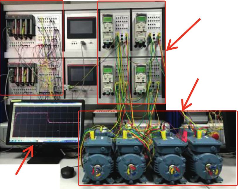
8 Complexity

 Table 3: 4 motor mechanical parameters.
Variable Motor 1 Motor 2 Motor 3 Motor 4
Rated speed (rpm) 1500 1500 1500 1500
Rated torque (N·m) 3 3.3 4.5 4
D-axis self-inductance (mH) 3.5 3.7 4.1 3.8
Q-axis self-inductance (mH) 3.2 3.6 4.0 3.6
Stator resistance (ῼ) 0.9 0.94 1.32 1
Moment of inertia (kg · m2 ) 0.01 0.007 0.005 0.006
Number of pole pairs 2 2 2 2

 Table 4: Sensor fault information.
Sensor Fault type Mathematical description Fault amplitude Time (s)
No. 1, No. 2 Constant deviation (k) � y(k) + c1
 y c1 � − 40, c1′ � − 20 5–6
No. 3, No. 4 Stuck y
 (k) � c2 c2 � 22, c2′ � 18 15–16
No. 2, No. 4 Constant gain y (k) � c3 y(k) c3 � 100, c3′ � 200 25–26

 100 52
 100 51.5
 80 51
 50.5
 Speed (rpm)

 50 50
 Speed (rpm)

 60
 49.5
 25 26 27
 60
 0 40
 40
 20
 0 20
 –50 –20
 15 16 17 18
 0 5 10 15 20 25 30 35
 0
 Time (s) 0 5 10 15 20 25 30 35
 Time (s)
 Subsystem1 Subsystem3
 Subsystem2 Subsystem4 Subsystem1 Subsystem3
 Subsystem2 Subsystem4
Figure 8: Synchronous output without taking any action when two
sensors fail simultaneously. Figure 10: Synchronous output of FTC.

 relatively large (about 2 rad/s) due to the slow change
 34
 32 characteristics of constant gain fault. The synchronization
 error of tolerance is far less than the control error of the
 28
 expected speed change. The fault tolerance is satisfactory
 24 overall.
 Fault indicator

 20 It should be pointed out that, when two sensors have
 different amplitude faults, the distances between the faulty
 16
 sensor and a normal sensor, as well as between two faulty
 12 sensors, become complicated and diverse. It is difficult to
 8 estimate the fault size. In addition, considering the existence
 of the synchronization error and the randomness of the
 4
 distance between different sensors outputs, the threshold
 0 selection is more sensitive.
 0 5 10 15 20 25 30 35
 Time (s)
 5. Experimental Results and Analysis
Figure 9: Fault indication output when two sensors fail
simultaneously. To test the engineering applicability of the proposed method,
 a multimotor synchronous control experimental platform
the remaining two normal sensors are used, and a satis- composed of 4 motors is established. The hardware mainly
factory synchronization performance is achieved. Further- includes ABB’s AC500-eCo PLC; input and output mod-
more, from Figure 11, the synchronization error at t � 25 s is ules DX561, DC562, and AX561; ACS355 frequency

Complexity 9

 2
 Frequency converter
 1.5
 PLC
 Synchronization error (rpm)

 1

 0.5 Motor and encoder

 0

 –0.5

 –1

 –1.5
 Host computer
 –2
 0 5 10 15 20 25 30 35 Figure 12: Semiphysical experiment platform.
 Time (s)
 e1 = y1 – y2 e3 = y3 – y4
 e2 = y2 – y3 e4 = y4 – y1 4

 Figure 11: Synchronization error of FTC. 3.5

 3

 Fault indicator
 2.5
 Table 5: Experimental motor mechanical parameters. 2
Variable Symbol Motor 1.5
Power (kW) P 0.4
Rated voltage (V) U 220 1
Rated current (A) I 1.8 0.5
Rated speed (rpm) N 3000
Rated torque (N·m) T 1.2 0
 0 1 2 3 4 5
Number of pole pairs p 1 Time (s)
 Figure 13: Fault indication output.

converter and permanent magnet synchronous motor (see
Table 5 for parameter information); and 360 line photo-
electric encoder. The software mainly includes Control 2000
Builder Plus (referred to as CBP, integrated with CoDeSys),
OPC configurator, and MATLAB/Simulink. Because the
 1500
AC500-eCo PLC contains only two high-speed counting
 Speed (rpm)

channels, the four motors are controlled by two PLCs
through four frequency converters. The established ex- 1000
perimental platform is shown in Figure 12.
 Setting sensor No. 2–4 to have three kinds of fault,
constant deviation, constant gain, and stuck, the corre- 500
sponding fault occurrence and duration time is 1 − 1.5 s,
2.5 − 3 s, and 4 − 4.5 s, respectively. The expected speed is
2000 rpm. The results of fault diagnosis and fault tolerance 0
 0 1 2 3 4 5
are shown in Figures 13 and 14. Time (s)
 The fault diagnosis is timely and reliable. The design of
 Motor 1 Motor 3
the improved weighted average feedback mechanism based
 Motor 2 Motor 4
on the diagnosis results realized the fault-tolerant control.
The synchronous precision of the system after fault tolerance Figure 14: Synchronous output after fault tolerance.
is satisfactory in the semiphysical experiment. The effec-
tiveness of the method is verified once again in the platform.
It also demonstrates that the fault diagnosis method based 6. Conclusion
on complex network consistent matrix and the tolerance
design of improved weighted mean feedback have good A fault diagnosis and fault-tolerant control method based on
engineering applicability. complex network synchronization has been presented to

10 Complexity

mitigate sensor fault problems in multimotor synchronous [2] M. A. Valenzuela and R. D. Lorenz, “Electronic line-shafting
control. Based on the concept of distance, inspired by the control for paper machine drives,” IEEE Transactions on
idea of the coupling matrix in complex network synchro- Industry Applications, vol. 37, no. 1, pp. 158–164, 2001.
nization, a consistent matrix is devised, which can reflect the [3] D. Xiao, X. Li, and K. He, “Power balance of starting process
similarity of different sensor output data. From the online for pipe belt conveyor based on master-slave control,” IEEE
 Access, vol. 6, pp. 16924–16931, 2018.
correlation of elements and features in the matrix, the sensor
 [4] H.-H. Lian, S.-P. Xiao, Z. Wang, X.-H. Zhang, and H.-Q. Xiao,
fault can be detected, located, and estimated by the element “Further results on sampled-data synchronization control for
value judgments in the matrix. Based on the fault diagnosis chaotic neural networks with actuator saturation,” Neuro-
information, a fault-tolerant mechanism has been designed computing, vol. 346, pp. 30–37, 2019.
by introducing an improved weighted mean feedback to [5] X. Chu, X. Nian, M. Sun, H. Wang, and H. Xiong, “Robust
achieve effective isolation of the faulty sensor. Compared observer design for multi-motor web-winding system,”
with the existing theories and techniques, the proposed Journal of the Franklin Institute, vol. 355, no. 12, pp. 5217–
method has several advantages, such as simple principles, 5239, 2018.
small calculation amount, no need to change the topology [6] R. Shu, J. Wei, D. Qin, T. C. Lim, and A. Zhang, “Global
structure of the original network, easy engineering reali- sensitivity analysis and dynamic optimization of multi-motor
zation, and suitability for single and multiple failure. driving transmission system,” Structural and Multidisciplin-
 From simulations and experiments, in order to imple- ary Optimization, vol. 58, no. 2, pp. 797–816, 2018.
 [7] M. Wang, X. Ren, and Q. Chen, “Robust tracking and dis-
ment satisfactory synchronous control, by considering load
 tributed synchronization control of a multi-motor servo-
interference, noise, and uncertainty, a strong robustness mechanism with H-infinity performance,” ISA Transactions,
control algorithm is necessary when the sensor is normal. In vol. 72, pp. 147–160, 2018.
the meantime, the proposed method can be superimposed [8] K. L. Shi, T. F. Chan, Y. K. Wong, and S. L. Ho, “Speed
on the system as a further synchronous output guarantee. estimation of an induction motor drive using an optimized
The reason is that, due to interference and other factors, extended Kalman filter,” IEEE Transactions on Industrial
when the synchronization error is large at a certain time, the Electronics, vol. 49, no. 1, pp. 124–133, 2002.
method has the function of automatically rejecting the [9] M. Bourogaoui, H. B. A. Sethom, and I. S. Belkhodja, “Speed/
deviation from the larger output, and adopting other closer position sensor fault tolerant control in adjustable speed
output averages as the feedback function, which makes the drives—a review,” ISA Transactions, vol. 64, pp. 269–284,
mean feedback closer to the true value. Therefore, this 2016.
 [10] H. J. Mao, W. Li, K. H. Wang et al., “Sensor fault-tolerant
method can achieve better performance than conventional
 switch strategy study for multi-motor synchronous system
mean feedback, that is, it can realize fault tolerance when
 based on ADRC,” Journal of Shandong University, vol. 47,
there is a fault and improve synchronization accuracy when no. 5, pp. 64–70, 2017.
there is no fault. [11] T. A. Najafabadi, F. R. Salmasi, and P. Jabehdar-Maralani,
 In our future work, the focus will be on the robust and “Detection and isolation of speed-, DC-link voltage-, and
adaptive threshold selection study for multisensor fault current-sensor faults based on an adaptive observer in in-
situation. duction-motor drives,” IEEE Transactions on Industrial
 Electronics, vol. 58, no. 5, pp. 1662–1672, 2011.
 [12] R. Marino, S. Scalzi, P. Tomei, and C. M. Verrelli, “Fault-
Data Availability tolerant cruise control of electric vehicles with induction
The simulation and experimental data used to support the motors,” Control Engineering Practice, vol. 21, no. 6,
 pp. 860–869, 2013.
findings of this study are available from the corresponding
 [13] B. Cai, Y. Zhao, H. Liu, and M. Xie, “A data-driven fault
author upon request. diagnosis methodology in three-phase inverters for pmsm
 drive systems,” IEEE Transactions on Power Electronics,
Conflicts of Interest vol. 32, no. 7, pp. 5590–5600, 2017.
 [14] C. M. Verrelli, S. Bifaretti, E. Carfagna et al., “Speed sensor
The authors declare no conflicts of interest. fault tolerant PMSM machines: from position-sensorless to
 sensorless control,” IEEE Transactions on Industry Applica-
 tions, vol. 55, no. 4, pp. 3946–3954, 2019.
Acknowledgments [15] A. B. Youssef, S. K. El Khil, and I. S. Belkhodja, “Open-circuit
 fault diagnosis and voltage sensor fault-tolerant control of a
This work was supported in part by the National Natural
 single-phase pulsed width modulated rectifier,” Mathematics
Science Foundation of China (Grant nos. 61763027 and and Computers in Simulation, vol. 131, pp. 234–252, 2017.
61873116). [16] X.-J. Li and G.-H. Yang, “Adaptive fault-tolerant synchro-
 nization control of a class of complex dynamical networks
References with general input distribution matrices and actuator faults,”
 IEEE Transactions on Neural Networks and Learning Systems,
 [1] I. X. Bogiatzidis, A. N. Safacas, E. D. Mitronikas, and vol. 28, no. 3, pp. 559–569, 2017.
 G. A. Christopoulos, “A novel control strategy applicable for a [17] C. Chen, X. Zhou, Z. Li, Z. He, Z. Li, and X. Lin, “Novel
 dual AC drive with common mechanical load,” IEEE complex network model and its application in identifying
 Transactions on Industry Applications, vol. 48, no. 6, critical components of power grid,” Physica A: Statistical
 pp. 2022–2036, 2012. Mechanics and Its Applications, vol. 512, pp. 316–329, 2018.

Complexity 11

[18] L. Ding, Q.-L. Han, and X.-M. Zhang, “Distributed secondary
 control for active power sharing and frequency regulation in
 islanded microgrids using an event-triggered communication
 mechanism,” IEEE Transactions on Industrial Informatics,
 vol. 15, no. 7, pp. 3910–3922, 2019.
[19] C. Zhang, J. Wang, D. Zhang, and X. Shao, “Fault-tolerant
 adaptive finite-time attitude synchronization and tracking
 control for multi-spacecraft formation,” Aerospace Science
 and Technology, vol. 73, pp. 197–209, 2018.
[20] M. Tomizuka, J. Hu, and K. T. Chiu, “Synchronization of two
 motion control axes under adaptive feed-forward control,”
 ASME Journal of Dynamic Systems. Measurement and Con-
 trol, vol. 114, pp. 3234–3245, 1992.
[21] F. Perez-Pinal, G. Caladeron, R. Alvarez et al., “Comparison of
 multi-motor synchronization techniques,” in Proceedings of
 the 30th Annual Conference of the IEEE Industrial Electronics
 Society, pp. 1670–1675, Busan, Korea, November 2004.
[22] T. Shi, H. Liu, Q. Geng, and C. Xia, “Improved relative
 coupling control structure for multi-motor speed synchro-
 nous driving system,” IET Electric Power Applications, vol. 10,
 no. 6, pp. 451–457, 2016.
[23] F.-J. Lin, P.-H. Chou, C.-S. Chen, and Y.-S. Lin, “DSP-based
 cross-coupled synchronous control for dual linear motors via
 intelligent complementary sliding mode control,” IEEE
 Transactions on Industrial Electronics, vol. 59, no. 2,
 pp. 1061–1073, 2012.
[24] W. Limei and H. Fei, “Research on synchro drive technique of
 dual motor based on decoupling control and internal model
 control,” in Proceedings of the 2009 Chinese Control and
 Decision Conference (CCDC), pp. 5334–5337, Guilin, China,
 June 2009.
[25] L. Zhou, J. She, X. Zhang et al., “Performance enhancement of
 repetitive-control systems and application to tracking control
 of chuck-workpiece systems,” IEEE Transactions on Industrial
 Electronics, vol. 67, no. 5, pp. 4056–4065.
[26] L. Zhou, J. She, S. Zhou, and C. Li, “Compensation for state-
 dependent nonlinearity in a modified repetitive control sys-
 tem,” International Journal of Robust and Nonlinear Control,
 vol. 28, no. 1, pp. 213–226, 2018.
[27] B.-L. Zhang, Q.-L. Han, X. Zhang et al., “Sliding mode control
 with mixed current and delayed states for offshore steel jacket
 platforms,” IEEE Transactions on Control Systems Technology,
 vol. 22, no. 5, pp. 1769–1783, 2014.
[28] J. Chen, J. A. Lu, and J. Zhou, “On the relationship between
 the synchronous state and the solution of an isolated node in a
 complex network,” Acta Automatic Sinica, vol. 39, no. 12,
 pp. 2111–2120, 2013.
[29] L. Guo and X. M. Xu, Complex Network, Shanghai Science and
 Technology Education Publishing House, Shanghai, China,
 2006.