Gas Classification Using Deep Convolutional Neural Networks - MDPI
←
→
Page content transcription
If your browser does not render page correctly, please read the page content below
sensors
Article
Gas Classification Using Deep Convolutional
Neural Networks
Pai Peng 1,3 , Xiaojin Zhao 1 , Xiaofang Pan 2 and Wenbin Ye 1, *
 1   School of Electronic Science and Technology, Shenzhen University, Shenzhen 518060, China;
     pengpai_sh@szu.edu.cn (P.P.); eexjzhao@szu.edu.cn (X.Z.)
 2   School of Information Engineering, Shenzhen University, Shenzhen 518060, China; eexpan@szu.edu.cn
 3   Key Laboratory of Optoelectronic Devices and Systems of Ministry of Education and Guangdong Province,
     College of Optoelectronic Engineering, Shenzhen University, Shenzhen 518060, China
 *   Correspondence: yewenbin@szu.edu.cn; Tel.: +86-755-2672-3212

 Received: 8 November 2017; Accepted: 30 December 2017; Published: 8 January 2018

 Abstract: In this work, we propose a novel Deep Convolutional Neural Network (DCNN) tailored for
 gas classification. Inspired by the great success of DCNN in the field of computer vision, we designed
 a DCNN with up to 38 layers. In general, the proposed gas neural network, named GasNet, consists of:
 six convolutional blocks, each block consist of six layers; a pooling layer; and a fully-connected layer.
 Together, these various layers make up a powerful deep model for gas classification. Experimental
 results show that the proposed DCNN method is an effective technique for classifying electronic nose
 data. We also demonstrate that the DCNN method can provide higher classification accuracy than
 comparable Support Vector Machine (SVM) methods and Multiple Layer Perceptron (MLP).

 Keywords: gas classification; deep convolutional neural networks; electronic nose

1. Introduction
     The electronic nose, which imitates the perceptual mechanisms found in biological olfactory
organs, has been widely used in many applications for a variety of purposes including medicine and
diagnostics [1], food production [2] and environment monitoring [3,4]. A conventional electronic nose
typically consists of three parts: a gas sensor array that is a set of chemical sensors which convert the
chemical smell signal to an electronic signal; a preprocessing block that extracts the features of the
gas signal; and a pattern recognition system that can recognize the olfactory features of the substance
being tested. In this paper, we focus upon just the third part.
     In the past several decades, many pattern recognition algorithms have been proposed for gas
classification. With regard to electronic nose applications, the K-Nearest Neighbor (KNN) method
was introduced in [5,6]. This method is quite simple and effective, but involves the storing of
training data. As a result, this is not a suitable approach when memory is limited. In order to
overcome this shortcoming, a Gaussian Mixture Model (GMM) approach was proposed for odor
classification in [7]. In this case, transient features are used that offer the possibility of real-time
classification. In [8–10], a multiple layer perception (MLP) network is used to address the nonlinearity
present in odor classification. However, in this case, the need for a full connection can cause the
classifier to get trapped in overfitting, leading to a bad prediction. A Support Vector Machine (SVM),
by contrast, is an advanced supervised classification technique that outperforms Artificial Neural
Network (ANN) models, particularly when only a small data-set is available for training [11,12]. In [13],
a recently developed machine learning technique, the Relevance Vector machine (RVM), is proposed
instead. An RVM is similar to an SVM but requires fewer kernel functions. In [14], deep Restricted
Boltzmann Machines (RBM) are proposed as a way of using electronic noses to identify bacteria in
blood. Similarly, Liu et al. [15] suggest that gas recognition under drift might be accomplished by

Sensors 2018, 18, 157; doi:10.3390/s18010157                                 www.mdpi.com/journal/sensors
Sensors 2018, 18, 157 2 of 11
using a deep Boltzmann Machine and a Sparse Auto-Encoder (SAE). However, these two models are
rather, when compared to the Deep Convolutional Neural Networks (DCNNs), used in computer
vision. With RBM and SAE, the depth is usually 3–4 layers, with 1–2 of them being hidden, as opposed
to the dozens to hundreds layers offered by DCNNs. Moreover, RBM and SAE are unsupervised
learning techniques. In other words, they try to learn a hidden representation pattern, with the learned
features then being fed into another classification framework, making feature extraction/learning and
classification quite distinct.
In this paper, an end-to-end (DCNN) called GasNet that is tailored for gas classification is
proposed. The motivation of adopting DCNN is that the DCNN has the ability to jointly learn
the features and classification boundaries directly from raw input data. In the DCNN architecture,
the convolutional kernels work as filters that can automatically extract the features of the raw input
data. The performance of classical approaches such as SVM and MLP is very related to the prior
knowledge and human effort in feature extraction. However, for a certain gas dataset, to find a good
feature extraction method is already a difficult task and needs much prior knowledge of that dataset.
The proposed GasNet consists of: six convolutional blocks; a pooling layer; and a fully-connected
layer. Each convolutional block that consists of six layers, i.e., two convolutional layers, two batch
normalization layers and two Rectified linear unit (ReLU) layers are proposed to extract highly
representative features and thus the proposed DCNN is up 38 layers. Together, these various layers
make up a powerful deep model for gas classification. Compared with previously proposed methods,
this DCNN has two particularly significant advantages. Firstly, because SVM, KNN, and GMM are
all typical conventional machine learning algorithms, a DCNN is better at mining and extracting
effective features. This is thanks to the large amount of nonlinear activation neurons in the network
architecture. Secondly, a DCNN is an end-to-end deep network, while RBM and SAE break the whole
framework into two independent parts, i.e., feature learning and gas classification. An end-to-end
approach offers better performance because there is less information loss. The contribution of this
paper can be summarized as follows:
(1) We propose a very deep convolutional neural network called GasNet for gas classification. To the
best of our knowledge, our work is the first one to exploit a real “deep” learning-based model to
recognize gas types.
(2) The proposed CNN contains up to 38 layers. This offers huge advantages over conventional
machine learning algorithms (e.g., SVM, KNN, and GMM) and other recently proposed more
shallow networks (e.g., RBM and SAE).
(3) Experimental results confirm that GasNet achieves higher classification accuracy than other
previous approaches.
The rest of this article is organized as follows. In the next section, the proposed GasNet is presented.
Section 3 discusses the experimental results that compare the performance of the classification accuracy
of different classifier methods. Some concluding remarks are given in Section 4.
2. The Proposed GasNet Tailored for the Gas Classification
In this section, we describe the proposed GasNet DCNN in more detail. First of all, we provide
an overview of GasNet and how it is suitable for gas classification. We then elaborate upon each
component/layer in the network architecture. After this, we present the network training schedule.
2.1. GasNet Overview
Deep learning is the process of training a (deep) neural network given a specific task. A neural
network is nothing but a large and complex mathematical function with millions of parameters.
Thus, deep learning has great power to learn the decision function by feeding in input and expected
output (we call training data). Creating or “training” this function functionality requires a large
amount of training data because of the huge number of parameters. At the beginning of the trainingSensors 2018, 18, 157 3 of 11
process, the parameters are set to random values (or values generated with a normal distribution).
Then, for each data example in the training set, the loss (or error) value is computed as the difference
between the expected output (what we call ground truth) and predictions. After that, the values of
the parameters are slightly changed so as to decrease the loss by using an effective schedule called a
Stochastic Gradient Descent (SGD). This process is repeated for every data example in the training set
many times over. As a result, the neural network is able to learn decision functions, assuming enough
training data is provided.
In recent years, we have witnessed a revolutionary trend in the field of computer vision. DCNNs
have become the state-of-the-art for visual recognition and understanding. The key to the success of
DCNNs is the convolutional operation or convolutional layer, which can automatically learn useful
implicit features according to the intensity of pixels in input images. The key to the success of DCNN
is the convolutional operation or convolutional layer that is able to automatically learn useful implicit
features from the intensities of the pixels in the input images. The ImageNet challenge [16] has been
especially notable in how it has contributed to the birth of a variety of effective DCNN architectures
such as AlexNet [17] (ImageNet 2012 winner), Zeiler-Fergus (ZF)-Net [18] (ImageNet 2013 winner),
Visual Geometry Group(VGG)-Net [19] (ImageNet 2014 winner), ResNet [20] (ImageNet 2015 winner)
and Inception series [21,22]. However, they cannot be applied to gas classification directly because,
first of all, existing DCNNs are specifically designed for processing visual data. As a result, the input
is usually a high-dimensional image with three channels (in the RGB color space), e.g., 299 × 299 × 3.
The dimensionality of features collected by gas sensors, however, is quite a bit lower, e.g., each sensor
generates a 16D feature vector. Another issue is that the cost of obtaining large scale visual data is
much lower than it is for gas data. Finally, the pre-trained weights (parameters) of DCNNs for visual
data are publicly available while there are no pre-trained weights available for gas data (Our work is
the first one to exploit DCNNs to recognize gas types). Because of these issues, in order to leverage
deep learning for recognizing gas types, we have had to carefully design a novel DCNN that can
accept gas feature vectors as input and then output a gas class label. The nuts and bolts of the deep
network architecture are covered in the next section.
2.2. Network Architecture
Overall, GasNet is composed of convolutional, batch normalization pooling operations. For the
sake of feature representational power, a few convolutional and batch normalization operations
together make up a computational unit that we call “convolutional block”. In the rest of this section,
we describe the overall network architecture and then detail the convolutional block components.
2.2.1. Overall Architecture
Figure 1 depicts the proposed overall network architecture. It begins with an input layer,
which accepts a feature tensor with the shape of m × n, where m is the number of sensors and n
is the dimensionality for each sensor. Then, a stack of convolutional blocks are applied in order to extract
useful and highly representative features. Motivated by the design philosophy of VGG-Net [19] and
ResNet [20], the network follows two design rules: (1) the number of feature maps keeps the same
when the layer’s output shape is preserved; (2) the number of feature maps doubles when the layer’s
output shape is reduced by a half. These two design concepts ensure that the computational cost is
roughly the same for each convolutional block. Overall, GasNet includes three max-pooling layers
and each reduces the output resolution by a half. A global average pooling layer is followed by the
last convolutional block. A global average pooling operation is usually used to distill the crucial
information while removing redundancy. Finally, GasNet ends with a fully connected layer with
number of types of neurons and Softmax activation. Note that, inspired by [20], we add shortcut
(or skipped connection) for convolutional blocks. This helps to avoid any “gradient vanishing”
problem. In other words, the gradients will flow back through the shortcut during back-propagation,
so that the gradients can skip over the adjacent convolutional block to reach the next one.Sensors 2018, 18, 157 4 of 11
Input m×n×1
Convolutional Block (32) m×n×32
shortcut
Convolutional Block (32) m×n×32
shortcut Pool / 2
Convolutional Block (64) (m/2)×(n/2)×64
shortcut
Convolutional Block (64) (m/2)×(n/2)×64
shortcut Pool / 2
Convolutional Block (128) (m/4)×(n/4)×128
shortcut
Convolutional Block (128) (m/4)×(n/4)×128
Global Average Pooling 1×1×128
Fully connected ,Nbr_classes 1×1×C
Figure 1. GasNet architecture.
In summary, the input tensor shape for GasNet is m × n × 1, followed by six convolutional blocks
separated by two max-pooling operations. The output tensor shape becomes m4 × n4 × 128 right after
the last convolutional block. Next, the global average pooling layer averages the activations for each
feature map and outputs a tensor with shape of 1 × 1 × 128. Lastly, the GasNet outputs C values for
each input vector and each represents the probability of being that specific gas type.
2.2.2. Convolutional Block
As shown in Figure 2, each convolutional block consists of two typical convolutional layers
and each one is followed by a batch normalization (BN) [23] layer and ReLU activation function.
The convolutional operation is illustrated as Figure 3. Convolution is the process of adding each
element of the 2D matrix to its local neighbors, weighted by the kernel as shown in Figure 3. Assume
that input matrix A has dimensions (Ma, Na) and kernel matrix B has dimensions (M, N). When the
block calculates the full output size, the equation for the 2D discrete convolution can be expressed as
Ma−1 Na−1
C (i, j) = ∑ ∑ A(m, n) × B(i − m, j − n), (1)
m =0 n =0
where 0 ≤ i < Ma + M − 1 and 0 ≤ j < Na + N − 1. BN is a useful recently proposed technique that
can potentially help in two ways, by providing: faster learning and higher overall accuracy. Frequently,
normalization (i.e., shifting inputs to zero mean and unit variance) is used as a pre-processing step
to make data comparable across features. As the data flows through a deep network, the weights
and parameters adjust these values, sometimes making the data too big or too small again. This is a
problem that is referred to as “internal covariate shift”. BN is used to normalize the data in a mini-batch
during the network training process. The convolutional kernel size is fixed to 3 × 3 and padding is
1 so that the output shape is the same as the input within one block.Sensors 2018, 18, 157 5 of 11
Convolution, 3×3, 32
Batch Normalization
ReLU
Convolution, 3×3, 32
Batch Normalization
ReLU
Figure 2. Convolutional block.
Kernel
Input Output
Figure 3. Convolution operation illustration.
In our view, the convolutional block we have designed has two advantages: (1) it introduces more
nonlinearity into the network by stacking two consecutive convolutional layers; (2) the number of
parameters is limited due to having 3 × 3 kernels, so stacking more convolutional blocks to increase the
depth of the network is feasible. Suppose the input kernel size is 3 × 3 and the number of input channels
and output channels are both c. Then, a single output feature map contains 3 × 3 × c parameters.
Note that we have c feature maps. Thus, the total number of parameters is 3 × 3 × c × c, which is 9c2 .
Thus, one single convolutional block contains 18c2 (parameters for BN could be omitted).
2.3. Network Training
Loss Function Cross-entropy is frequently used for loss/error calculations in classification tasks
in deep learning. Ideally, the error should be 0 if the deep network (the classifier) is perfectly classifying
an unseen data sample during the testing stage. Failing this, some error (between 0 and 1) is computed
as a punishment on the classifier. As the network encounters more and more data, it tends to predict
more and more precisely. If we let y be the ground truth label for a certain data point x and ŷ is the
prediction generated by the classifier. The cross-entropy error for this specific data point is defined
as follows:
C
L(y, y)ˆ = − ∑ yi log ŷi , (2)
i =1
where C is the number of classes in the dataset. It is worth noting that the overall loss is the averaged
loss over all the training data.Sensors 2018, 18, 157 6 of 11
Optimization For our DCNN, we use Stochastic Gradient Descent (SGD) as the optimization
method. The initial learning rate is set at 0.01 and the momentum at 0.9. We decrease the learning
rate by a factor of 0.1 if the accuracy stops increasing for five epochs until it reaches 0.00001. In order
to prevent from overfitting, we also use an early stop strategy. All network weights were initialized
following the suggestions proposed in [24], i.e., variance of neurons in the network should be 2/n (n is
the number of neurons in the layer).
3. Experimental Results
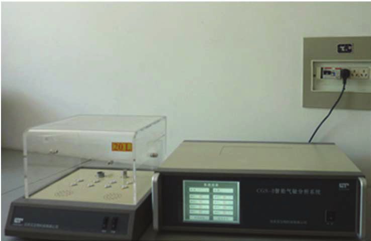
The automated gas delivery setup used to acquire response data of target gases with the sensor
array is shown in Figure 4. Eight commercial Figaro metal oxide semiconductor (MOS) sensors
(Arlington Heights , IL, USA) are used to build the gas sensor array and their corresponding part
numbers are listed in Table 1. The electronic signals of these sensors are simultaneously acquired
through a chemical gas sensor CGS-8 system in 10 Hz sampling rate. The flow rate of the target gas
can be controlled by the computer controlled mass flow controllers (MFCs) . Through changing the
ratio of the flow rate between target gas and background gas, we can get a range of concentrations
of target gas. In our experiment, there are 20 concentrations for each gas. For each type of gas
at each concentration, we make 15 repeated measurements and thus there are 300 measurements
for each type of gas. As there are four types of gases (Carbon Monoxide, Methane, Hydrogen and
Ethylene) in our case, we totally have 300 × 4 = 1200 samples in our data sets. In our experiment,
the measurement for each gas at certain concentration last 100 s. Therefore, for each measurement,
there are 100 × 10 = 1000 points for each sensor. The gas sensor array consists of eight sensors and
thus there are there are 100 × 10 × 8 = 8000 points in each raw sample data. Without any additional
feature engineering, the raw sampled data is directed taken as the input of the SVM, MLP and the
proposed DCNN method. We randomly split the dataset into 70% training and 30% test sets. In other
words, for each type of gas, 300 × 0.7 = 210 samples (each sample is 8000 × 1 column vector) are
selected for training the classifiers, while the rest samples are used to test the classifiers. Therefore,
the overall training samples is 210 × 4 = 840 Since the training set and test set are randomly selected
from the whole dataset, to eliminate the bias of the test result, we then repeated this train-test procedure
100 times with different random splits. Then, we average the accuracy of each test to get the accuracy
for each classifier.
PC
Air MFC
DAQ
Gas 1 MFC
Sensor
Array
Gas 2 MFC Gas Chamber
Gas n MFC
Figure 4. Experimental setup to acquire signatures of the target gases with the sensor array.Sensors 2018, 18, 157 7 of 11
Table 1. Types of metal oxide semiconductor (MOS) sensors (provided by Figaro Inc. (Arlington
Heights, IL, USA)).
Channel Sensor Part Number
0 TGS821
1 TGS812
2 TGS2610
3 TGS2612
4 TGS3870
5 TGS2611
6 TGS816
7 TGS2602
3.1. Baseline Approach
SVM—Before the widespread adoption of neural networks in recent years, support vector
machines (SVM) [12] were the dominant pattern recognition and classification tool. A great deal
of research effort was devoted to exploiting SVMs for gas classification. For this reason, SVM was
chosen as one of our baseline approaches. It should be noted that an L-SVM is proposed in [25] .
The L-SVM is an ensemble method and can achieve higher classification accuracy than single SVM
if there is some drift between the training data and test data, since there is no drift in our dataset
and thus the L-SVM method is not compared in our paper. Since the input for an SVM is usually a
one-dimensional feature vector, we stretched the input tensor for GasNet by rows. In other words,
we reshaped a three-dimensional tensor m × n × 1 to a one-dimensional vector m ∗ n. We trained SVM
with an Radial basis function (RBF) kernel. The kernel bandwidth parameter γ and punish function
C parameter were chosen using a 5-fold cross validation by performing a grid search in the range
−7 −6
2 , 2 , . . . , 26 , 27 and 2−7 , 2−6 , . . . , 28 , 29 , respectively. In the proposed 5-fold cross-validation,
the original sample is randomly partitioned into five equal sized subsamples. A single subsample is
retained as the validation data for testing the model, and the remaining four subsamples are used as
training data. The cross-validation process is then repeated five times. Then, the five results from the
folds are averaged to produce a single estimation.
MLP—New research [10] has proposed a real-time gas classification service system that uses a
Multi-Layer Perceptron (MLP) artificial neural network to detect and classify gas sensor data. MLP is
actually a simple neural network with a hidden layer (excluding the input layer and output layer).
In the MLP, the number of hidden layers is 1 and the neurons in each hidden layer is 1024.
3.2. Learning Curves
Learning curves are one of the most important evaluation measures for machine/deep learning
algorithms. As can be seen in Figure 5, training accuracy and validation accuracy maintain a steady
increase as the number of training iterations increases. Similarly, in Figure 6, it can be seen that training
loss and validation loss continue to decrease as the number of epochs goes up. Based on the learning
curves, we can conclude that we didn’t incur an “overfitting” or “underfitting” phenomenon.Sensors 2018, 18, 157 8 of 11
GasNet Accuracy
1
0.9
0.8
0.7
0.6 Train
Accuracy
0.5 Val
0.4
0.3
0.2
0.1
0
0 20 40 60 80 100
Epoch
Figure 5. Accuracy.
GasNet Loss
1.5
Train
Val
1
Loss
0.5
0
0 20 40 60 80 100
Epoch
Figure 6. Loss.
3.3. Performance of Recognition
Classification/recognition accuracy is one of the most important evaluation metrics for supervised
learning algorithms. For this, the number of correctly recognized examples is divided by the total
number of testing examples. Recognition accuracy performance is summarized in Table 2. SVM is a
typical example of the “shallow learning” school. Thus, it is no wonder that SVM achieves similar
performance results to MLP. It can be seen that our proposed GasNet outperforms SVM and MLP by
some margin. There are three reasons for this: (1) GasNet is a much deeper neural network compared
with SVM or MLP; (2) the convolutional block contains more than one convolutional layer, making
GasNet more representative; and (3) the kernel size is tailored for a gas classification scenario, helping
the network to learn more expressive and discriminative features.Sensors 2018, 18, 157 9 of 11
Table 2. Performance of recognition accuracy.
Model Validation Accuracy Training Time(s)
SVM 79.9% 2
MLP 82.3% 17
GasNet 95.2% 154
3.4. The Computational Complexity of the DCNN
The computational cost of the machine learning methods can be divided into two parts that is
training and estimation. The training time for the different methods is listed in Table 1. And it can
be seen that the proposed CNN has the highest computational time in the training part. However,
the training computational complexity is not very important, as the training operation is performed
offline and in most cases is performed just once. Therefore, in our cases, only the operational
computational cost of MLP, SVM and the proposed CNN is compared. The operational computational
cost of SVM is O(ns vd), where ns v is the number of support vectors, d is the input data dimension
that can be expressed as m × n, m is the number of gas sensors and n is the dimensionality for
each sensor. For the MLP, the computational complexity can be expressed as O(nl kd), where
nl is the number of hidden layers, and k is the number of neurons in each layer. As for the
proposed CNN, the convolutional operation dominates the overall computational complexity and
thus, for the computational complexity estimation, only convolutional operation are taken into account.
There are two convolution layers in the proposed convolution block. For each convolution layer,
the computational cost is 2 × m × n × M × N × L, where, M × N is the size of the convolutional
kernel and L is the number of kernels. Since there are six convolution blocks, the overall computational
cost of the proposed CNN can be estimated as O(12d × M × N × L). In our case, the kernel size is
3 × 3, and the kernel number L is 32. Generally, the operational computational cost of the proposed
CNN is much higher than SVM and MLP. In other words, DCNN achieves the higher classification
accuracy at the cost of higher computational complexity than MLP and SVM.
4. Conclusions
In this work, we have presented a method for leveraging deep learning for the recognition of
gas types. To do this, we designed a novel DCNN that can accept gas feature vectors as input and
then output a gas class label. As far as we know, this is the first DCNN that has been used for gas
classification. DCNNs are better at mining and extracting effective features because of the large number
of nonlinear activation neurons in the network architecture, resulting in higher classification accuracy
than that of conventional methods such as SVM or MLP. Our experimental results have served to
verify this claim.
Acknowledgments: This work was supported by the National Natural Science Foundation of China (Grant
No. 61504087), the Fundamental Research Foundation of Shenzhen (Grant No. JCYJ20160308094919279,
JCYJ20170302151123005), the Key Project Department of Education of Guangdong Province (No. 2015KQNCX142)
and the Natural Science Foundation of Shenzhen University (Grant No. 2016020).
Author Contributions: The work presented in this paper is a collaborative development by all of the authors.
Wenbin Ye and Pai Peng contributed to the idea of the incentive mechanism and designed the algorithms.
Xiaojin Zhao and Xiaofang Pan were responsible for some parts of the theoretical analysis and the paper check.
All of the authors were involved in writing the paper.
Conflicts of Interest: The authors declare no conflict of interest.
References
1. Kiani, S.; Minaei, S.; Ghasemi-Varnamkhasti, M. Application of electronic nose systems for assessing quality
of medicinal and aromatic plant products: A review. J. Appl. Res. Med. Aromat. Plants 2016, 3, 1–9. [CrossRef]Sensors 2018, 18, 157 10 of 11
2. Loutfi, A.; Coradeschi, S.; Mani, G.K.; Shankar, P.; Rayappan, J.B.B. Electronic noses for food quality: A review.
J. Food Eng. 2015, 144, 103–111. [CrossRef]
3. Romain, A.C.; Nicolas, J. Long term stability of metal oxide-based gas sensors for e-nose environmental
applications: An overview. Sens. Actuators B Chem. 2010, 146, 502–506. [CrossRef]
4. Capelli, L.; Sironi, S.; Del Rosso, R. Electronic noses for environmental monitoring applications. Sensors 2014,
14, 19979–20007. [CrossRef] [PubMed]
5. Gutierrez-Osuna, R.; Gutierrez-Galvez, A.; Powar, N. Transient response analysis for temperature-modulated
chemoresistors. Sens. Actuators B Chem. 2003, 93, 57–66. [CrossRef]
6. Yang, J.; Sun, Z.; Chen, Y. Fault detection using the clustering-kNN rule for gas sensor arrays. Sensors 2016,
28, 2069. [CrossRef] [PubMed]
7. Belhouari, S.B.; Bermak, A.; Shi, M.; Chan, P.C. Fast and robust gas identification system using an integrated
gas sensor technology and Gaussian mixture models. IEEE Sens. J. 2005, 5, 1433–1444. [CrossRef]
8. Brezmes, J.; Ferreras, B.; Llobet, E.; Vilanova, X.; Correig, X. Neural network based electronic nose for the
classification of aromatic species. Anal. Chim. Acta 1997, 348, 503–509. [CrossRef]
9. Omatul, S.; Yano, M. Mixed Odors Classification by Neural Networks. In Proceedings of the 2015 IEEE 8th
International Conference on Intelligent Data Acquisition and Advanced Computing Systems: Technology
and Applications (IDAACS), Warsaw, Poland, 24–26 September 2015; pp. 171–176.
10. Zhai, X.; Ali, A.A.S.; Amira, A.; Bensaali, F. MLP neural network based gas classification system on Zynq
SoC. IEEE Access 2016, 4, 8138–8146. [CrossRef]
11. Acevedo, F.; Maldonado, S.; Dominguez, E.; Narvaez, A.; Lopez, F. Probabilistic support vector machines for
multi-class alcohol identification. Sens. Actuators B Chem. 2007, 122, 227–235. [CrossRef]
12. Lentka, Ł.; Smulko, J.M.; Ionescu, R.; Granqvist, C.G.; Kish, L.B. Determination of gas mixture components
using fluctuation enhanced sensing and the LS-SVM regression algorithm. Metrol. Meas. Syst. 2015, 3,
341–350.
13. Wang, X.; Ye, M.; Duanmua, C. Classification of data from electronic nose using relevance vector machines.
Sens. Actuators B Chem. 2009, 140, 143–148. [CrossRef]
14. Langkvist, M.; Loutfi, A. Unsupervised feature learning for electronic nose data applied to Bacteria
Identification in Blood. In Proceedings of the NIPS 2011 Workshop on Deep Learning and Unsupervised
Feature Learning, Granada, Spain, 12–17 December 2011; pp. 1–7.
15. Liu, Q.; Hu, X.; Ye, M.; Cheng, X.; Li, F. Gas recognition under sensor drift by using deep learning. Int. J.
Intell. Syst. 2015, 30, 907–922. [CrossRef]
16. Available online: http://www.image-net.org/ (accessed on 13 September 2017).
17. Krizhevsky, A.; Ilya, S.; Hinton, G.E. ImageNet classification with deep convolutional neural networks. NIPS
2012, 1, 1097–1105. [CrossRef]
18. Zeiler, D.; Fergus, R. Visualizing and understanding convolutional networks, in: Computer Vision.
In Proceedings of the 13th European Conference in Computer Vision, Zurich, Switzerland, 6–12 September
2014; pp. 818–833.
19. Simonyan, K.; Zisserman, A. Very deep convolutional networks for large-scale image recognition. arXiv
2014, arXiv:1409.1556v6.
20. He, K.; Zhang, X.; Ren, S.; Sun, J. Deep residual learning for image recognition. In Proceedings of the 2016
IEEE Conference on Computer Vision and Pattern Recognition (CVPR), Las Vegas, NV, USA, 27–30 June
2016; pp. 770–778.
21. Szegedy, C.; Ioffe, S.; Vanhoucke, V.; Alemi, A. Rethinking the inception architecture for computer vision.
In Proceedings of the 2016 IEEE Conference on Computer Vision and Pattern Recognition (CVPR), Las Vegas,
NV, USA, 27–30 June 2016; pp. 2818–2826.
22. Szegedy, C.; Ioffe, S.; Vanhoucke, V.; Alemi, A. Inception-v4, inception-resnet and the impact of residual
connections on learning. In Proceedings of the Thirty-First AAAI Conference on Artificial Intelligence,
San Francisco, CA, USA, 4–9 February 2017; pp. 4278–4284.
23. Ioffe, S.; Szegedy, C. Batch normalization: Accelerating deep network training by reducing internal covariate
shift. In Proceedings of the 32nd International Conference on Machine Learning, ICML, Lille, France,
6–11 July 2015; pp. 448–456.Sensors 2018, 18, 157 11 of 11
24. He, K.; Zhang, X.; Ren, S.; Sun, J. Surpassing human-level performance on imagenet classification.
In Proceedings of the IEEE International Conference on Computer Vision, Santiago, Chile, 7–13 December
2015; pp. 1026–1034.
25. Vergara, A.; Vembu, S.; Ayhan, T.; Ryan, M.; Homer, M.L.; Huerta, R. Chemical gas sensor drift compensation
using classifier ensembles. Sens. Actuators B Chem. 2012, 9, 320–329. [CrossRef]
© 2018 by the authors. Licensee MDPI, Basel, Switzerland. This article is an open access
article distributed under the terms and conditions of the Creative Commons Attribution
(CC BY) license (http://creativecommons.org/licenses/by/4.0/).You can also read


