ASSESSMENT OF DESIGN AND ANALYSIS FRAMEWORKS FOR ON-FARM EXPERIMENTATION THROUGH A SIMULATION STUDY OF WHEAT YIELD IN JAPAN - arXiv.org
←
→
Page content transcription
If your browser does not render page correctly, please read the page content below
A SSESSMENT OF DESIGN AND ANALYSIS FRAMEWORKS FOR
                                               ON - FARM EXPERIMENTATION THROUGH A SIMULATION STUDY
                                                               OF WHEAT YIELD IN JAPAN

                                                                                            Takashi S. T. Tanaka
arXiv:2004.12741v2 [stat.AP] 15 Mar 2021

                                                                                   Faculty of Applied Biological Sciences
                                                                                               Gifu University
                                                                                    1-1 Yanagido, Gifu, Japan 5011193
                                                                                        takashit@gifu-u.ac.jp

                                                                                                March 16, 2021

                                                                                                A BSTRACT
                                                    On-farm experiments can provide farmers with information on more efficient crop management in
                                                    their own fields. Developments in precision agricultural technologies, such as yield monitoring and
                                                    variable-rate application technology, allow farmers to implement on-farm experiments. Research
                                                    frameworks including the experimental design and the statistical analysis method strongly influences
                                                    the precision of the experiment. Conventional statistical approaches (e.g., ordinary least squares
                                                    regression) may not be appropriate for on-farm experiments because they are not capable of accurately
                                                    accounting for the underlying spatial variation in a particular response variable (e.g., yield data). The
                                                    effects of experimental designs and statistical approaches on type I error rates and estimation accuracy
                                                    were explored through a simulation study hypothetically conducted on experiments in three wheat
                                                    fields in Japan. Isotropic and anisotropic spatial linear mixed models were established for comparison
                                                    with ordinary least squares regression models. The repeated designs were not sufficient to reduce
                                                    both the risk of a type I error and the estimation bias on their own. A combination of a repeated
                                                    design and an anisotropic model is sometimes required to improve the precision of the experiments.
                                                    Model selection should be performed to determine whether the anisotropic model is required for
                                                    analysis of any specific field. The anisotropic model had larger standard errors than the other models,
                                                    especially when the estimates had large biases. This finding highlights an advantage of anisotropic
                                                    models since they enable experimenters to cautiously consider the reliability of the estimates when
                                                    they have a large bias.

                                           Keywords Anisotropic variograms · experimental design · linear mixed models · remote sensing · sum-metric model

                                           1    Introduction
                                           On-farm experimentation is a means of farmer-centric research and extension that examines the effect of crop man-
                                           agement (e.g., fertilizer application, irrigation, and pest control) and variety selection on crop productivity in farmers’
                                           own fields [1, 2]. Since the last century, agricultural experiments have been primarily performed by researchers in
                                           experimental fields under highly controlled conditions to ensure the accuracy of the estimated treatment effects. This
                                           typical research approach has contributed to an improved understanding of crop physiology and to developing agronomic
                                           practices, but the research results are not straightforwardly tailored to entire fields or regions. Thus, farmers and crop
                                           advisors have learned how to adjust crop management techniques by trial and error on farms [3]. Developments in
                                           precision agricultural technologies, such as yield monitoring for combine harvesters and variable-rate application (VRA)
                                           technology (e.g., fertilizers, seeds and herbicides), allow farmers to run experiments on their own farms (Hicks et al.
                                           [4, 5, 6]. On-farm experimentation has been gaining popularity by providing information on the best crop management
                                           techniques for specific regions, farmers, and fields [2]. This increased popularity has identified new challenges for the
                                           implementation of on-farm experiments.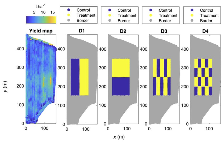
A PREPRINT - M ARCH 16, 2021

      To evaluate the precise effect of genotype and crop management on crop productivity, conventional small-plot
experiments have been widely applied in agricultural research. These conventional small-plot experiments depend on
the combination of three basic principles of experimental design (randomization, replication, and local control) and
statistical approaches, such as analysis of variance (ANOVA), which were established by Fisher [7]. This fundamental
agronomic research framework effectively separates the spatial variations and measurement errors from the observed
data to detect the significance of the treatment effect [1]. Widely used conventional statistical approaches, including
ANOVA and ordinary least squares (OLS) regression, depend on the assumption that errors are independent. However,
soil properties and crop yield are not spatially distributed at random, and similar values are observed near each other,
which is called spatial autocorrelation [8]. Spatial autocorrelation in a response variable (e.g., the crop yield) violates a
conventional statistical assumption of independent errors, which leads to unreliable inferences (e.g., overestimation
of the treatment effects) [9, 10]. Thus, conventional statistical approaches are not directly applicable to on-farm
experiments. In addition, these on-farm experiments are also characterized by generally having larger areas and simpler
experimental arrangements.
      To account for the underlying spatial structures, model-based geostatistics have been developed in disciplines
associated with agricultural sciences [11]; thus, geostatistical approaches have been applied to analyze on-farm data. For
instance, yield data derived from chessboard or repeated strip trials have been kriged (interpolated) for other treatment
plots, and a yield response model successfully established with a regression model [12, 13]. However, it does not
involve straightforward estimation with multiple kriging processes; it requires repeated and complicated experimental
designs. While geostatistical approaches assumed stationarity of treatment effects and spatial autocorrelation, there is
another approach based on no stationarity of treatment effects, namely spatially varying coefficient models [14]. This
approach can estimate treatment effects for each location, which can establish response-based prescriptions for VRA
in large-scale fields. Not surprisingly, this approach cannot be implemented without VRA technology as it requires
a completely randomized factorial design replicated over the entire field. Therefore, to be statistically robust, both
approaches are reliant on complex experimental designs, which are invasive and complicated to design and implement.
Consequently, farmers do not accept such approaches easily.
     On-farm experimental designs must consider technical, agronomic and economic restrictions, but they also have to
be statistically robust to provide reliable estimates of treatment effects [10]. A simulation study examined the effect of
spatial structures, experimental designs and estimation methods on type I error rates and bias of treatment estimates by
using geostatistical approaches [15]. This study indicated that higher spatial autocorrelation significantly increased
type I error rates, while a spatial linear mixed model reduced them regardless of the experimental design, and more
randomized and repeated experimental designs (e.g., split-planter, strip trials and chessboard designs) increased the
accuracies of the treatment estimates. Furthermore, Marchant et al. [6] demonstrated that a spatial linear mixed model
representing anisotropic spatial variations could successfully evaluate the treatment effect even in simple on-farm
experimental designs (e.g. strip trials). Appropriate experimental designs and statistical approaches may vary according
to the spatial variability and farmers’ available machinery, and a tradeoff between the simplicity of the experimental
design and the desired precision of the outcome should be considered when conducting on-farm experiments [15].
     Previous on-farm experiments have been carried out in large-scale fields ranging from 8 to 16 ha in the UK [6] and
from 10 to 100 ha in the US, South America and South Africa [16]. Given the recent worldwide commercialization of
precision agricultural technologies, on-farm experiments can also benefit small-scale/smallholder farmers. However,
appropriate and feasible experimental designs for small-scale fields may be different from those for large-scale fields
due to the limitation of available areas per field or machine capability. Sensors measuring crop performance are the
minimum requirement for the implementation of on-farm experiments. Low-cost commercial multispectral cameras
mounted on unmanned aerial vehicles (UAVs) are currently increasingly available, not only for research use but also for
crop advisory services. Crop yield can be predicted by UAV-based remote sensing [17, 18], even if the yield-monitoring
combine harvesters are not affordable for small-scale/smallholder farmers. However, VRA technology, which is
primarily used by large-scale farmers to implement on-farm experimental designs to achieve precise outcomes, remains
in many places economically inaccessible. To be practical for small-scale/smallholder farms, farmers need to be able
to perform on-farm experiments without VRA technology and the associated high investment cost. Therefore, the
accumulation of more knowledge regarding the relationships between experimental designs and statistical approaches
should be examined in small-scale fields.
     The objectives of this study were to assess the effects of different sensor types, experimental designs and statistical
approaches on type I error rates and estimation accuracy through a simulation study of on-farm experiments on
small-scale wheat production in Japan. Furthermore, the inference framework for experimenters was examined from the
perspective of model uncertainty. The predicted yield data were derived from remotely sensed imagery and commercial
yield monitors for combine harvesters. Several hypothetical experimental designs were assumed to have been applied
to those datasets. A spatial anisotropic model was developed to account for spatial autocorrelation and to reduce the

                                                             2
A PREPRINT - M ARCH 16, 2021
estimation bias, and it was compared with OLS regression and standard spatial isotropic models as traditional statistical
approaches.
2 Materials and Methods
2.1 Yield data and experimental designs
Experimental designs and statistical approaches suitable for on-farm experiments in Japan were explored through a
simulation study of winter wheat yield. Three fields were used for the simulation study. Currently, yield monitors on
commercial combine harvesters are still not prevalent in Japan. Thus, crop yield maps of two upland fields converted
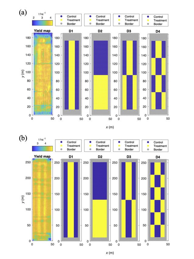
from paddy fields (Fields 1 and 2) were derived from a previous study performed by Zhou et al. (2020) [17] (Figs.1).
The fields were located in Sotohama, Kaizu, Gifu, Japan (35◦ 11’ N, 136◦ 40’ E). The field sizes were 48 × 180 m (~0.86
ha) and 48 × 260 m (~1.25 ha) in Fields 1 and 2 respectively. These fields were remotely sensed by a commercial
multispectral camera (Sequoia+, Parrot, France) mounted on a UAV at the grain-filling stage in 2018 and 2019. Briefly,
winter wheat yield was predicted using a linear regression model with a predictor of enhanced vegetation index 2 (EVI2)
[19] derived from the imagery. The ground sample distance of the imagery was 0.06 m pixel−1 .
Figure 1: The yield map and simulated experimental designs for (a) Field 1 and (b) Field 2. Each yield point indicates
an averaged value within 2.5-m grids. The border points (grey) indicate the area that was not used for the analysis due
to potential edge effects.
3A PREPRINT - M ARCH 16, 2021
Yield monitor data were collected in 2016 at a demonstration farm (Field 3) of New Holland HFT Japan, Inc.
with a commercial combine harvester CX8.70 (New Holland, Belgium) (Fig.2). The field was located in Tomakomai,
Hokkaido, Japan (42◦ 45’ N, 141◦ 44’ E). The entire field size was 8.45 ha, and the area used for the simulation was
100×200 m (2.00 ha). The header width was approximately 5 m, a typical size for a larger-scale farms in Hokkaido. The
yield monitor on the combine harvester recorded the crop yield along harvest transects at an interval of approximately
1.3 m.
Figure 2: The yield map and simulated experimental designs for Field 3. The border points indicate the area that was
not used for the analysis due to potential edge effects.
2.2 Aggregation of yield data
It is not feasible to use raw yield data in linear mixed models due to the high computational cost, particularly for
anisotropic models implemented with a restricted maximum likelihood (REML) estimator (see statistical analysis
section). Interpolated values at a certain grid size are generally used for mapping high-resolution spatial data. For
Fields 1 and 2, the yield map derived from the UAV imagery was averaged within each square grid cell (2.5 × 2.5 m) to
generate mean yield values at the grid centroids. The raw yield monitor data in Field 3 was processed according to
the method proposed by Marchant et al. (2019) [6] with modifications. Briefly, the co-ordinates were rotated as the
combine harvester traveled in the y direction. The x co-ordinates were adjusted across each row in an exact straight
line. Small variations in the co-ordinates and noise in the yield monitor data located near each other may prevent the
estimation of the model parameters. In addition to the method proposed by Marchant et al. (2019) [6], interpolation
was further applied in this study since a square/rectangular lattice of points was preferred to fit the anisotropic model,
as it could accommodate the computational cost and improve the precision of the maximum likelihood calculations.
Therefore, the rotated yield monitor data points were averaged within each rectangular grid cell (2.5 × 5.0 m in the y
and x directions, respectively). For the interval of 2.5 m in the y direction, each averaged yield data point contained 1–2
raw yield data points.
2.3 Simulation of effects on yield of different designs
Two fertilizer treatments (control and treatment plots) were assumed to have been applied in the fields. Treatment plots
received more fertilizer to theoretically increase yield. The experimental design might be very important to reduce
the risk of type I errors and to evaluate the treatment effect precisely. From a practical viewpoint, a tractor equipped
with an 18-m working width broadcaster was assumed to be used for the on-farm experiments, which is equivalent to
3 passes along the long-side direction for Fields 1 and 2 and is equivalent to 5 passes for Field 3. The specifications
of this broadcaster were the same as local farmers’. The edges (15 m from edges associated with turning headlands
and 6 m from edges parallel to field operations) were excluded from the analyses to avoid edge effects in Fields 1
and 2. Four experimental designs were simulated in Field 1 (Fig. 1 a), Field 2 (Fig. 1 b), and Field 3 (Fig. 2). A
simple strip trial (D1) was the easiest and most practical experimental design for farmers. A simple split-plot trial (D2)
was established by splitting the experimental plots perpendicular to the farming operations, and it might require more
complicated manual operation than D1. A combination of strip(s) and split-plot trials (D3) was established. A more
4A PREPRINT - M ARCH 16, 2021
repeated systematic design (D4) was established, which could not be implemented without VRA technology. Note that
the analysis was performed through a simulation study, but the dataset was based on real collected data, which allows
examination of the effect of anisotropy and unpredictable variations in the actual fields.
2.4 Statistical analysis using isotropic and anisotropic spatial linear mixed models
OLS regression is based on the assumption that the errors are independent. In assessing the significance of the treatment
effect on crop yield in on-farm experiments, spatial autocorrelation should be considered because the OLS estimator
increases the risk of type I errors [9, 10]. Thus, a spatial linear mixed model was used to evaluate the effects of
hypothetical treatment on wheat yield. The spatial linear mixed model is written as
y = Xβ + (1)
where y is a vector of length n of the response variable, n is the number of measurements, X is the n × p fixed
design matrix with the values of the vector of size p, which is the number of independent variables, β is a vector of
length p of the fixed-effects coefficients, and is a vector of length n of the random effects with covariance matrix V .
The random effects are assumed to be spatially correlated, and the exponential function was used for the covariance
estimation. The covariance function is written as
c0 + c1 (h = 0)
c(h) = (2)
c1 exp(− ha ) (h > 0)
where c0 is the nugget variance, c1 is the sill variance, h is the distance between the two measurements, and a is
the distance parameter. The theoretical variogram is written as
a
r(h) = c0 + c1 (1 − exp(− )) (3)
h
The above model is a geometrically isotropic model, which has the same parameters in all directions. Marchant et
al. (2019) [6] reported that yield monitor data showed strong anisotropy between the direction of the combine harvester’s
rows and perpendicular to the direction of the rows; thus, a product-sum covariance model [20] was used to model the
variation along each direction. To establish an anisotropic model, direction-specific covariance functions should be
parameterized. The sum-metric model presented by Bilonick (1988) [21] was used in this study. The sum-metric model
is written as
c(hx , hy ) = cx (hx ) + cy (hy ) + cxy (hxy ) (4)
q
hxy = h2x + αh2y (5)
where hx is the lag perpendicular to the farming operation (across rows), hy is the lag in the direction of travel
(within rows), and hxy is the lag obtained by introducing a geometric anisotropy ratio α. The sum-metric model has
been used for fitting space-time variograms previously [22], and its advantage is that the combination of 2-directional
static components and 1 dynamic component of a covariance function is easily interpretable in a physical sense [23].
Thus, the isotropic model has three parameters to be estimated, and the anisotropic model has 8 parameters to be
estimated. For the estimation of these random effects parameters, the REML estimator was used. The REML estimator
does not depend on the unknown fixed effects; therefore, the estimates are less biased than maximum likelihood
estimates [24]. Consequently, the REML estimator calculated the fixed-effect coefficient β and its standard error.
The statistical significance of the experimental treatment was assessed by z statistics, and two-sided p-values were
computed. The preferred model was evaluated based on the lower values of the Akaike information criterion (AIC) [25]
between the geometrically isotropic and anisotropic models. Note that the REML estimator often has a risk of finding a
non-optimum local solution as the optimization solver depends on initial values. Therefore, multiple initial values were
used to iterate the REML estimation although it was computationally demanding. Most of the available applications for
model-based geostatistics, such as the geoR package [26] implemented in the R environment [27], can only fit isotropic
variograms based on the REML estimator. The R package gstat [28] is available for fitting space-time variograms, but
the REML estimator is not implemented. Therefore, it was necessary to develop a user-friendly application that can fit
an anisotropic model based on the REML estimator. All of the computations were conducted using MATLAB [29],
and the documented MATLAB source code is available at GitHub (https://github.com/takashit754/geostat).
5A PREPRINT - M ARCH 16, 2021
Finally, the performances of the three models were compared: OLS regression models, spatial isotropic linear mixed
models, and spatial anisotropic linear mixed models. For the spatial linear mixed models, the residual fitted variograms
were evaluated to check the underlying spatial variations.
2.5 Calculation of type I error rates and estimated accuracy
To assess the estimated model accuracy, randomly generated numbers from a Gaussian distribution (µ=0.3; σ = 0.10 t
ha−1 ) were added to the yield data for each point in the treatment plots. Then, the bias was estimated by computing the
difference between the fixed-effect coefficient β from each statistical model and the population parameter yielded by
a Gaussian random number generator (approximately 0.3 t ha−1 ). In ideal circumstances, on-farm experiments with
multiple treatments in a row achieved the standard error in winter wheat yield of less than 0.05 t ha−1 [6], which was
equivalent to a least significant difference of < 0.1 t ha−1 . The least significant difference ranged from 0.4 to 0.8 t
ha−1 for small-plot field experiments on wheat crops in Japan [30, 31]. It is important to examine whether the small
treatment effect can be detected precisely while avoiding the risk of type I error because such information is crucial to
support the farmers’ management decision. Therefore, the hypothetical treatment effect was intentionally set as the
small value. In addition, 95% confidence intervals were calculated using the standard error estimated from each model.
The simulated type I error rates were presented as p-values of the experimental treatment on the assumption that the
treatment population parameter was zero. To assess the effect of the experimental designs and statistical models on
either the simulated type I error rates or the absolute bias, two-way ANOVA based on type III sums of squares was
performed.
3 Results
3.1 Simulated type I error rates
The effects of the experimental design and model on the simulated type I error rates were evaluated by two-way ANOVA
(Table 1). There was a significant effect of model selection on the simulated type I error rates. There was no significant
interaction between the experimental design and the model. The mean value of the simulated type I error rates was
significantly higher in the anisotropic model than the in OLS model. The simulated type I error rates for each field are
shown in Table 2. The simulated type I error rates were greater than the significance level (>0.05) in the simplest design
(D1) for Field 1 (Table 2). Moreover, they were greater than the significance level (>0.05) in the most repeated and
complicated design (D4) in Fields 2 and 3 (Table 2). Overall, lower simulated type I error rates were more frequently
observed in the OLS model than in the other models. For the anisotropic model, there were no significant simulated
type I error rates for Field 3.
Table 1: Mean values of the simulated type I error rates as affected by experimental design and model.
Type I error rate
Design
D1 0.417
D2 0.396
D3 0.171
D4 0.207
Model
OLS 0.153 b
Isotropic 0.316 ab
Anisotropic 0.425 a
ANOVA
Design n.s.
Model *
Design×Model n.s.
Different small letters indicate significant difference (p < 0.05). *: p < 0.05; n.s.: not significant.
6A PREPRINT - M ARCH 16, 2021
Table 2: The simulated type I error rates for Fields 1, 2, and 3.
Field 1 Field 2 Field 3
Design OLS Isotropic Anisotropic OLS Isotropic Anisotropic OLS Isotropic Anisotropic
model model model model model model model model model
D1 0.17 0.89 0.90A PREPRINT - M ARCH 16, 2021
Figure 3: Bias and 95% confidence intervals in Field 1 (a), Field 2 (b), and Field 3 (c). Iso and Aniso represent the
isotropic and anisotropic models, respectively.
3.3 Residual Variogram Analysis
The 2-directional residual variograms for the estimation of simulated type I error rates in D1 are shown in Fig. 4. In
Field 1, the sill variance in the fitted variogram was 0.036 (t ha−1 )2 in the direction of farming operations (y), while
it was 0.026 (t ha−1 )2 in the direction perpendicular to the farming operations (x). The range parameter that reaches
the sill variance at the 95% level was two times larger in the direction of farming operations (y) (46.1 m) than in the
direction perpendicular to the farming operations (x) (24.1 m). In contrast, in Field 2, the sill variance in the fitted
variogram was approximately 0.034 (t ha−1 )2 in the direction of farming operations (y), while it was 0.027 (t ha−1 )2
in the direction perpendicular to the farming operations (x). The range parameter that reaches the sill variance at the
95% level was 120 m in the direction of farming operations (y), while it was approximately 10 times larger than in the
direction perpendicular to the farming operations (x) (12.3 m). In Field 3, the sill variance in the direction perpendicular
to the farming operations (x) was 2.47 (t ha−1 )2 , and the sill variance in the direction of the farming operations (y)
was 2.87 (t ha−1 )2 . The range parameter that reaches the sill variance at the 95% level was 172 m in the direction of
farming operations (y), while it was approximately 5 times larger than in the direction perpendicular to the farming
operations (x) (31.7 m). Overall, there was strong anisotropy for Field 2 and 3.
Figure 4: The anisotropic experimental and fitted residual variograms for Field 1 (a), Field 2 (b) and Field 3 (c). All
the variograms were computed from the dataset for the estimation of simulated type I error rates in D1. Blue squares
represent experimental variograms in the direction of farming (y). Red circles represent experimental variograms in the
direction perpendicular to the farming operations (x). Experimental semi-variance with more than 30 pairs of identical
lags are displayed. Blue dashed lines indicate fitted variograms in the direction of farming. Red solid lines indicate
fitted variograms in the direction perpendicular to the farming operations.
8A PREPRINT - M ARCH 16, 2021
4 Discussion
Sensor types, data preprocessing, experimental designs, statistical approaches, and within-field spatial structures affect
the precision in on-farm experiments [15, 6]; thus, there are many possibilities for the best experimental design and
statistical approaches in on-farm experiments [2]. Those effects on the type I error rates and estimated accuracy were
explored through a simulation study that generated hypothetical treatments on real wheat yield data in Japanese fields.
Several important implications for experimenters can be drawn from the results.
The experimental designs did not significantly affect the simulated type I error rates although the more repeated
and complicated design (D3 and D4) showed two times smaller simulated type I error rates (Table 1). The results
partially agreed with a previous study, which reported that designs with fewer replications and larger experimental
units tended to increase the risk of type I error [15]. However, the simulated type I error rate was relatively higher
in the simpler design (D1 and D2) than in the other more repeated designs (D3 and D4) in Field 1 (Table 2). This
contradiction may have occurred because the control plots of D3 and D4 coincided with low-yield areas in Field 1
(Fig. 1 a). These results indicated that repeated designs are not sufficient to avoid the risk of type I error. Although
randomization in the repeated designs were not tested in this study, it may contribute to improving the precision of
the experiments as it can accommodate both systematic and erratic spatial trends [32]. The effect of randomization on
the precision of the experiment should be examined in further studies. However, it may not be practical to implement
complex randomization with a variety of treatments in relatively small fields, particularly in Asian countries, even if
VRA technology is available. Moreover, the model was a significant factor affecting the simulated type I error rates
(Table 1). The simulated type I error rates were significantly greater in the anisotropic model than in the OLS model.
Similarly, the more repeated designs and anisotropic models tended to show smaller bias (Table 3), particularly for
Field 3 (Fig. 3), although the effects were not significant. Consequently, the combination of a repeated design and
an anisotropic model might sometimes be a solution for avoiding the risk of type I error and reducing the estimation
bias. However, the isotropic model was able to avoid the risk of type I error for all designs in Field 1 (Table 2). In
this case, the AIC was less in the isotropic model than in the anisotropic model, but only for Field 1 (data not shown).
These results showed that the best model can vary for different fields, according to the experimental design and field
conditions. Therefore, model selection is important for obtaining robust outcomes through on-farm experiments. For
instance, model selection should be carried out to determine whether the anisotropic model is required for analysis of
any specific field.
The fitted residual variograms showed strong anisotropy with different sill variances between the directions for
Field 2 and Field 3 rather than for Field 1 (Fig. 4). The bias was greatly reduced by using an anisotropic model in D2
for Field 3. Furthermore, the anisotropic model had 95% confidence intervals that contained zero for three designs (D1,
D2, and D3), although OLS and isotropic models had 95% confidence intervals that contained zero only for D4 and
D2, respectively. These results are in agreement with the finding from Marchant et al. (2019) [6], who demonstrated
that isotropic models were sufficient for analyzing remotely sensed data but were not appropriate to account for spatial
autocorrelation in yield monitor data. For yield data, they applied a product-sum model [20], which is more complex
than the standard isotropic model. This study demonstrated that the sum-metric model [21] separated the underlying
spatial variation not only from the yield monitor data (Field 3) but also from remotely sensed data (Field 2) to evaluate
the treatment effects more accurately than the isotropic model. Thus, an anisotropic model is sometimes recommended
for the analysis of on-farm data, even data derived from remotely sensed imagery.
In Field 2, experimental variograms indicated that semi-variance was not successfully explained only by lag
distance in the direction perpendicular to the farming operations (x) (Fig. 4). The yield data was noisy and independent
according to the specific rows. This may be attributed not only to the direction of farming operations but also to the
field size, shape or machine capability. Typical Japanese paddy fields are rectangular and small (e.g. less than 1 ha), so
a narrow side may not be sufficiently large to spread fertilizer evenly. For instance, in Fields 1 and 2, the length on the
narrow side was only 48 m, which cannot be divided by the broadcaster’s working width (18 m). As two high-yield lines
were indicated in Field 2 (approximately 15 and 30 m on the x-axis) (Fig. 1 b), some areas may have received fertilizer
application twice, as suggested by Tanaka et al. (2019) [33]. Therefore, small-scale paddy fields may inherently contain
a high variability in the direction perpendicular to the farming operations if the automatic section control system in
the broadcaster or sprayer is not used for on-farm experiments. It is noteworthy that these findings may be specific to
small-scale fields in Asian countries. One solution might be data trimming before statistical analysis if such effects
and errors could be identified from the experimenters’ knowledge. Another solution might be to establish models with
variable intercepts as a random effect for each row. However, the outcomes should be carefully interpreted as the model
becomes complex. Further research is still required to confirm the factors underlying variability in yield and to explore
the best research framework to implement on-farm experiments appropriate for Asian countries with relatively small
fields.
9A PREPRINT - M ARCH 16, 2021
To reiterate, an anisotropic model is an incomplete solution but provides more robust outcomes than traditional
statistical approaches. An anisotropic model is advantageous since it covered larger standard errors when the estimates
had large biases (Fig. 3). Moreover, the 95% confidence intervals of the OLS and isotropic models were generally
narrow, and the hypothetical treatment effects fell outside of them. To make a reliable decision according to the results
of on-farm experiments, experimenters should keep in mind that estimates may not always be precise, but they can
consider how much it could vary, as this variability would result in an adverse scenario. Farmers are not interested
in whether the treatment is significant at the 0.05 level but rather in whether there will be a return on investment [1].
Therefore, as previous studies have determined [34, 10], it is necessary to examine economic feasibility (e.g., marginal
profits) by using real on-farm data in further studies.
5 Conclusions
The outcomes of on-farm experiments can support farmers’ decision-making processes, while inappropriate procedures
will result in incorrect interpretations. The repeated experimental designs examined here did not contribute to reducing
the risk of type I error and bias. Although there are many choices for the experimental design and statistical approaches,
the combination of repeated designs and anisotropic models sometimes provides more reliable outcomes than the
other methods to avoid issues arising from on-farm experiments. The results of the anisotropic model showed large
standard errors, especially when the estimates had large biases. Considering that the aim of on-farm experiments is to
provide farmers with information on economic feasibility, these statistical characteristics of anisotropic models are
advantageous, as experimenters have opportunities to infer the analytical results conservatively. To examine the effect of
these statistical characteristics on farmers’ decision-making processes, economic analysis is needed using real on-farm
data in the future. Overall, this study indicated that the basic framework of on-farm experiments such as experimental
designs and statistical approaches, which has been originally developed in large-scale system, may also be applicable
for small-scale system. However, this simulation study only examined three fields. Further research should be oriented
towards exploring the factors underlying variability in yield and the best research framework to implement on-farm
experiments appropriate for small-scale/smallholder farmers.
Acknowledgments
The authors wish to thank the farming company ’Fukue-eino’ for allowing the survey of their fields and New Holland
HFT Japan, Inc. for providing the yield monitor data. This work was supported by the KAKENHI Early Career
Scientists Grant from the Japan Society for the Promotion of Science (JSPS) (grant number 18K14452) and by the
research grant from the Koshiyama Science and Technology Foundation.
References
[1] Daniel Kindred, Roger Sylvester-Bradley, Sarah Clarke, Susie Roques, Ian Smillie, and Pete Berry. Agronōmics–
an arena for synergy between the science and practice of crop production. In 12th European IFSA Symposium at
Harper Adams University, volume 12, 2016.
[2] Peter M Kyveryga. On-farm research: Experimental approaches, analytical frameworks, case studies, and impact.
Agronomy Journal, 111(6):2633–2635, 2019.
[3] R Sylvester-Bradley. Modelling and mechanisms for the development of agriculture. Aspects of applied biology,
26:55–67, 1991.
[4] DR Hicks, RM van den Heuvel, and Z Fore. Analysis and practical use of information from on-farm strip trials.
Better Crops, 81(3):18–21, 1997.
[5] MJ Pringle, Simon E Cook, and Alex B McBratney. Field-scale experiments for site-specific crop management.
part i: Design considerations. Precision Agriculture, 5(6):617–624, 2004.
[6] Ben Marchant, Sebastian Rudolph, Susie Roques, Daniel Kindred, Vincent Gillingham, Sue Welham, Colin
Coleman, and Roger Sylvester-Bradley. Establishing the precision and robustness of farmers’ crop experiments.
Field crops research, 230:31–45, 2019.
[7] Deborah J Street. Fisher’s contributions to agricultural statistics. Biometrics, pages 937–945, 1990.
[8] M Mzuku, Reich Khosla, R Reich, D Inman, F Smith, and L MacDonald. Spatial variability of measured soil
properties across site-specific management zones. Soil Science Society of America Journal, 69(5):1572–1579,
2005.
10A PREPRINT - M ARCH 16, 2021
[9] Pierre Legendre, Mark RT Dale, Marie-Josée Fortin, Philippe Casgrain, and Jessica Gurevitch. Effects of spatial
structures on the results of field experiments. Ecology, 85(12):3202–3214, 2004.
[10] BM Whelan, JA Taylor, and AB McBratney. A ’small strip’ approach to empirically determining management
class yield response functions and calculating the potential financial ’net wastage’ associated with whole-field
uniform-rate fertiliser application. Field Crops Research, 139:47–56, 2012.
[11] Margareth A Oliver. An overview of geostatistics and precision agriculture. In Geostatistical applications for
precision agriculture, pages 1–34. Springer, 2010.
[12] MJ Pringle, Alex B McBratney, and SE Cook. Field-scale experiments for site-specific crop management. part ii:
A geostatistical analysis. Precision Agriculture, 5(6):625–645, 2004.
[13] DR Kindred, AE Milne, R Webster, BP Marchant, and R Sylvester-Bradley. Exploring the spatial variation in the
fertilizer-nitrogen requirement of wheat within fields. The Journal of Agricultural Science, 153(1):25–41, 2015.
[14] RG Trevisan, DS Bullock, and NF Martin. Spatial variability of crop responses to agronomic inputs in on-farm
precision experimentation. Precision Agriculture, 1–22, 2020.
[15] Carlos Agustín Alesso, Pablo Ariel Cipriotti, Germán Alberto Bollero, and Nicolas Federico Martin. Experimental
designs and estimation methods for on-farm research: A simulation study of corn yields at field scale. Agronomy
Journal, 111(6):2724–2735, 2019.
[16] David S Bullock, Maria Boerngen, Haiying Tao, Bruce Maxwell, Joe D Luck, Luciano Shiratsuchi, Laila Puntel,
and Nicolas F Martin. The data-intensive farm management project: Changing agronomic research through
on-farm precision experimentation. Agronomy Journal, 111(6):2736–2746, 2019.
[17] X Zhou, Y Kono, A Win, T Matsui, and TST Tanaka. Predicting within-field variability in grain yield and
protein content of winter wheat using UAV-based multispectral imagery and machine learning approaches. Plant
Production Science, 1–15, 2020.
[18] L Wang, Y Tian, X Yao, Y Zhu, and W Cao. Predicting grain yield and protein content in wheat by fusing
multi-sensor and multi-temporal remote-sensing images. Field Crops Research, 164:178–188, 2014.
[19] Z Jiang, AR Huete, K Didan, and T Miura. Development of a two-band enhanced vegetation index without a blue
band. Remote Sensing of Environment, 112(10):3833–3845, 2008.
[20] Luigi De Cesare, DE Myers, and D Posa. Estimating and modeling space–time correlation structures. Statistics &
Probability Letters, 51(1):9–14, 2001.
[21] Richard A Bilonick. Monthly hydrogen ion deposition maps for the northeastern us from july 1982 to september
1984. Atmospheric Environment (1967), 22(9):1909–1924, 1988.
[22] JJJC Snepvangers, GBM Heuvelink, and JA Huisman. Soil water content interpolation using spatio-temporal
kriging with external drift. Geoderma, 112(3-4):253–271, 2003.
[23] Gerard BM Heuvelink, P Musters, Edzer J Pebesma, et al. Spatio-temporal kriging of soil water content.
Geostatistics Wollongong, 96:1020–1030, 1997.
[24] Noel Cressie. Statistics for spatial data. John Wiley & Sons, 2015.
[25] Hirotogu Akaike. Information theory and an extension of the maximum likelihood principle. In Selected papers
of hirotugu akaike, pages 199–213. Springer, 1998.
[26] Paulo J Ribeiro Jr, Peter J Diggle, Maintainer Paulo J Ribeiro Jr, and MASS Suggests. The geor package. R news,
1(2):14–18, 2007.
[27] R Core Team et al. R: A language and environment for statistical computing. 2013.
[28] Edzer J Pebesma. Multivariable geostatistics in s: the gstat package. Computers & geosciences, 30(7):683–691,
2004.
[29] MathWorks. Statistics and machine learning toolbox, and global optimization toolbox release 2019b.
[30] H Nakano, S Morita, and O Kusuda. Effect of nitrogen application rate and timing on grain yield and protein
content of the bread wheat cultivar “Minaminokaori” in southwestern Japan. Plant Production Science, 11:151–
157, 2008.
[31] M Okami, H Matsunaka, M Fujita, K Nakamura, and Z Nishio, Z. Analysis of yield-attributing traits for
high-yielding wheat lines in Southwestern Japan. Plant Production Science, 19:360–369, 2016.
[32] HP Piepho, J Möhring, and ER Williams. Why randomize agricultural experiments? Journal of Agronomy and
Crop Science, 199:374–383, 2013.
11A PREPRINT - M ARCH 16, 2021
[33] TST Tanaka, Y Kono, and T Matsui, T. Assessing the spatial variability of winter wheat yield in large-scale paddy
fields of Japan using structural equation modelling. In J. V. Stafford (Ed.) Precision Agriculture ‘19, Proceedings
of the 12th European Conference on Precision Agriculture. Wageningen, The Netherlands: Wageningen Academic
Publishers, pp 751–757, 2019.
[34] Jason Eric Kahabka, HM Van Es, EJ McClenahan, and WJ Cox. Spatial analysis of maize response to nitrogen
fertilizer in central new york. Precision Agriculture, 5(5):463–476, 2004.
12You can also read