Modeling of a split type air conditioner with integrated water heater
←
→
Page content transcription
If your browser does not render page correctly, please read the page content below
Modeling of a split type air conditioner with integrated water heater
                                 P. Techarungpaisan *, S. Theerakulpisut, S. Priprem
       Mechanical Engineering Department, Faculty of Engineering, Khon Kaen University, 123 Mittrapab Rd., Muang, Khon Kaen 40002, Thailand

                               Received 8 April 2005; received in revised form 28 March 2006; accepted 8 October 2006
                                                         Available online 30 November 2006

Abstract

    This paper presents a steady state simulation model to predict the performance of a small split type air conditioner with integrated
water heater. The mathematical model consists of submodels of system components such as evaporator, condenser, compressor, capillary
tube, receiver and water heater. These submodels were built based on fundamental principles of heat transfer, thermodynamics, fluid
mechanics, empirical relationships and manufacturer’s data as necessary. The model was coded into a simulation program and used
to predict system parameters of interest such as hot water temperature, condenser exit air temperature, evaporator exit air temperature,
mass flow rate of refrigerant, heat rejection in the condenser and cooling capacity of the system. The simulation results were compared
with experimental data obtained from an experimental rig built for validating the mathematical model. It was found that the experimen-
tal and simulation results are in good agreement.
Ó 2006 Elsevier Ltd. All rights reserved.

Keywords: Hot water heater; Mathematical model; Model validation; Split type air conditioner; Waste heat

1. Introduction                                                             Thailand and are generally tailor made to the specific
                                                                            requirements of the users. Even though split type air condi-
   In tropical countries such as Thailand, small split type                 tioners with water heaters are successfully used, their per-
air conditioners are generally used in residential and com-                 formance and system design for application in Thailand
mercial buildings. In such establishments, electric water                   have not been fully investigated, especially when both cool-
heaters are often used to generate hot water. Both air con-                 ing and heating effects are desirable. Studies of heat pump
ditioner and electric water heater are generally the major                  hot water heaters operating in subtropical and cold coun-
energy consuming devices in the buildings. The number                       tries have appeared in the literature. Some of such works
of air conditioners and electric water heaters has been                     include those of Ji et al. [1] and Baek et al. [2].
increasing over the years, and this poses a serious problem                    Heat pump and air conditioner models have been widely
to the country that largely depends on imported energy.                     studied. The first heat pump computer model was devel-
Waste heat from air conditioners may be used to produce                     oped by Hiller and Glicksman [3]. A number of models
hot water. The benefits of doing this are two fold. One is                   have been developed and used by researchers and manufac-
elimination of the need to install an electric water heater,                turers. There are also proprietary models that are not avail-
and the other is saving of electrical energy otherwise used                 able for review in the literature. Some of the heat pump
in the electric water heater. These may be accomplished                     models available through the open literature are the
while the usefulness of the air conditioner for cooling is                  MARKIII model developed at a national laboratory by
maintained.                                                                 Fischer et al. [4], the HPSIM model developed at NBS by
   At present, water heaters using waste heat from small                    Domanski and Didion [5] and the heat pump grain drying
split type air conditioners are commercially available in                   models by Theerakulpisut [6]. All of these models are for
                                                                            air-to-air heat pumps. Room air conditioning system mod-
 *
     Corresponding author. Tel.: +66 4535 3382; fax: +66 4535 3333.         eling (RACMOD) developed by Mullen [7] was also avail-
     E-mail address: tec_pisit@yahoo.com (P. Techarungpaisan).              able. This model was based on the governing equations of

0196-8904/$ - see front matter Ó 2006 Elsevier Ltd. All rights reserved.
doi:10.1016/j.enconman.2006.10.012
Nomenclature
A total area (m2) w45 compressor work input (kJ/kg)
C capacity rate (kW/K), capacity rate ratio = swm
w air humidity ratio of saturated air evaluated at
Cmin/Cmax (dimensionless) mean water film temperature (kg water/ kg dry
Cp specific heat (kJ/kg/K) air)
COP coefficient of performance (dimensionless) x refrigerant quality (dimensionless)
DP total pressure drop (kPa)
DPH high side pressure drop (kPa) Greek letters
DPL low side pressure drop (kPa) b thermal expansion coefficient (K1)
DSH degree of superheat (°C) / fin efficiency (dimensionless)
f fraction (dimensionless) e effectiveness of heat exchangers (dimensionless)
g Gravitational acceleration (m/s2) gf electric motor efficiency of rotary compressor
GrD Grashof Number (dimensionless) (dimensionless)
h enthalpy (kJ/kg), heat transfer coefficient gm mechanical efficiency of rotary compressor
(kW/m2/K) (dimensionless)
hasr enthalpy of saturated air evaluated at refrigerant lf dynamic viscosity of saturated refrigerant (Pa.s)
temperature (kJ/kg) m water viscosity (m2/s)
haswm enthalpy of saturated air evaluated at mean p8 eighth pi term (dimensionless)
water film temperature (kJ/kg)
k thermal conductivity (kW/m/K) Subscripts
Le Lewis Number (dimensionless) a air, acceleration
m_ mass flow rate (kg/s) as air side
mw mass of water in hot water tank (kg) c condenser, condensing
N number of transfer units (dimensionless) cap capillary tube
Nud Nusselt Number (dimensionless) comp compressor
P refrigerant pressure (kPa), power (kW) d dehumidification, dew point, dry
PCD compressor discharge pressure (MPa) dsh desuperheating section
PCS compressor suction pressure (MPa) e evaporator, evaporating
Pr Prandtl Number (dimensionless) f saturated liquid, friction
DP pressure drop (kPa) fin fin
q heat transfer rate (kW) g saturated vapour
qhhtp heat rejection rate of heating coil calculated h heating coil
from enthalpy difference between inlet and exit i inlet, inside
of two phase region (kW) ll liquid line
quhtp heat rejection rate of heating coil in two phase m mean
surface evaluated from overall heat transfer max maximum
coefficient equation (kW) min minimum
Ra Rayleigh number (dimensionless) o outlet, outside
t temperature (°C) r refrigerant
tam ambient air temperature (°C) rb return bend
twe water temperature at end of interval of one min- rc receiver
ute (°C) rs refrigerant side
tws water temperature at beginning of interval of sc subcooled section
one minute (°C) sh superheated section
twb wet bulb air temperature (°C) st straight tube
U overall heat transfer coefficient (kW/m2/K) t tube
Uww overall heat transfer coefficient for wet surface tp two phase section
based on enthalpy difference (kg/m2/s) w wet, water
w air humidity ratio (kg water/kg dry air) ws water side
Some of these subscripts are also used in combination. For example, atpo refers to air at outlet of two phase section
and scsta to subcooled liquid, straight tube and component acceleration.the ORNL heat pump model developed by Fisher and Rice
[8] and modified by O’Neal and Penson [9]. All the models
of heat pumps and air conditioners were used to study air-
to-air heat transfer phenomena. None of the aforemen-
tioned models attempted to study the case where waste heat
is to be recovered from the air conditioning system. It is of
great interest to understand the influence of a water heater
addition to the system that performs a dual task of cooling
and heating.
The main objective of this study is to build a reliable
mathematical model of an air conditioner with integrated
hot water heater for the purpose of system study. It is
expected that the model will be sufficiently accurate for
studying the system performance when it is designed to per-
form an extra task of heating water in addition to its nor-
mal cooling task. Parametric study of the system may also
be performed to understand the principal parameters influ-
encing the system performance. The model will be vali-
dated by experimentation to ensure that it may be used
for the intended purpose.
This model was developed from Theerakulpisut’s
model [6]. The difference between this model and The- Fig. 1. Schematic of air conditioner with integrated hot water heater.
erakulpisut’s model lies in the fact that Theerakulpisut’s
model contains reciprocating compressor and thermo-
static expansion valve submodels, whereas this study pro-
poses to model a system that uses a rotary compressor
and a capillary tube. As a result of the inclusion of a
hot water tank between the compressor and the con-
denser, the computer program of this study is also more
complicated since the refrigerant state at the condenser
inlet may be superheated, two phase or subcooled. Mod-
eling of the system is next outlined.
2. Mathematical model
A schematic of the air conditioning system with inte-
grated water heater proposed in this study is shown in
Fig. 1, and its operating cycle is shown in Fig. 2. The sys-
tem consists of the major components of the air condi- Fig. 2. Pressure-enthalpy diagram of vapour compression refrigeration
tioner, namely compressor, evaporator, condenser, cycle.
capillary tube and receiver and an additional water heater
that also serves as a water storage tank. It should be noted
that during normal operation, hot water is expected to be
withdrawn from the tank, and the tank is supplied with capillary tube is assumed to be adiabatic. The entering state
water. At this stage of the study, it is assumed that water of refrigerant can be subcooled or a mixture of liquid and
is not withdrawn from the tank. However, the model will vapour. The effect of coiling the capillary tube is taken into
be further extended to cover the case where hot water is account. This coiling of the capillary tube approximately
withdrawn from the tank. The mathematical model of each reduces the refrigerant mass flow rate by 5% when com-
component can be described as follows. pared with that in a straight tube [11]. Therefore, the eighth
dimensionless pi terms equation is multiplied by 0.95 as
2.1. Capillary tube and compressor model shown in Eq. (1). The procedure for determining p8 may
be found in ASHRAE [10].
The capillary tube model adopts the equation from
m_ r;cap ¼ 0:95p8 d cap lf ð1Þ
ASHRAE [10]. In this method, the Buckingham pi theorem
was applied to the physical factors and fluid properties that The compressor model is obtained by curve fitting the
affect capillary tube flow. The result of this analysis was a manufacturer’s data [12] to give Eq. (2) for the refrigerant
group of eight dimensionless pi terms. The process in the mass flow rate and Eq. (3) for the compressor power input 0:22
1 C rdsh ðt8 tc Þ N dsh
m_ r;comp ¼ 130:12950 1:31674tc þ 0:00696t2c ¼ 1 exp exp CN 0:78 1 ð6Þ
3600
C min ðt8 taci Þ C dsh
þ 9:90989 0:23284tc 0:00194t2c te N dsh C min
fdsh ¼ ð7Þ
þ 0:43826 0:01524tc þ 0:00015t2c t2e ð2Þ U dsh Ac
1 1
P comp ¼ 389:81950 þ 9:84761tc þ 0:06207t2c U dsh ¼ A ð1/Þ
ð8Þ
1000 c
þ has ððAto =Afin Þþ/Þ þ h1as
Ati hrs
þ 18:09224 þ 0:63628tc 0:00332t2c te
The heat transfer rate of the desuperheating section
þ 1:37331 0:06466tc þ 0:00068t2c t2e ð3Þ (qdsh) and the air temperature at the desuperheating zone
Eq. (1) is used to compute the refrigerant mass flow rate exit, which is equal to the air temperature at the two phase
to compare with the value obtained from Eq. (2) until zone inlet (tatpi) are calculated from Eqs. (9) and (10),
agreement within a specified tolerance is achieved. respectively
The work input to the refrigerant during the compres- qdsh ¼ C r ðt8 tc Þ ð9Þ
sion process (w45) can be calculated from Eq. (4). Efficien- tatpi ¼ taci þ qdsh =C a ð10Þ
cies of rotary compressors were given by Ozu and Itami
[13]. Typical mechanical efficiency (gm) and electric motor
efficiency (gf) are both recommended to be 0.85. 2.2.2. Two phase zone
The computation method is the same as that in the the
gm gf P comp desuperheating zone, but the refrigerant side heat transfer
w45 ¼ ð4Þ
m_ r coefficient in the two phase region is evaluated from the
equation proposed by Traviss et al. [16]. The procedure
Then, the refrigerant enthalpy at the compressor exit (h5) for calculating the two phase fraction is as follows:
can be calculated from
etp ¼ 1 eN tp ð11Þ
h5 ¼ h4 þ w45 ð5Þ C a ðtatpo tatpi Þ ðtatpo tatpi Þ
etp ¼ ¼ ð12Þ
where the refrigerant enthalpy at the compressor inlet (h4) C min ðtc tatpi Þ ðtc tatpi Þ
is determined from the receiver model. ftp ¼ Atp =Ac ð13Þ
U tp Atp U tp ftp Ac
N tp ¼ ¼ ð14Þ
2.2. Condenser model C min Ca
By combining Eqs. (11), (12) and (14),
The condenser model consists of a large number of
Ca tc tatpi
equations. Since some of these are quite elaborate, they will ftp ¼ ln ð15Þ
not all be presented here and only the main equations will U tp Ac tc tatpo
be described. Heat transfer in the condenser was modeled Calculation of ftp by Eq. (15) requires tatpo, which can be
using the NTU-e method. The condenser heat transfer area calculated from
is divided into three zones, namely desuperheating, two
tatpo ¼ tatpi þ m_ r hfg =C a ð16Þ
phase and subcooled zones. After leaving the water heater,
the refrigerant entering the condenser can be superheated, Note that Eq. (16) is valid only if the refrigerant enters
two phase or subcooled. Modeling strategy of the con- the two phase section as saturated vapour and leaves as sat-
denser is as follows. urated liquid. The heat transfer rate for the two phase sec-
tion is readily calculated from
2.2.1. Desuperheating zone qtp ¼ m_ r hfg ð17Þ
If the condenser inlet refrigerant state is superheated,
part of the condenser area is in the desuperheating zone. The subcooled zone may exist in the condenser, and the
The Newton–Raphson method is used to solve Eq. (6) for subcooled fraction (fsc) can now be calculated from
the number of transfer unit (Ndsh), and the desuperheat- fsc ¼ 1 ðftp þ fdsh Þ; f tp þ fdsh 6 1 ð18Þ
ing fraction (fdsh) is calculated from Eq. (7). The overall
heat transfer coefficient in the desuperheating zone (Udsh) or f sc ¼ 0 f tp þ fdsh > 1 ð19Þ
is computed from Eq. (8), while the fin efficiency (/) is If the subcooled zone does not exist, i.e. fsc = 0, the two
evaluated from the equation by Charters and The- phase fraction must be determined from
erakulpisut [14]. The refrigerant side heat transfer coeffi-
cient (hrs) is computed from the well known Dittus– ftp ¼ 1 fdsh ð20Þ
Boelter equation, and the air side heat transfer coefficient and the heat transfer rate from
(has) equation is calculated from the equation of Webb
qtp ¼ etp C min ðtc tatpi Þ ð21Þ
[15]The air temperature at the two phase exit (tatpo) is, there- The refrigerant enthalpy at the exit of the two phase sec-
fore, calculated from tion is the enthalpy at saturation corresponding to the pres-
tatpo ¼ tatpi þ qtp =C a ð22Þ sure at the exit of the evaporator (hge), whereas the inlet
refrigerant enthalpy (h2) must be calculated by initially
assuming the refrigerant quality at the inlet (x2). This
2.2.3. Subcooled zone assumed x2 will be later checked as the calculation pro-
If the subcooled fraction is greater than zero, heat trans- ceeds. Once the heat transfer is calculated by Eq. (29),
fer for the subcooled region in the condenser is evaluated the air temperature at the exit of the two phase section
from the following equations. The calculation procedure (tatpo) may be calculated from
is similar to that of the desuperheating section.
tatpo ¼ taei qtp =C a ð30Þ
U sc fsc Ac
N sc ¼ ð23Þ The two phase fraction is computed from Eq. (31) and
C min
0:22 the overall heat transfer coefficient in the dry two phase
N sc 0:78
region (Udtp) is calculated in a similar fashion as in the case
esc ¼ 1 exp exp CN sc 1 ð24Þ
C of the overall heat transfer coefficient in the desuperheating
esc C min ðtc tatpo Þ region of the condenser. The refrigerant side two phase
t9 ¼ tc ð25Þ
C rsc heat transfer coefficient can be computed from the equa-
tion proposed by Chaddock and Noerager [17] and Sthapak
Note that the overall heat transfer coefficient in the sub-
et al. [18].
cooled zone (Usc) takes the same as Eq. (8) used for the
evaluated Udsh. The heat transfer rate for the subcooled Ca taei te
ftp ¼ ln ð31Þ
zone may now be calculated from U dtp Ae tatpo te
qsc ¼ C rsc ðtc t9 Þ ð26Þ It must be remembered that the calculation of (ftp)
and the air temperature at the condenser outlet from according to Eq. (31) is possible because of the initial
assumption of the inlet refrigerant quality (x2), which leads
taco ¼ tatpo þ qsc =C a ð27Þ to the determination of tatpo, which may not necessarily be
The total heat transfer rate in the condenser is simply the correct. The procedure for checking this follows. Once ftp is
sum of the heat transfer rates of the three zones. calculated by Eq. (31), the number of transfer units of the
two phase region (Ntp) is calculated from Eq. (32).
qc ¼ qdsh þ qtp þ qsc ð28Þ
U dtp Atp U dtp ftp Ae
N tp ¼ ¼ ð32Þ
C min Ca
2.3. Evaporator model
and the effectiveness of the two phase section from
Heat transfer area in the evaporator is divided into two etp ¼ 1 eN tp ð33Þ
zones, which are the superheated and two phase zones.
Using the definition of heat exchanger effectiveness, one
2.3.1. Superheated zone may write
Heat transfer in the superheated zone of the evaporator C a ðtaei tatpo Þ ðtaei tatpo Þ
may be calculated from the same equations as were used in etp ¼ ¼ ð34Þ
C min ðtaei te Þ ðtaei te Þ
the desuperheating zone of the condenser.
By equating Eq. (33) and (34), Eq. (35) is obtained for cal-
2.3.2. Two phase zone culating the air temperature at the two phase zone exit of
It will be assumed that dehumidification may take place the evaporator (tatpo).
only on the two phase surface. This assumption can be tatpo ¼ taei ðtaei te Þð1 eN tp Þ ð35Þ
checked by comparing the calculated air dew point and
the calculated mean fin temperature at the interface Eq. (35) may now be used to calculate tatpo using the Ntp
between the two phase and the superheated zones. In fact, previously calculated from Eq. (32). This new tatpo is then
the two phase surface may be entirely dry, partially wet or used in Eq. (30) to calculate qtp. The new value of qtp is
totally wet, depending on the incoming air condition. then substituted into Eq. (29) to calculate h2, which is used
to calculate the new x2. The new x2 is then compared with
2.3.2.1. Entirely dry two phase surface. If the air tempera- the initially assumed value. If they do not agree within a
ture passing through the evaporator is higher than its specified tolerance, the new x2 is used to begin the next
dew point, it is not dehumidifying. Therefore, the heat loop of iteration until the desired agreement is achieved.
transfer is evaluated in the entirely dry two phase surface Once the actual operating cycle is established, the evap-
condition as Eq. (29) orator exit air temperature may be obtained from
qtp ¼ m_ r ðhge h2 Þ ð29Þ taeo ¼ tatpo qsh =C a ð36Þwhere qsh is Ca taei te
fdtp ¼ ln ð43Þ
qsh ¼ C r ðDSHÞ ð37Þ U dtp Ae tad te
The degree of superheat (DSH) was experimentally The wet two phase surface fraction (fwtp) is then given by
obtained for the system in this investigation. The values fwtp ¼ 1 fsh fdtp ð44Þ
of DSH varied from 1.66 to 1.97 °C, therefore the average
DSH of 1.8 °C is used in the model. It is important to note that the dry surface fraction (fdtp) is
The total heat transfer in the evaporator for the entirely zero when the two phase fraction is entirely wet and that
dry two phase surface condition is evaluated from Eq. (38). Eq. (44) still holds.
The heat transfer rate from the air to the refrigerant in
qe ¼ qtp þ qsh ð38Þ the dry two phase section may be calculated from
So far, the evaporator has been modeled on the assump- qdtp ¼ C a ðtaei tad Þ ð45Þ
tion of an entirely dry evaporator surface. However, this is
rarely the case under normal operating conditions. It is, The method for analyzing the wet evaporator in this
therefore, necessary to determine whether there is dehu- study is adopted from Threlkeld [19]. The method was used
midification of water vapour on the evaporator coil. The by Theerakulpisut and Priprem [20], and it was found that
criteria for establishing this will be outlined next. it accurately predicted the performance of wet evaporator
surfaces. The method is quite complicated and involves a
2.3.2.2. Two phase surface with dehumidification. In the number of equations. For the purpose of outlining the cal-
evaporator, dehumidification begins at the location where culation procedure, only the principal equations of the
the mean fin temperature is equal to the dew point of the methods are presented as follows.
incoming air (td). Thus, the air temperature at the location The humidity ratio change across the wet surface may be
where dehumidification just begins (tad) is computed from calculated from
Eq. (39). 1
dw ha haswm
td /ð1 U dtp Ae =hrs Atei Þte ¼ Le þ ðhwg 2501LeÞ ð46Þ
tad ¼ ð39Þ dha ww swm
1 /ð1 U dtp Ae =hrs Atei Þ
where
Eq. (39) may be used to calculate tad which is then com-
pared with the air temperature at the exit of the two phase hwg ¼ 2501 þ 1:805w ð47Þ
section (tatpo) calculated from Eq. (35). If tatpo is greater The complexity of Eq. (46) lies in the method for cal-
than tad, the whole two phase surface is dry, and the mod- culating the mean value of the mean water film tempera-
eling approach is as presented in Section 2.3.2.1. If tatpo is ture for evaluating haswm and w swm . The procedure for
less than tad, the two phase section is partially or entirely establishing this was outlined by Theerakulpisut and Pri-
wet. It can be further established whether the surface is prem [20].
entirely wet by comparing tad with the air temperature at Consideration of Eq. (46) reveals that an analytical solu-
the evaporator inlet (taei). If taei is less than tad, the whole tion is difficult and numerical integration is deemed appro-
surface is wet, otherwise it is partially wet. priate. By substituting all the terms pertaining to the inlet
The Newton–Raphson method is used to solve Eq. (40) condition of the wet section of the evaporator, dh dw
is
a i
for the number of transfer units of the superheated region evaluated. As an approximation, one may write
(Nsh) assuming a value of tatpo in Eq. (40), which must be
Dw wei wtpo dw
checked later for agreement with the new value calculated ¼ ¼ ð48Þ
from the analysis of the two-phase section. Then the super- Dha had hatpo dha i
heated fraction (fsh) and the two phase fraction (ftp) are which gives
computed from Eqs. (41) and (42), respectively
0:22 dw
C r ðt3 te Þ N sh wtpo ¼ wei ðhad hatpo Þ ð49Þ
¼ 1 exp 0:78
exp CN sh 1 dha i
C min ðtatpo te Þ C
where
ð40Þ
N sh C min had ¼ tad þ wei ð2501 þ 1:805tad Þ ð50Þ
fsh ¼ ð41Þ
U sh Ae It can be shown that the enthalpy of the air at the outlet
ftp ¼ 1 fsh ð42Þ section of the two phase section is given by
If the two phase surface is determined by the previously hatpo ¼ hasr þ ðhad hasr ÞeU ww fwtp Ae =m_ a ð51Þ
discussed criterion to be partially wet, further division of
the surface into dry and wet two phase sections is neces- Now, it is possible to predict the air temperature at the out-
sary. From the definition of heat exchanger effectiveness let of the two phase section
and the effectiveness equation similar to Eq. (33), the dry
two phase fraction takes the following form: tatpo ¼ ðhatpo 2501wtpo Þ=ð1 þ 1:805wtpo Þ ð52ÞThe heat transfer rate in the two phase section may now be 2.6.1. Pressure drops in the evaporator, the condenser and
calculated from the heating coil
qtp ¼ m_ a ðhaei hatpo Þ ð53Þ There are six components of the pressure drop in the
evaporator, which are evaluated from Eq. (60).
Hence, the total heat transfer rate of the evaporator is
DP e ¼ ðDP tpstf þ DP tpsta Þ þ DP tprbf þ ðDP shstf þ DP shsta Þ þ DP shrbf
given by
ð60Þ
qe ¼ qtp þ qsh ð54Þ
The straight tube two phase pressure drop can be calcu-
The refrigerant enthalpy at the inlet of the evaporator (h2) lated by using the relationship proposed by Traviss et al.
can be calculated from [16] and the return bend two phase pressure drop by the
h2 ¼ h3 qe =m_ r ð55Þ relationship given by Geary [21]. While the straight tube
single phase pressure drop can be computed from the well
The new refrigerant quality x2 is calculated from Eq. (56)
known Darcy-Weisbach equation [10], the return bend sin-
and compared with the assumed value
gle phase pressure drop makes use of the relationship pro-
x2 ¼ ðh2 hfe Þ=ðhge hfe Þ ð56Þ posed by Ito [22].
If the new x2 does not agree with the assumed value, the Pressure drop in the condenser is similarly calculated by
new value is used in the next round of iteration. This pro- Eq. (61). It should be noted that there are additional pres-
cedure is repeated until x2 converges to a specified sure drop components because the equation must also
tolerance. cover pressure drops in the subcooled zone. This equation
is also used to compute pressure drops in the heating coil in
the water tank.
2.4. Liquid, suction and discharge lines
DP c ¼ ðDP tpstf þ DP tpsta Þ þ DP tprbf þ ðDP shstf þ DP shsta Þ
Heat transfer in the liquid, suction and discharge lines þ DP shrbf þ ðDP scstf þ DP scsta Þ þ DP scrbf ð61Þ
can be evaluated in the form of free convection. For exam-
ple, heat loss from the refrigerant in the liquid line to ambi-
ent air is calculated from 2.6.2. Pressure drops in the connecting pipes
Single phase pressure drops in the connecting pipes are
dqll ¼ U ll ðtr tam ÞdAll ¼ m_ r C pr dtr ð57Þ
evaluated by the Darcy-Weisbach equation. When the con-
which can be integrated to give the refrigerant temperature necting pipes contain two phase fluid, the pressure drop is
at the outlet of the liquid line as calculated in a similar manner as in the case of the two
t1 ¼ tam þ ðt9 tam Þ expðU ll All =m_ r C pr Þ ð58Þ phase pressure drop in the evaporator.
It should be mentioned that the connecting pipe between
2.7. Refrigerant properties
the hot water tank and the condenser is assumed to be insu-
lated. Therefore, the heat transfer in this connecting pipe is
The refrigerant in the air conditioner in this study is R-
negligible. The refrigerant temperature at the heating coil
22. Thermodynamic properties of the refrigerant are evalu-
exit (t7) is equal to the refrigerant temperature at the con-
ated by the equations presented by Cleland [23]. The phys-
denser inlet (t8).
ical properties are calculated from equations obtained by
curve fitting the data of ASHRAE [10] and the equations
2.5. Receiver model
presented by Stoecker and Jones [24].
The receiver model is assumed to be under a steady state
condition, and there is no insulation. The receiver may be 2.8. Water heater model
considered as a container of vapour receiving heat from
the environment. In this condition, sensible heat will be The water tank, which contains a heating coil, is located
added to the vapour refrigerant by natural convection from between the condenser and the compressor. Heat transfer
the ambient air. Thus, on the refrigerant side is divided into three zones as shown
in Fig. 3.
m_ r C pr ðt30 t4 Þ ¼ hrc Arc ðtrm tam Þ ð59Þ
The refrigerant state at the heating coil inlet, state 6, is
where the refrigerant temperature at the receiver inlet ðt30 Þ determined from the discharge line model. All of the
is evaluated from the suction line model. heating coil is first assumed to be a desuperheating sur-
face. The desuperheating section of the heating coil area
(Ahdsh) is equal to the total heating coil area (Ah). The
2.6. Pressure drop in the system
refrigerant temperature at the heating coil exit (t7) is cal-
culated from
Pressure drop in the system consists of pressure drops in
the major components of the system and connecting pipes. t7 ¼ twm þ ðt6 twm Þ expðU hdsh Ahdsh =m_ r C pr Þ ð62Þand the desuperheating area of the heating coil (Ahdsh) can
be calculated from
m_ r C pr tc twm
Ahdsh ¼ ln ð71Þ
U hdsh t6 twm
Then, it is assumed that all of the remaining area is a two
phase surface
Ahtp ¼ Ah Ahdsh ð72Þ
The exit refrigerant quality of the heating coil (x7) is as-
sumed in order to calculate the overall heat transfer coeffi-
cient in the two phase region (Uhtp). Then, the heat
Fig. 3. Schematic of a heating coil. rejection rate in the two phase section of the heating coil,
which is evaluated from Eq. (73), is compared with the heat
where twm is the mean water temperature over a period of rejection rate calculated from the enthalpy difference be-
one minute (°C). This value is first assumed and will be cal- tween the inlet and the exit of the two phase region, Eq.
culated later. (74)
The overall heat transfer coefficient in the desuperheat-
ing section in the heating coil (Uhdsh) can be evaluated from quhtp ¼ U htp Ahtp ðtc twm Þ ð73Þ
Eq. (63). qhhtp ¼ m_ r ðhgc h7 Þ ð74Þ
1 where the refrigerant enthalpy at the heating coil exit (h7)
U hdsh ¼ ð63Þ
ho =d hi Þ
d ho
d hi hrs
þ d ho lnðd
2k h
þ h1ws can be evaluated from
The refrigerant side convective heat transfer coefficient h7 ¼ hfc þ x7 hfg ð75Þ
in the heating coil (hrs) is evaluated by the same correla- If the values of quhtp and qhhtp do not agree within an
tions as used in the desuperheating section of the con- acceptable tolerance, x7 is varied, and Uhtp, quhtp and qhhtp
denser. The water side convective heat transfer coefficient are recalculated until the desired agreement between quhtp
(hws) is computed from the equations proposed by Chur- and qhhtp is achieved. During the procedure to compare
chill and Chu [25]. quhtp and qhhtp, if h7 is less than the enthalpy of saturated
0 1
liquid refrigerant at the condenser pressure (hfc), the sub-
B 0:518Rað1=4Þ C cooled zone may exist. In this case, the heat transfer rate
NuD ¼ 0:36 þ @ ð9=16Þ ð4=9Þ A
106 < Ra < 109
1 þ 0:559 of the two phase section of the heating coil (qhtp) can be
Pr
calculated from
ð64Þ
0 0 112 qhtp ¼ m_ r hfg ð76Þ
B B 0:387Rað1=6Þ CC 5 12 Then, the heat transfer area of the two phase section of the
NuD ¼ @0:6 þ @ 0:559ð9=16Þ ð8=27Þ AA 10 < Ra < 10
1 þ Pr heating coil (Ahtp) is evaluated from
qhtp
ð65Þ Ahtp ¼ ð77Þ
U htp ðtc twm Þ
hws d ho
NuD ¼ ¼ Nusselt Number ð66Þ
k The subcooled area of the heating coil (Ahsc) may now be
Ra ¼ GrD Pr ¼ Rayleigh Number ð67Þ calculated from
gbðtr twm Þd 3h;out Ahsc ¼ Ah Ahdsh Ahtp ð78Þ
GrD ¼ ¼ Grashof Number ð68Þ
m2
The refrigerant temperature at the exit of the heating coil at
If t7 calculated from Eq. (62) is greater than the con- (t7) is calculated from
densing temperature corresponding to the condenser pres-
sure (tc), the whole area of the heating coil is t7 ¼ twm þ ðtc twm Þ expðU hsc Ahsc =m_ r C pr Þ ð79Þ
desuperheating. So, the heat transfer rate in the heating coil Therefore, the heat transfer rate of the subcooled section of
can be calculated from the heating coil (qhsc) can be calculated from
qhdsh ¼ m_ r ðh6 h7 Þ ð69Þ
qhsc ¼ m_ r ðhfc h7 Þ ð80Þ
If t7 is less than tc, two phase and subcooled zones may
During the calculational procedure to establish the
also exist in the heating coil. In this case, the heat rejection
agreement between quhtp and qhhtp, if h7 is greater than
in the desuperheating zone (qhdsh) is calculated from
hfc, the subcooled section does not exist. Therefore,
qhdsh ¼ m_ r ðh6 hgc Þ ð70Þ qhsc = 0, t7 = tc and qhtp is evaluated fromqhtp ¼ m_ r ðhgc h7 Þ ð81Þ capillary tube inlet refrigerant temperature (t1,new) is then
compared with the assumed value. If they do not agree
The total heat transfer rate in the heating coil is simply the within a specified tolerance, the new value of capillary tube
sum of the heat transfer rates of the three zones inlet temperature will be used to repeat the calculation pro-
qh ¼ qhdsh þ qhtp þ qhsc ð82Þ cess until convergence is achieved. The calculation proce-
dure may now go to the evaporator subroutine. From the
It should be noted that the mean water temperature knowledge of the refrigerant state at the outlet of the evap-
(twm) is first assumed at the beginning of the calculation orator, state 3, and by assuming the evaporator inlet air
procedure, the new value of mean water temperature condition, the evaporator subroutine is used to calculate
(twm,new)will be calculated from Eq. (84). If the twm,new does refrigerant state 2. Once state 2 is determined, the enthalpy
not agree with the assumed value, the new value is used in at this state (h2) is compared with the enthalpy at the inlet
the next round of iteration. This procedure is repeated until of the capillary tube (h1). If they do not agree within the
twm converges to a specified tolerance. specified tolerance, the evaporator inlet air temperature is
qh x60 varied until the desired agreement between h1 and h2 is
twe ¼ tws þ ð83Þ achieved. Once, this is established, the vapour refrigerant
mw C pw
cycle is established for some evaporator inlet air tempera-
tws þ twe ture. This inlet air temperature is compared with the actual
twm;new ¼ ð84Þ
2 evaporator inlet air temperature. If they do not agree
within a specified tolerance, the exit evaporator pressure
P3 is changed to a new value and the whole calculation pro-
3. Model simulation program cedure is repeated until the calculated evaporator inlet air
temperature agree with the actual value. Then, the refriger-
The mathematical model is coded into a computer pro- ant state at the capillary tube inlet must be checked. If h1 is
gram using FORTRAN 90. This simulation program can greater than hfc, the refrigerant state at the capillary tube
be used to calculate parameters of prime interest such as inlet is two phase. Therefore, the refrigerant quality at
water temperature in the hot water tank, condenser exit the capillary tube inlet (x1) is computed, and the program
air temperature, evaporator exit air temperature, refriger- will proceed to then compare with the assumed value. If
ant mass flow rate, heat rejection in the condenser and in they do not agree within a specified tolerance, the x1,new
the hot water tank and cooling capacity of the system. will be used to repeat the calculation process until conver-
All dimensions of the system components such as fin and gence is achieved.
tube geometry of the evaporator and the condenser, dimen- It should be noted that in the first loop of analysis, the
sions of the capillary tube, and dimensions of the connect- pressure drops across all components of the system are
ing pipes are included in the program. The input data of assumed to be negligible so that P1 may be taken as P5,
the program are the initial water temperature and the and P2 as P3. The effects of pressure drops may now be
degrees of superheat of the refrigerant at the evaporator taken into account to improve the analysis as illustrated
exit. in Fig. 4.
To begin simulation, the program reads the first set of At this point, simulation of the model has been finished
operating condition data, i.e. the air dry bulb and wet bulb for the first set of operating condition data. The program
temperatures at the evaporator inlet and the air dry bulb then reads the second set and the operating condition data
temperature at the condenser inlet. The evaporator exit from the input data file and proceeds in a similar manner
pressure (P3), compressor discharge pressure (P5), high side until the end of the simulation.
pressure drop (DPH) and low side pressure drop (DPL) are
first assumed. The capillary tube inlet refrigerant tempera- 4. Model validation
ture (t1) is initially assumed to be less than the saturated
refrigerant temperature corresponding to the condenser An experimental rig of an air conditioning system with
pressure (tc), and therefore, the refrigerant state is assumed integrated water heater was built for the purpose of verify-
to be subcooled at the capillary tube inlet. Then, the refrig- ing the model. Basically, the experimental rig consists of six
erant mass flow rate ðm_ r;cap Þ is computed by the capillary major components of the system, namely compressor,
tube model and compared with the refrigerant mass flow receiver, evaporator, condenser, capillary tube and a water
rate ðm_ r;comp Þ, which is calculated from the rotary compres- heater. The schematic of the experimental set up is shown
sor model. If they do not agree within an acceptable toler- in Fig. 5. The hot water tank is located between the com-
ance, P5 will be changed according to the scheme shown in pressor and the condenser. Note that in this arrangement,
Fig. 4, and the refrigerant mass flow rate will be recalcu- water in the hot water tank is not withdrawn while being
lated until the agreement between m_ r;cap and m_ r;comp is estab- heated. This configuration represents the situation where
lished. The program proceeds according to the flow chart hot water is produced and stored for later use. It also rep-
to evaluate refrigerant states 3 0 , 4, 5, 6, 7 and 9. The value resents the simplest and least expensive arrangement if
of t1 is calculated from the liquid line subroutine. The new waste heat from the air conditioner is to be used for heatingInput initial water temperature tw, DSH
Open input data file (*.txt) Read taei,actual , twb aei,t aci
Assumed P3 ,P5 ,t1 ,taei ,DPH=0, DPL=0, x1=0
Capillary tube model, compute mr,cap
Compressor model, compute Pcomp ,w45, m r, comp
mr,cap >m r,comp? m =m ?
r,cap r,comp
P5=P5-0.01kPa
Yes No
P5=P5+0.01kPa Ye s
No
Suction line model, compute state 3'
Receiver model, compute state 4
Compute state 5, h5=h4+w45
Discharge line model, compute state 6
Heating coil in hot water tank subroutine,
compute state 7,t 7, qh
Condenser subroutine, compute state 9, qc, taco
Liquid line model, compute state 1, t1,new
t1,new = t1 ?
t1=t1,new
No
Ye s
Evaporator subroutine, compute state 2, qe , taeo
Change taei h2= h1 ?
No
Ye s
Change P3 No taei= taei,actul ?
Compute quality Yes
x1 = x1,new of refrigerant at h1 > hfc ?
cap.tube inlet
No x1,new = x1 ? x1,new= (h1-hfc)/ Yes
(hgc-hfc) No
Yes
Pressure drop model, compute pressure drops in all
components and compute DPHnew,DPLnew
DP=abs(DPHnew+DPLnew-DPH-DPL)
(DPH = DPHnew)
DP < 2 kPa ? No (DPL=DPLnew )
Ye s
Compute water temperature tW,new , COP of System
Open output data file (*.txt)
Record the required output parameter
Is the end of input data file?
No min=min+1
tw=tw,new
Ye s
END
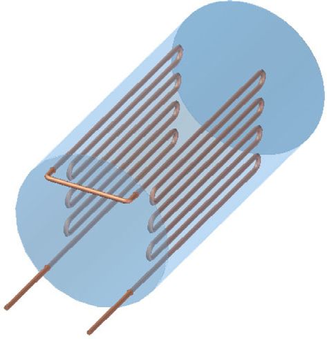
Fig. 4. Flow chart of the simulation program of a split type air conditioner with integrated water heater.the total length of 10.6 m. The hot water tank is insulated
with 50.8 mm synthetic rubber insulation.
5. Measuring equipment
The experimental rig was equipped with measuring
equipment to determine the refrigerant and air states,
power inputs, refrigerant and air mass flow rates and hot
water temperature.
5.1. Temperature measurement
As indicated in Fig. 5, temperature measurements are
made by K-type thermocouples at sixteen locations, three
locations (t4, t5, t9) for refrigerant temperatures, four loca-
tions (t14 t17) for air dry bulb and air wet bulb air tem-
peratures at the inlet and the exit of the evaporator and
one location (t18) for air dry bulb air temperature at the
condenser inlet, four locations (t19 t22) for air dry bulb
temperatures at the condenser exit and four locations
(t10 t13) for the water temperature in the hot water tank.
All the thermocouples were calibrated with a GRANT
water bath with an accuracy of ±0.5 °C (5–90 °C) and con-
nected to the CAMBELL model CX-23 data logger inter-
faced with a desk top computer.
Note that the condenser exit air temperature was mea-
Fig. 5. Schematic of measuring positions in the experiment.
sured at four different positions, and therefore, the con-
denser exit temperature was taken as the average value
of these four positions. Similarly, the water temperature
water. The cooling capacity of the air conditioner is in the hot water tank was also taken as the average value
12,000 Btu/h (3.517 kW), while the hot water tank capacity of four readings at four different positions within the
is 102 l. The heating coil in the hot water tank consists of tank.
two similar coils as shown in Fig. 6. The coil is made from It should also be noted that in measuring the air wet
copper tubing with 1.27 mm diameter. Each heating coil bulb temperatures, the thermocouples were covered with
consists of six straight tubes each with a length of wicks that were fed with distilled water from bottles
0.59 m., two straight tubes that are 0.635 m. in length through plastic tubes leading to the wicks. The feed rate
and 7 U-bends with 25 mm radius with a total length of of water was experimentally determined to avoid excessive
5.3 m. The two coils were connected in series, thus having addition of water to the air system. Wet bulb readings
were verified by a brand new Testo model 625 having
an accuracy ±0.5 °C (10 to 60 °C). Since these thermo-
couples were placed in the air stream through the evapo-
rator with sufficient air velocity, the wet bulb readings
were quite accurate provided that the wicks were suffi-
ciently wet.
Refrigerant temperatures were also measured by K-type
thermocouples. The thermocouples were installed on the
outside surface of the copper tubes and thermal paste
was applied to ensure good contact between the thermo-
couples and the tube surface.
5.2. Refrigerant pressure measurement
Refrigerant pressures were measured at five locations
(P2, P4, P5, P7, P9) by Bourdon pressure gauges. These
pressure gauges were new and factory calibrated with an
Fig. 6. Heating coil in the water tank. accuracy of ±1% of full scale.5.3. Refrigerant mass flow rate 7. Results and discussion
The refrigerant mass flow rate was measured by a HED- For the purpose of validating the mathematical model,
LINE orifice type model HLIT-205-2G flow meter with an ten experimental runs to cover a wide range of operating
accuracy of ±2% of full scale. This flow meter is intended conditions were conducted, and important parameters were
for single liquid phase measurement, so it was installed in recorded for comparison with the simulation results. These
the liquid line. A sight glass was installed before the flow parameters include compressor exit refrigerant tempera-
meter to ensure that the refrigerant was in liquid phase ture, evaporator exit air temperature, condenser exit air
when readings were taken. temperature, compressor discharge and suction pressures,
refrigerant mass flow rate and compressor power input.
The actual operating conditions of the experiments, as
5.4. Air flow rate determined by the inlet conditions of the air flow through
the evaporator, the inlet air temperature through the con-
Air flow rates through the condenser and the evapora- denser and the initial water temperature in the hot water
tor were measured by measuring air velocities at the exits tank, were used to simulate the model. The simulation
of the condenser and the evaporator. The air velocities results of all the ten runs were found to be in good agree-
were measured by a Testo model 425 anemometer with ment with the experimental results. Thus, only the simula-
telescopic probe. The anemometer has an accuracy of tion and experimental results of a typical experimental run
±0.05 m/s (0–20 m/s). Before taking measurements, the will be present.
fan speed of the evaporator was set at the highest speed. Typical experimental and simulation results are pre-
The air velocities for the condenser and the evaporator sented in Figs. 7–15. Fig. 7 compared predicted and exper-
were taken at ten different locations. The average values imental temperatures of refrigerant at the compressor exit.
of these ten locations were used in calculation of the air Except for the first ten minutes of the experiment, this fig-
mass flow rates through the condenser and the evapora- ure reveals that the model overpredicted the experimental
tor. Since the experimental rig was run with fixed con- data by 9%. Figs. 8 and 9 show plots of experimental
denser and evaporator fan speeds, the air mass flow and predicted values of the evaporator exit air temperature
rates were determined only once for every experimental and the condenser exit air temperature. The percentage
run. deviations of the experimental values from the predicted
values were 4% for the evaporator exit air temperature
5.5. Power input measurement and 3% for the condenser exit air temperature.
As indicated in Fig. 10, the experimental compressor
The power input to the system was measured by a discharge and suction pressures deviated from the pre-
FLUKE 39 power meter with an accuracy of ±2% dicted values within ±5%. The experimental and predicted
(0–10 kW). The meter was new and factory calibrated. refrigerant mass flow rates are shown in Fig. 11, and the
experimental and predicted compressor power inputs are
shown in Fig. 12. Fig. 11 reveals that the model overpre-
6. Experimental procedure dicted the experimental data by 6%, whereas Fig. 12 indi-
cates that the model underpredicted the experimental
Before each experimental run, the data logger and the value by 7%.
computer were turned on to check that all the measuring Fig. 13 compares experimental and predicted water tem-
instruments were ready for the experiment. Initial operat- peratures in the hot water tank. This figure reveals that the
ing condition, as defined by the air dry bulb and wet bulb model overpredicted the experimental data by approxi-
temperatures at the evaporator inlet, the air dry bulb tem- mately 7% during the first hour of the experiment and that
perature at the condenser inlet and the initial water temper- agreement between the experimental and predicted values
ature in the water tank, were recorded. Once the were very good after that.
experimental rig was turned on, thermocouple readings Figs. 14 and 15 present experimental data and predicted
were recorded in a data file at intervals of one minute. values for heat rejection rates at the condenser and cooling
The recorded data included the operating conditions, capacity of the evaporator, respectively. The percentage
which were used for the model simulation, as well as other deviations from the predicted value were ±24% for the con-
parameters for model validation. During the course of a denser heat rejection rate and ±21% for the cooling capac-
preliminary run of the experiment, it was found that refrig- ity of the evaporator. It should be noted that the condenser
erant pressures, refrigerant mass flow rate and power heat rejection rate, and the cooling capacity are derived
inputs were almost constant. These parameters were, there- quantities. Equipment errors in the measurement of air
fore, recorded at an interval of ten minutes. Since the temperature and humidity can contribute to significant
experiment was mainly for the purpose of model valida- errors of the quantities. An error analysis was conducted
tion, a period of three hours for each experimental run to determine the greatest possible errors from the calcula-
was judged to be sufficient. tion of these two quantities. The method of analysis as100
90
Compressor exit refrigerant
80
70
temperature (˚C) 60
50
40
30
20
t5(Predicted)
10 t5(Experimental)
0
5 15 25 35 45 55 65 75 85 95 105 115 125 135 145 155 165 175
Time (min)
Fig. 7. Predicted and experimental compressor exit refrigerant temperatures.
20
taeo(Predicted)
18 taeo(Experimental)
Exit air temperature (˚C)
16
14
12
10
8
6
5 15 25 35 45 55 65 75 85 95 105 115 125 135 145 155 165 175
Time (min)
Fig. 8. Predicted and experimental evaporator exit air temperatures.
40
38
Exit air temperature (˚C)
36
34
32
taco(Predicted)
taco(Experimental)
30
5 15 25 35 45 55 65 75 85 95 105 115 125 135 145 155 165 175
Time (min)
Fig. 9. Predicted and experimental condenser exit air temperatures.3
PCD (Predicted)
PCD (Experimental)
PCS (Predicted)
Re frigerant pressure (MPa)
PCS(Experimental)
2
1
0
10 20 30 40 50 60 70 80 90 100 110 120 130 140 150 160 170 180
Time (min)
Fig. 10. Predicted and experimental compressor discharge and suction pressures.
0.05
mr (Predicted)
mr (Experimental)
0.04
Mass flow rates (kg/s)
0.03
0.02
0.01
0
10 20 30 40 50 60 70 80 90 100 110 120 130 140 150 160 170 180
Time (min)
Fig. 11. Predicted and experimental refrigerant mass flow rates.
2.0
Power (Predicted)
Power (Experimental)
Compressor power input (kW)
1.5
1.0
0.5
0.0
10 20 30 40 50 60 70 80 90 100 110 120 130 140 150 160 170 180
Time (min)
Fig. 12. Predicted and experimental compressor power inputs.50
40
Water temperature (˚C)
30
tw (Predicted)
tw (Experimental)
20
5 15 25 35 45 55 65 75 85 95 105 115 125 135 145 155 165 175
Time (min)
Fig. 13. Predicted and experimental water temperatures in the hot water tank.
6
Heat rejection rates at the condenser (kW)
5
4
3
2
1 qc (Predicted)
qc (Experimental)
0
5 15 25 35 45 55 65 75 85 95 105 115 125 135 145 155 165 175
Time (min)
Fig. 14. Predicted and experimental heat rejection rates at the condenser.
6
5
Cooling capacity (kW)
4
3
2
1 qe (Predicted)
qe (Experimental)
0
0 15 25 35 45 55 65 75 85 95 105 110 115 125 135 155 165 175
Time (min)
Fig. 15. Predicted and experimental cooling capacities of the evaporator.described in Ref. [26] was based on a careful specification [4] Fisher SK, Rice CK, Jackson WL. The Oak Ridge heat pump design
of the uncertainties in the various primary experimental model: MARK III version program documentation. Report No.
ORNL/TM-10192. Oak Ridge National Laboratory; 1988.
measurements. It was found that the greatest possible [5] Domanski P, Didion D. Computer modeling of the vapor compres-
errors were ±24.37% for the condenser heat rejection rate sion cycle with constant flow area expansion device. Report No. NBS
and ±24.58% for the evaporator cooling rate. These errors BSS 155, NBS, 1983.
were, therefore, comparable with the actual discrepancies [6] Theerakulpisut S. Modelling heat pump grain drying systems. PhD
between the experimental and simulation values. thesis. The University of Melbourne, Australia, 1990.
[7] Mullen CE. Room air conditioner system modeling. M.S. Thesis, The
University of Illinois at Urbana-Champaign, USA, 1994.
8. Conclusions [8] Fisher SK, Rice CK. The Oak Ridge heat pump models: I. A steady-
state computer design model for air-to-air heat pumps. Report No.
A mathematical model of a split-type air conditioner ORNL/CON-80/R1, Oak Ridge, TN, Oak Ridge National Labora-
with integrated water heater has been developed by tory, 1983.
detailed modeling of the system components. The model [9] O’Neal DL, Penson SB. An analysis of efficiency improvement in
room air conditioner. ESL/88-04, Texas A&M University; 1988.
is based on the fundamental principles of thermodynamics, [10] ASHRAE Handbook, Fundamental, CD-Rom 1997.
heat transfer and fluid mechanics. Empirical equations are [11] Kuehl SJ, Goldschmidt VW. Steady flows of R-22 through capillary
used to describe the heat and mass transfer and pressure tubes: test data. ASHRAE Trans 1996;104:719–28.
losses occurring in these components. The principle advan- [12] Siam Compressor Industry Co., Ltd. Specification for compressor.
tages of the model based on this approach are that the Thailand, 2002.
[13] Ozu M, Itami T. Efficiency analysis of power consumption in small
model provides flexibility for design changes and that the hermetic refrigerant rotary compressors. Int J Refrig
model can be expected to reflect the real behavior of 1981;4(5):265–70.
the system, as evidenced from the experimental and pre- [14] Charters WWS, Theerakulpisut S. Efficiency equations for constant
dicted results in this study. The model was validated thickness annular fins. Int Commun Heat Mass Transfer
against experimental data, and it was found that the model 1989;16(4):547–58.
[15] Webb RL. Air-side heat transfer correlations for flat and wavy plate
is quite accurate in predicting important system parame- fin-and-tube geometries. ASHRAE Trans 1990;96:445–9.
ters. The model will be further used to study the perfor- [16] Traviss DP, Rohsenow WM, Baron AB. Forced convection conden-
mance of other system configurations under different sation inside tubes: a heat transfer equation for condenser design.
operating conditions. Parametric study of different systems ASHRAE Trans 1973;79(1):157–65.
may also be performed to understand the principal param- [17] Chaddock JB, Noerager JA. Evaporation of R-12 in a horizontal
tube with constant wall heat flux. ASHRAE Trans 1966;72(1):
eters influencing the system performance. 90–102.
[18] Sthapak BK, Varma HK, Gupta CP. Heat transfer coefficients in dry-
Acknowledgement out region of the horizontal tube water heated R-12 evaporator.
ASHRAE Trans 1976;87(2):1087–104.
This study was supported financially by the Energy Pol- [19] Threlkeld JL. Thermal environmental engineering. Prentice-Hall Inc;
icy and Planning Office (EPPO), Ministry of Energy, Thai- 1972.
[20] Theerakulpisut S, Priprem S. Modeling cooling coils. Int Commun
land and the Energy Management and Conservation Office Heat Mass Transfer 1998;25(1):127–37.
(EMCO), Khon Kaen University, Thailand. [21] Geary DF. Return bend and pressure drop in refrigeration system.
ASHRAE Trans 1975;8(1):250–64.
References [22] Ito H. Pressure losses in smooth pipe bends. J Basic Eng
1960:131–43.
[1] Ji Jei, Chow Tin-tai, Pei Gang, Dong Jun, He Wei. Domestic air- [23] Cleland AC. Computer subroutines for rapid evaluation of refriger-
conditioner and integrated water heater for subtropical climate. Appl ant thermodynamic properties. Int J Refrig 1986;9:346–51.
Therm Eng 2003;23:581–92. [24] Stoecker WF, Jones JW. Refrigeration & Air Conditioning. Singa-
[2] Baek NC, Shin UC, Yoon JH. A study on the design and analysis of a pore: McGraw-hill International Edition; 1982.
heat pump heating system using wastewater as a heat source. Solar [25] Churchill SW, Chu HHS. Correlating equations for laminar and
Energy 2005;78(3):427–40. turbulent free convection from a horizontal cylinder. Int J Heat Mass
[3] Hiller CC, Glicksman LR. Improving heat pump performance via Transfer 1975;18:1049–53.
compressor capacity control-analysis and test. Energy Laboratory [26] Holman JP. Experimental Methods for Engineers. 7th ed. Singa-
Report No. MIT-EL 76-001, vols. I and II. MIT, 1976. pore: McGraw-Hill International Edition; 2001.You can also read