A Model of Ice Wedge Polygon Drainage in Changing Arctic Terrain - MDPI
←
→
Page content transcription
If your browser does not render page correctly, please read the page content below
water
Communication
A Model of Ice Wedge Polygon Drainage in Changing
Arctic Terrain
Vitaly A. Zlotnik 1 , Dylan R. Harp 2 , Elchin E. Jafarov 2        and Charles J. Abolt 2, *
 1   Department of Earth and Atmospheric Sciences, University of Nebraska-Lincoln, Lincoln, NE 68588, USA;
     vzlotnik1@unl.edu
 2   Earth and Environmental Sciences Division, Los Alamos National Laboratory, Los Alamos, NM 87545, USA;
     dharp@lanl.gov (D.R.H.); elchin@lanl.gov (E.E.J.)
 *   Correspondence: cabolt@lanl.gov

 Received: 25 September 2020; Accepted: 25 November 2020; Published: 1 December 2020

 Abstract: As ice wedge degradation and the inundation of polygonal troughs become increasingly
 common processes across the Arctic, lateral export of water from polygonal soils may represent an
 important mechanism for the mobilization of dissolved organic carbon and other solutes. However,
 drainage from ice wedge polygons is poorly understood. We constructed a model which uses
 cross-sectional flow nets to define flow paths of meltwater through the active layer of an inundated
 low-centered polygon towards the trough. The model includes the effects of evaporation and
 simulates the depletion of ponded water in the polygon center during the thaw season. In most
 simulations, we discovered a strong hydrodynamic edge effect: only a small fraction of the polygon
 volume near the rim area is flushed by the drainage at relatively high velocities, suggesting that
 nearly all advective transport of solutes, heat, and soil particles is confined to this zone. Estimates of
 characteristic drainage times from the polygon center are consistent with published field observations.

 Keywords: ice wedge; thermokarst; active layer; flow net

1. Introduction
     Polygonal tundra landscapes have experienced rapid change in recent decades. Across the
Arctic, an abrupt acceleration in ice wedge degradation has been observed since the second half of
the twentieth century [1–3]. This melting results in a deepening of troughs at polygon boundaries,
which often become inundated. The formation and expansion of flooded troughs, or thermokarst
pools (hereafter referred to as trough pools, for short), has profound influence on tundra hydrology
and ecological processes. For example, in polygonal terrain with poorly developed (undegraded)
troughs, hydrologic simulations suggest that most fluxes of water into and out of the active layer are
vertical, either in the form of precipitation or evapotranspiration [2]. After troughs deepen, however,
observations indicate that water may drain laterally from the active layer of the polygon interior
throughout the summer [4–8]. A common result of this drainage is the flushing of nutrients and other
solutes from polygonal soils into trough pools, where they may fertilize plant growth [7]. This flushing
may be especially effective at mobilizing dissolved organic carbon, because exposure to sunlight
following the discharge of water from tundra soils commonly accelerates oxidation [9].
     Given the importance of this transition to tundra hydrology and carbon cycling, a number of
studies have begun to incorporate ice wedge degradation into land surface models [10–13]. However,
to our knowledge, very little work offers insights into the dynamics of active layer drainage at the
scale of individual polygons (~10 m). Here, we present a three-dimensional axisymmetric transient
model of the flow above and inside an inundated low-centered polygon surrounded by flooded
troughs, resulting in a simple analytical solution. Within our model, all subsurface flow occurs within

Water 2020, 12, 3376; doi:10.3390/w12123376                                     www.mdpi.com/journal/water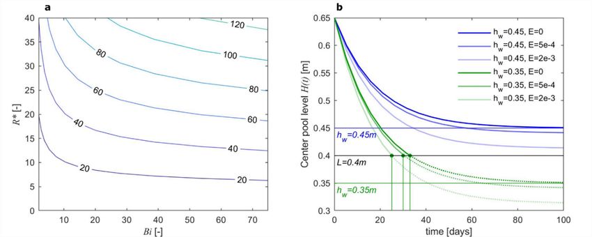
Water 2020,12,
Water 2020, 12,3376
x FOR PEER REVIEW 22 of 14
14
a seasonally thawed layer which, depending on the time within the thaw season, is equal to or less
athick
seasonally
than thethawed
activelayer
layer,which, depending
here defined on portion
as the the timeofwithin the thaw season,
the subsurface is equal to or
which experiences less
phase
thick than the active layer, here defined as the portion of the subsurface which
change between ice and liquid water [14]. Typically, the thickness of this thawed layer follows a experiences phase
change
roughlybetween ice and
asymptotic liquid water
trajectory, [14]. Typically,
increasing quickly atthe thethickness
start of ofthethissummer,
thawed layer follows a
then gradually
roughly asymptotic trajectory, increasing quickly at the start of the summer, then
stabilizing near the active layer thickness late in the season. Accordingly, we studied an idealized gradually stabilizing
near the active
(cylindrical) layer thickness
low-centered late inwith
polygon, the aseason. Accordingly,
seasonally thawed depthwe studied
L, andan idealized
a radial (cylindrical)
distance R from
low-centered polygon, with a seasonally thawed depth L, and a radial distance
the center point to the interior wall of the rims; the depth L can either be treated as constant R from the center point
for
to the interior wall of the rims; the depth L can either be treated as constant
simulations of short time duration, or changed dynamically, using numerical or analytical for simulations of short
time duration,Our
approaches. or changed dynamically,
model includes using numerical
the effects or analytical
of the polygon approaches.
geometry, anisotropy,Our and
model includes
hydrologic
the effects of the polygon geometry, anisotropy, and hydrologic interconnection
interconnection between the polygon center and the trough, with consideration of evaporation. between the polygon
centerParameterized
and the trough,bywith consideration
published of evaporation.
field data from polygonal soils, the model indicates that water
movement in the active layer occurs predominantlypolygonal
Parameterized by published field data from soils, the
at the periphery model
of the indicates
polygon center,that water
while the
movement in the active layer occurs predominantly at the periphery of the polygon
interior conducts very little water. Hence, advective flushing of mass, solutes, and energy is confined center, while the
interior
primarily conducts very
to a small little at
region water. Hence,
the edge advective
of the polygon.flushing of mass, solutes, and energy is confined
primarily to a small region at the edge of the polygon.
2. Conceptual Model
2. Conceptual Model
We consider a three-dimensional axisymmetric transient model of the flow in an inundated,
We consider a three-dimensional axisymmetric transient model of the flow in an inundated,
cylindrical, low-centered polygon in which a thermokarst pool had begun to develop, characterized
cylindrical, low-centered polygon in which a thermokarst pool had begun to develop, characterized by
by a thawed layer of depth L, and a distance R from the center point of the polygon to the start of the
a thawed layer of depth L, and a distance R from the center point of the polygon to the start of the rim
rim (Figure 1). Pools of water exist both in the center and in the trough.
(Figure 1). Pools of water exist both in the center and in the trough.
Figure 1. Schematic diagram of our three-dimensional axisymmetric analytical model of inundated
Figure 1. Schematic
low-centered diagram
polygon of our
drainage. three-dimensional
The axisymmetric
diagram represents analytical
an idealized model of
“pie wedge” inundated
section of a
low-centered polygon drainage. The diagram represents an idealized
low-centered polygon, including pools in the center and trough. “pie wedge” section of a low-
centered polygon, including pools in the center and trough.
In cylindrical coordinates (r, z), the vertical z-axis is directed downward from the polygon surface
whileInr iscylindrical coordinateswhich
the radial coordinate, ( , ),isthe
zerovertical -axis iscenter.
at the polygon directedThedownward
datum for the from the polygon
hydraulic head
surface while r is the radial coordinate, which is zero at the polygon center.
is located at the base of the thawed layer. The pool has a uniform water level, H (t), which reduces The datum for the
hydraulic
over time t,head
and is
is located at the
constrained basespilling
from of the thawed
by a rimlayer. The pool
separating has a uniform
the center from thewater (Figure( 1).
troughlevel, ),
which reduces over time t, and is constrained from spilling by a
The water level in the trough with respect to the datum, hw , is treated as constant. rim separating the center from the
trough (Figure of
Drainage 1).water
The water
throughlevelthe
in the trough
active layerwith respect
of the to thecenter
polygon datum,toward
hw, is treated as constant.
the trough pool is
Drainage
controlled of waterresistance,
by hydraulic through which
the active layer of on
is dependent thehorizontal
polygon and center toward
vertical the trough
hydraulic pool is
conductivity
controlled by hydraulic resistance, which is dependent on horizontal
(Kr and Kz , respectively), polygon size, and the hydraulic exchange rate between the polygon and and vertical hydraulic
conductivity
trough. ( and
The latter , respectively),
is defined by hydraulicpolygon
resistance size, andpolygon–trough
of the the hydraulic exchange
interface. rate
This between
resistancethe
is
apolygon
functionand trough. The
of interface latter lisand
thickness defined by hydraulic
hydraulic conductivityresistance
k. Withoffiner
the sediments
polygon–troughon the interface.
interface,
Thiscan
one assumeiska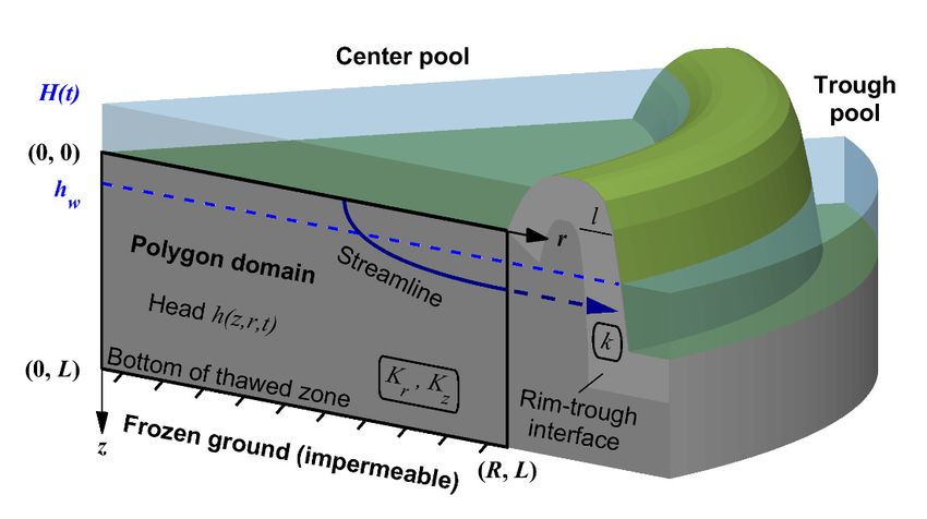
Water 2020, 12, 3376                                                                                3 of 14

the rim, which may be in the order of several meters [15]. Thus, the flux across the polygon boundary
(r = R) at each elevation is defined by the difference between the head in the trough (hw ) and the
head in the polygon subsurface across from the trough at this elevation, h(R, z, t). In general, the flux
direction may vary.
     The value d = H (0) − hw represents the initial head difference that drives the drainage.
The drainage completion time, tdrain , is defined by the equation H (tdrain ) = L.
     Hydraulic head inside of the active layer, h(r, z, t), responds rapidly to the center pool level at
the surface (H(t)) due to the small vertical scale of the active layer. The polygon thickness L(t) may
vary from zero to a maximum value of D and can be scaled as follows: L(t) = D·f (t), where f(t) is a
dimensionless function that varies from 0 to 1 by the end of the season. The thickness of the thawed
layer can also be treated as constant for qualitative analyses or simulations of a short time duration.

3. Methods

3.1. Problem Statement For Constant Thaw Depth
     In this case, L = D, a constant. Due to the small vertical scale of the polygon, soil compressibility
effects on the flow of water through the active layer are neglected in the following flow equation:

                            Kr ∂ ∂h       ∂2 h
                                    !
                                 r    + Kz 2 = 0, 0 < r < R, 0 < z < L                                 (1)
                            r ∂r ∂r       ∂z

      The boundary condition at the z-axis indicates axial symmetry as follows:

                                         ∂h(0, z, t)
                                                     = 0, 0 < z < L                                    (2)
                                            ∂r

      The boundary condition at the surface is defined by the pool level H (t):

                                       h(r, 0, t) = H (t),           0 < r < R                         (3)

     Exchange of water across the polygon interior/trough interface (i.e., under the rim) can be described
using a Robin boundary condition that relates flux to the difference in head at each elevation between
the radial boundary and the trough, through the coefficient κ:

                              ∂h(R, z, t)
                       − Kr               = κ[h(R, z, t) − hw ],          κ ≈ k/l,    0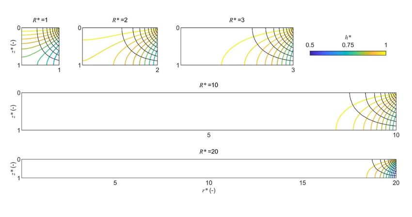
Water 2020, 12, 3376                                                                                                                       4 of 14

3.2. Reduction to Dimensionless Steady-State Problem
      We introduce new dimensionless coordinates for space (r∗ , z∗ ) and time (t∗ ) as follows:
                                                               r
                                                 ∗     r             Kz                    z                    t
                                             r       =                  ,         z∗ =       ,        t∗ =                                    (7)
                                                       L             Kr                    L                   tL

and define functions for head h∗ (r∗ , z∗ ) in the thawed zone and center pool depth H∗ (t∗ ):

                                                              h(r, z, t) − hw                                 H (t) − hw
                                  h∗ (r∗ , z∗ ) =                             ,            H∗ (t∗ ) =                                         (8)
                                                               H (t) − hw                                      H0 − h w

with dimensionless parameters:

                                                                                               R∗
                                                                                                    ∂h∗ (r∗ , 0) ∗ ∗
                       r
                                                             κL
                                                                                       Z
           ∗     R         Kz            ∗                                    ∗                                                  E·tL
         R     =              ,     Bi       =           √           ,    Q        =                            r dr ,   E∗ =                 (9)
                 L         Kr                                Kr Kz                         0           ∂z∗                      H0 − h w

where the dimensional parameter tL below represents a characteristic drainage time of the model:

                                                                                     R2
                                                                         tL =                                                               (10)
                                                                                   2Kr L·Q∗

     These substitutions replace time-dependent h(r, z, t) by the time-independent dimensionless
function h∗ (r∗ , z∗ ). The time dependence is embedded in H∗ (t∗ ) by Equation (8):

                  h(r, z, t) = [H (t) − hw ]·h∗ (r∗ , z∗ ) + hw ,                              H (t) = (H0 − hw )·H∗ (t∗ ) + hw             (11)

    This transformation relies on the assumption that head inside the thawed zone responds rapidly to
changes in the level of the center pool. The resulting boundary value problem for h∗ (r∗ , z∗ ) is as follows:

                            1 ∂ ∗ ∂h∗                         ∂2 h ∗
                                                     !
                                  r                      +                = 0,         0 < r∗ < R∗ , 0 < z∗ < 1                             (12)
                            r∗ ∂r∗ ∂r∗                        ∂z∗ 2

                                                         ∂h∗ (0, z∗ )
                                                                      = 0,                 0 < z∗ < 1                                       (13)
                                                            ∂r∗
                                                     h∗ (r∗ , 0)         = 1,          0 ≤ r∗ ≤ R∗                                          (14)
                                                 ∂h∗ (R∗ , z∗ )
                                             −                  = Bi·h∗ (R∗ , z∗ ),                      0 < z∗ < 1                         (15)
                                                     ∂r∗
                                    ∂h∗ (r∗ , L)
                                                 = 0, 0 < r∗ < R∗                                                                           (16)
                                       ∂z∗
      The dimensionless form of the water balance Equation (6) with initial conditions is:

                                                     dH∗
                                                         = −H∗ − E∗ ,                    H ∗ (0) = 1                                        (17)
                                                     dt∗
      This equation explains drainage for the duration 0 < t < tdrain .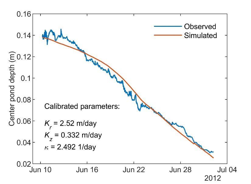
Water 2020, 12, 3376                                                                                         5 of 14

3.3. Solutions

3.3.1. Head h*(r*, z*)
    The solution of the boundary value problem (12)–(16) for h∗ (r∗ , z∗ ) can be found by the standard
method of separation of variables. Details are presented in Appendix A.
                                           X∞                     J0 (λn r∗ )           cosh(λn (1 − z))
                       h∗ (r∗ , z∗ ) = 2                                                                      (18)
                                                                       λn                  cosh(λn )
                                                                  h                 i
                                              n=1
                                                      λn R J0 (λn R ) Bi + J1 (λn R )
                                                          ∗        ∗               ∗

where λn , n = 1, 2, . . . are roots of the equation.

                                           λn J1 (λn R∗ ) = Bi·J0 (λn R∗ ), n = 1, 2, . . .                   (19)

      Values of h∗ (r∗ , z∗ ) range from 0 to 1.

3.3.2. Fluxes and Stokes Stream Function ψ*(r*, z*)
     One variable of primary interest is the transient drainage rate, Q(t), which can be calculated using
the dimensional parameters and variables in Equations (7) and (8):

                                                          R
                                                              ∂h(r, 0, t)
                                                  Z
                             Q(t) = −2πKz                                 rdr = −2πKr L[H (t) − hw ]·Q∗       (20)
                                                      0          ∂z

where the time-independent constant Q∗ was defined in Equation (9). Using Equations (18) and (19),
one obtains:
                                                X∞        tanh(λn )
                          Q∗ = Q∗ (R∗ , Bi) = 2            2                             (21)
                                                  n=1
                                                        λn λBin + 1

       The axial symmetry of the flow permits effective analysis of the kinematic flow structure inside
the polygon using the time-independent Stokes stream function, ψ∗ (r∗ , z∗ ). This function is related to
h∗ (r∗ , z∗ ) by conditions of orthogonality of their gradients:

                                                 ∂ψ∗     ∗ ∂h
                                                             ∗                ∂ψ∗     ∗ ∂h
                                                                                          ∗
                                                     ≡ −r      ,                  ≡ r                         (22)
                                                 ∂r∗       ∂z∗                ∂z∗       ∂r∗
subject to the condition:
                                                                   ψ∗ (0, 0) = 0                              (23)

       The latter equation indicates zero flux at the intersection of the polygon surface (z = 0) and the
symmetry axis. Level curves of the function ψ∗ (r∗ , z∗ ) are perpendicular to the equipotentials of head
h∗ (r∗ , z∗ ) for isotropic hydraulic conductivity conditions, which satisfies the Laplace equation at any
moment in time. The flow net of streamlines and equipotentials provides a tool for visualizing the
flow structure inside the thawed zone.
       Using Equations (7), (8), (22), and (23), one obtains:
                                                          R r∗∂h∗ (r∗ ,z∗ ) ∗ ∗
                                     ψ∗ (r∗ , z∗ ) =          0  ∂z∗
                                                                           r dr
                                                                  J1 (λn r∗ )r∗             sinh(λn (1−z))    (24)
                                     =2 ∞
                                          P
                                                                        λ
                                              n=1                                              cosh(λn )
                                                           h                              i
                                                      λn R∗ J0 (λn R∗ ) Bin + J1 (λn R∗ )

    The maximal value of ψ∗ (r∗ , z∗ ) is located at the point z = 0 and r = R. The normalized dimensionless
Stokes stream function varies between 0 and 1:

                                                                    ψ∗ (r∗ , z∗ )         ψ∗ (r∗ , z∗ )
                                       Ψ∗ (r∗ , z∗ ) =                                =                       (25)
                                                                  max ψ∗ (r∗ , z∗ )       ψ∗ (R∗ , 0)
Water 2020, 12, 3376                                                                                                        6 of 14

where
                                                            ψ∗ (R∗ , 0) = Q∗                                                 (26)

     Importantly, the positions of streamlines based on the dimensional and dimensionless normalized
stream functions do not depend on time, but the flux magnitude does change over time, as defined in
Equation (20).

3.3.3. Center Pool Level H(t): Constant Thaw Depth
      The solution of the initial value problem (17) for depth H*(t*) is:

                             H (t) − hw                 ∗           ∗                                             t
                                        = H∗ (t∗ ) = e−t − E∗ 1 − e−t ,                             t∗ =                     (27)
                              H0 − h w                                                                             tL

     At large time values, this equation shows that the stabilized water level in the pool, Hmin , is equal
to or below the water level in the trough if hw remains constant:

                                               limH (t) = Hmin = hw − E·tL                                                   (28)
                                                    t→∞

     In the case of non-zero evaporation from the center pool, the drainage may become reversed, i.e.,
the trough with constant water level hw may become a source of water for the center pool.
     The center pool will not be drained entirely, if

                                                    Hmin = hw − E·tL > L                                                     (29)

      In other cases Hmin can decrease to the elevation of the polygon surface and satisfy the condition
H (tdrain ) = L. In this case, the time of complete pool drainage continues from Equation (27) as follows:

                                                                                  H0 − L

                                               tdrain = tL ln 1 +                                                            (30)
                                                                               L − hw + EtL

3.3.4. Center Pool Level H(t): Dynamic Thaw Depth, Analytical Approach
    In this case, L(t) = D·f(t), and the problem requires treatment of a moving bottom boundary, which
requires additional effort. Equation (6) is amended by using the relationship in Equation (20):

                                  dH
                            πR2      = −2πKr L[H (t) − hw ]·Q∗ − πR2 E,                           H ( 0 ) = H0               (31)
                                  dt
     Which can be rewritten for integration considering the definitions of t* and H* in Equations (7)
and (8) as follows:
                               dH∗
                                     = −p(t∗ )H∗ − E∗ , H∗ (0) = 1                              (32)
                                dt∗
     The time-dependent coefficient p(t*) here is as follows:

                                                                      2Kr (H0 − hw ) f Q∗
                                                 p(t∗ ) =                                                                    (33)
                                                                             R2
     Which reflects a time-dependent, experimentally determined function f for the active layer.
Transient f also creates time dependence in the parameters R* and Q* in Equation (9). Finally,
integration of the linear Equation (32) is standard:
                                                            Z    t∗                                   Z       t∗
                        ∗   ∗        −P(t∗ )      −P(t∗ )                 P(η) ∗              ∗
                       H (t ) = e              −e                     e      E (η)dη,   P(t ) =                    p(ξ)dξ    (34)
                                                             0                                            0
Water 2020, 12, 3376 7 of 14
3.3.5. Center Pool Level H(t): Dynamic Thaw Depth, Numerical Approach
As an alternative to the methods described in Section 3.3.4, dynamic seasonally thawed zone
thickness can also be accounted for by solving the model in a piecewise fashion, dividing the time
domain into discrete timesteps. In this approach, the thawed zone thickness L(t) is represented in
table format and treated as forcing data for each timestep. Additionally, this approach permits head in
the trough pool to likewise be defined in table format as a function of time, hw (t). An example using
this approach to simulate the early-summer disappearance of a center pond near Utqiagvik, Alaska is
presented in Section 4.3.
3.4. Computation of Solutions
Scripts for these calculations have been provided in the Supplementary Material. The methods
used to investigate pool dynamics are determined by whether the thaw depth is treated as constant
or dynamic.
When the thaw-layer thickness L is steady, a constant value of R* is defined. Flow net calculations
start with determining a set of λn , n = 1, 2, . . . in Equation (19). Convergence of the series in
Equations (18) and (24) is generally rapid. Next, the dimensionless head is converted to dimensional
format by Equation (11), and constant, dimensionless flux Q* is calculated using specific R∗ and Bi by
Equation (21). This Q* is utilized in estimates of tL and pool depth dynamics, by Equations (10) or (27).
Geometric and soil physical parameters are defined in the opening lines of the scripts and can easily be
manipulated by the user. An example of this model is presented in Section 4.2.
When thaw-layer thickness L is dynamic, the function f must be known a priori in analytical
or table format. The value of R* becomes time dependent according to Equation (33) because of the
continuously changing polygon radius-to-depth ratio. Corresponding λn , n = 1, 2, . . . differ for each
moment of time, together with Q* according to Equation (21). If the function f is not provided as a
continuous function, Equation (32) can be solved using a finite-difference approach on a discrete time
grid, as described in Sections 3.5.2 and 4.3.
3.5. Model Parameters for Demonstration
3.5.1. Constant Thaw-Layer Thickness
To demonstrate the use of the model under assumptions of constant thaw-layer thickness, we used
ranges for geometric and soil physical parameters of ice-wedge polygons derived from the literature.
Based on ice-wedge polygon horizontal scale and vertical thickness from [2,7,16,17], we explored
aspect ratios (R/L) ranging from 1 to 20.
Our hydraulic conductivity values are derived from [18], who analyzed peat cores and determined
heterogeneous Kr in the range between 0.1 and 10 m/day, but typically on the order of 1 m/day.
The anisotropy ratio Kr /Kz had somewhat erratic behavior, often appearing nearly isotropic, but
with a range extending from 0.1 and 10. Similar values for hydraulic conductivity were published
by [4,7,16,19,20], but these studies generally did not distinguish between Kr and Kz . Estimates by [8]
for high-centered and low-centered polygons had generally similar magnitudes of Kr .
Higher values of Kr and Kz are sometimes observed immediately in the top 0.2–0.3 m (relative to
the underlying part of the active layer) by one or two orders of magnitude [16,18]. This scenario may
effectively increase the initial effective pool depth and reduce the thickness of the active layer, but will
not affect concepts of the model.
For characteristic cases, the maximum center pool depth in low-centered polygons, H0 , can be
taken in the order of 0.5 m [2,5,15].
3.5.2. Dynamic Thaw-Layer Thickness
In order to validate the model in a scenario characterized by dynamic thaw-layer thickness,
we calibrated it to match ponded water levels in a low-centered polygon during an early seasonWater 2020, 12, 3376 8 of 14
drainage event in 2012 at the Barrow Environmental Observatory near Utqiagvik, Alaska (Area A in [5]).
We used measured data from the site as boundary conditions for the model, including directly observed
trough water levels. Meteorological forcing data consisted of observed precipitation from the Barrow,
Alaska National Weather Service ground station and re-analyzed evapotranspiration from NASA’s
Global Land Data Assimilation System (GLDAS) [21]. Although the thaw depth was not measured
directly in the polygon during the 2012 thaw season, it was measured directly during the 2013 and
2014 thaw seasons. Using the 2013 and 2014 thaw depth measurements and atmospheric conditions,
we calibrated a permafrost heat flow model (Geophysical Institute Permafrost Laboratory (GIPL)
model) [22] and simulated thaw depths for 2012 using air temperature and snow depth measured at
the site. We applied these simulated thaw depths to control the dynamic thaw depth of the model.
In order to incorporate varying precipitation, evapotranspiration, trough water level, and thaw
depth, we ran the model in piecewise fashion, restarting the model at each timestep with current
boundary conditions. We included data from 6:00 AM, June 10 through 6:00 AM, July 2, 2012 (23 days)
during which time the inundated low-centered polygon drained. The data was collected every 15 min,
resulting in 2112 timesteps in the analysis.
The adjustable parameters in the calibration were the horizontal and vertical hydraulic conductivity
(Kr and Kz ), the discharge conductance (κ), and the initial ponded water level (H(0)). We calibrated
the model using a Levenberg–Marquardt approach implemented in the Julia LsqFit package (https:
//github.com/JuliaNLSolvers/LsqFit.jl). The objective function was the sum of the squared errors
between the measured and simulated ponded water levels in the polygon center. Regularization terms
were added to the objective function to penalize solutions where Kr and κ deviated from physical
values. Assuming preferential horizontal (radial) flow, the value of Kz was required to be less than Kr .
4. Results
4.1. Flow Nets: Head and Flux Distributions
To assess the effects of aspect ratio R/L on flow dynamics, we assumed isotropic conditions
(Kr = Kz ), and the coefficient κ = 2.0 day−1 (assuming k as a fraction of Kr (e.g., 50%) and l on
the order of 0.25 m). For a polygon L = D = 0.5 m thick, several horizontal polygon sizes were
considered: R =0.5, 1.0, 1.5, 5.0, and 10.0 m. q
√ κL 2·0.5 R Kz
The dimensionless parameters are as follows: Bi =
Kr Kz
= √ = 1 and R∗ = L Kr =
√ 1·1
R
0.5 1 = 1, 2, 3, 10, and 20 (Figure 2). The latter two values correspond to commonly observed ice-wedge
polygon radii of around 5–10 m. For comparison, the smaller aspect ratios of R∗ = 1, 2, and 3 are also
shown, to highlight the impact of disparity between radial and vertical scales.
The shape of the flow net is steady during the drainage period, while the magnitude of each
local velocity vector declines with the depth of water in the center pool, as defined in Equation (20).
Considering that each stream tube conducts identical discharge toward the periphery of the polygon,
the flux magnitudes near the polygon center and the trough differ by orders of magnitude.
These results indicate that the primary flux region is focused within about two vertical scales
from the rim, when aspect ratio is approximately 3.0 or greater. This water flux disparity implies that
advection-driven transport of solutes, heat, and soil particles may be concentrated near the periphery
of an inundated polygon, while the center remains poorly flushed.
An investigation of model sensitivity to other contributing factors (hydraulic resistance of
polygon-trough interface and anisotropy for commonly observed values) indicated that they are
secondary to the effect of aspect ratio; these results are discussed in Appendix B.Water 2020, 12, x FOR PEER REVIEW 9 of 14
An investigation of model sensitivity to other contributing factors (hydraulic resistance of
polygon-trough interface and anisotropy for commonly observed values) indicated that they are
secondary to the effect of aspect ratio; these results are discussed in Appendix B.
Water 2020, 12, 3376 9 of 14
Figure 2. Effects of variable R* on the spatial distribution of fluxes across the polygon. The color
bar applies to the head h∗ (r∗ , z∗ ). All streamlines (in black) are contour lines of the stream function
ΨFigure
∗ (r∗ , z∗ ), defining 10 stream tubes in total. The area (volume), conducting 90% of the water flux to the
2. Effects of variable R* on the spatial distribution of fluxes across the polygon. The color bar
trough
appliesshifts toward
to the ℎ∗ (polygon
head the ∗ ∗
, ). All
edge with increasing
streamlines R*. are contour lines of the stream function
(in black)
∗
( ∗ , ∗ ), defining 10 stream tubes in total. The area (volume), conducting 90% of the water flux to
4.2. Water Level Dynamics and the Role of Evapotranspiration
the trough shifts toward the polygon edge with increasing R*.
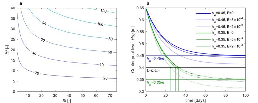
The time scale tL is defined by Equation (9) through non-dimensional discharge Q∗ (R∗ , Bi).
4.2.simulations
For Water Level assuming
Dynamics aand the Rolethaw-layer
constant of Evapotranspiration
thickness L, we likewise assumed that the water level
in theThe trough
timehwscale
remainsisapproximately constant(9)during
defined by Equation thenon-dimensional
through time period of interest. Figure∗3a
discharge ( indicates
∗
, ). For
that discharge increases linearly with the anisotropy-adjusted aspect ratio, R ∗ , for practically any value
simulations assuming a constant thaw-layer thickness L, we likewise assumed that the water level in
of Bi,trough
the the hydraulic conductance
hw remains of the constant
approximately polygon drainage interface.
during the Thisof
time period general graph
interest. can3a
Figure beindicates
utilized
to evaluate
that of the
discharge polygonlinearly
increases drainagewith
dynamics, indicating that discharge
the anisotropy-adjusted is linearly
aspect ratio, ∗ dependent on the
, for practically any
anisotropy-adjusted aspect ratio and is only dependent on the drainage interface
value of , the hydraulic conductance of the polygon drainage interface. This general when its conductance
graph can be
isutilized
significantly low.
to evaluate of the polygon drainage dynamics, indicating that discharge is linearly dependent
on the anisotropy-adjusted aspect ratio and is only dependent on the drainage interface when its
conductance is significantly low.
For illustration, we considered drainage of a typical anisotropic polygon of radius R = 10 m,
thickness L = 0.4 m, and rim–trough interface width l ≈ 0.5 m. Conductive properties were as follows:
Kr = 1 m/day, Kz = 0.2 m/day, and k = 0.5 m day−1 (i.e., κ = 1.0 day−1). The initial center pool level was
H(0) = 0.65 m (i.e., 0.25 m above the ground surface) and the water level in the trough was hw = 0.45
m. These parameters yielded dimensionless values R* = 16.8 and Bi = 0.89. The characteristic time of
this problem was = 18 days. (Sensitivity of results to κ is moderate at these values, as discussed in
Appendix B).
Published experimental data on evapotranspiration E in Siberia [4] and Alaska [7] using various
field methods indicate typical values on the order of 10−3 m day−1. Therefore, we used E = 0.5 ⋅ 10 m
day−1 and E = 2 ⋅ 10 m day−1 to explore the effect on tdrain values.
In Figure 3b, we show the dynamics of the pool water level following Equation (27). Here, water
in the polygon center remains ponded indefinitely (Figure 3b), at the evaporation rates that we
considered, because > L = 0.4 m according to Equation (29).
Figure 3. Drainage dynamics through the polygon: (a) dimensionless function Q∗ (R∗ , Bi∗ ), (b) example
The situation changes if the water level in the trough is at lower elevation than in the polygon
of center pool depth dynamics for specific parameter values with characteristic time scale tL = 18 days
center,
ande.g., if hwevaporation
different = 0.35 m. Equation
rates and (27)
watershows
levels that
in thethe pool Continuous
trough. will drain entirely at actual
lines show any evaporation
water
rate level 0, 0.5 ⋅ in
(E =dynamics 10the ,pool 2 ⋅ 10
andbefore m day −1). Corresponding drainage times, calculated from
complete draining; dashed lines are auxiliary and are mathematical,
non-physical parts of the solution after drainage is complete. Times of draining tdrain are indicated by
stem plots on the time axis.Water 2020, 12, x FOR PEER REVIEW 10 of 14
Equation (30) are tdrain = 33, 30, and 25 days, and are similar to typical conditions observed in the
Arctic, either at the start of the summer or following a large precipitation event in mid-summer [5,8].
Water 2020, 12, 3376 10 of 14
For illustration, we considered drainage of a typical anisotropic polygon of radius R = 10 m,
thickness L = 0.4 m, and rim–trough interface width l ≈ 0.5 m. Conductive properties were as follows:
Kr = 1 m/day, Kz = 0.2 m/day, and k = 0.5 m day−1 (i.e., κ = 1.0 day−1 ). The initial center pool level was
H(0) = 0.65 m (i.e., 0.25 m above the ground surface) and the water level in the trough was hw = 0.45 m.
These parameters yielded dimensionless values R* = 16.8 and Bi = 0.89. The characteristic time of
this problem was tL = 18 days. (Sensitivity of results to κ is moderate at these values, as discussed in
Appendix B).
Published experimental data on evapotranspiration E in Siberia [4] and Alaska [7] using various
field methods indicate typical values on the order of 10−3 m day−1 . Therefore, we used E = 0.5·10−3 m
day−1 and E = 2·10−3 m day−1 to explore the effect on tdrain values.
In Figure 3b, we show the dynamics of the pool water level following Equation (27). Here, water in
the polygon center remains ponded indefinitely (Figure 3b), at the evaporation rates that we considered,
Figure 3. Drainage dynamics through the polygon: (a) dimensionless function ∗ ( ∗ , ∗ ) , (b)
because Hmin > L = 0.4 m according to Equation (29).
example of center pool depth dynamics for specific parameter values with characteristic time scale
The situation changes if the water level in the trough is at lower elevation than in the polygon
= 18 days and different evaporation rates and water levels in the trough. Continuous lines show
center, e.g., if hw = 0.35 m. Equation (27) shows that the pool will drain entirely at any evaporation rate
actual water level dynamics in the pool before complete draining; dashed lines are auxiliary and are
(E = 0, 0.5·10−3 , and 2·10−3 m day−1 ). Corresponding drainage times, calculated from Equation (30) are
mathematical, non-physical parts of the solution after drainage is complete. Times of draining tdrain are
tdrain = 33, 30, and 25 days, and are similar to typical conditions observed in the Arctic, either at the
indicated by stem plots on the time axis.
start of the summer or following a large precipitation event in mid-summer [5,8].
4.3. Calibration of Center Pond Drainage Scenario with Dynamic Thaw-Layer Thickness at Utqiagvik
4.3. Calibration of Center Pond Drainage Scenario with Dynamic Thaw-Layer Thickness at Utqiagvik
Figure 4 presents the results of our calibration of the model against head data from the center
Figure 4 presents the results of our calibration of the model against head data from the center pool
pool in early summer at an inundated low-centered polygon near Utqiagvik, Alaska [5]. The
in early summer at an inundated low-centered polygon near Utqiagvik, Alaska [5]. The simulation
simulation considered piecewise-linear gradual changes to the thickness of the thawed layer beneath
considered piecewise-linear gradual changes to the thickness of the thawed layer beneath the polygon
the polygon center and observations of dynamic water level in the trough pool, as described in
center and observations of dynamic water level in the trough pool, as described in Sections 3.3.5
Sections 3.3.5 and 3.5.2. The final calibration demonstrates a very close match between observed and
and 3.5.2. The final calibration demonstrates a very close match between observed and simulated head
simulated head in the center pool, with a root mean squared error of ~0.006 m. Likewise, the
in the center pool, with a root mean squared error of ~0.006 m. Likewise, the calibrated parameters Kr ,
calibrated parameters Kr, Kz, and κ fit squarely within the ranges defined in Section 3.5.1, with an
Kz , and κ fit squarely within the ranges defined in Section 3.5.1, with an anisotropy ratio Kr /Kz of ~7.6.
anisotropy ratio Kr/Kz of ~7.6. The close match between observed and simulated head and the
The close match between observed and simulated head and the reasonable calibration of hydraulic
reasonable calibration of hydraulic parameters affirms the physical realism of our model in a scenario
parameters affirms the physical realism of our model in a scenario characterized by rapid changes in
characterized by rapid changes in thaw-layer thickness and trough pool water level. A video
thaw-layer thickness and trough pool water level. A video illustrating these results is also available
illustrating these results is also available online in the Supplementary Material.
online in the Supplementary Material.
Figure 4. Observed and simulated center pool water level, from a piecewise-linear simulation of early
summer drainage at a low-centered polygon near Utqiagvik, Alaska, accounting for temporal variability
in thaw-layer thickness beneath the polygon center and water level in the trough pool. A video of this
simulation is available online in the Supplementary Material.Water 2020, 12, 3376 11 of 14
5. Conclusions
We developed a hydrodynamic model of inundated low-centered polygon drainage coupled
with the center pool water balance and obtained an analytical solution. For conditions typically
observed in polygonal tundra, a very strong edge effect was found; only a small fraction of the polygon
located near the edges is flushed by the water drained from center pool storage. Confidence in the
model is bolstered by the fact that simulated characteristic drainage time estimates are consistent with
published observations, and the model accurately simulates the early summer disappearance of the
center pond in a low-centered polygon when solved in a piecewise-linear fashion that accounts for
dynamic thaw-layer thickness and water level in the trough pool. Some of the key insights derived
from the model are:
1. Polygons are flushed most intensively at the edges for practically all existing physical and
geometric parameters. The streamline patterns in this zone change little when the aspect ratio
(radius-to-thickness of active layer) exceeds a value of three.
2. Anisotropy in hydraulic conductivity (horizontal-to-vertical hydraulic conductivity ratio) has a
secondary influence on the intensity of flushing. Increases of anisotropy values counteract the
effects of increased geometrical aspect ratio increases and vice versa (as discussed in Appendix B).
3. Hydraulic resistance of the drainage interface between the polygon and trough also has some
limited, but not overriding influence within the typical range of Arctic tundra conditions.
4. Drainage time scales are consistent with observed duration of the center pool drainage within
low-centered polygons. The parameter tL can be used to characterize drainage times from an
inundated polygon center.
Supplementary Materials: The following are available online at http://www.mdpi.com/2073-4441/12/12/3376/
s1, File S1: Code for model execution, File S2: Video of simulated and observed center pond drainage at
Utqiagvik, Alaska.
Author Contributions: V.A.Z. and D.R.H. conceived the concept for the study. V.A.Z. developed the analytical
model, with context for the hydrological problem provided by D.R.H. and C.J.A., V.A.Z. wrote the original draft
of the manuscript; edits and revisions were contributed by all authors. C.J.A. created figures to visualize the
conceptual model and results. E.E.J. performed the calibration of the GIPL heat-flow model to 2013–2014 BEO,
Site A polygon soil temperature measurements and provided simulated 2012 thaw depths. All authors have read
and agreed to the published version of the manuscript.
Funding: The Next Generation Ecosystem Experiments Arctic (NGEE-Arctic) project (DOE ERKP757), funded by
the Office of Biological and Environmental Research within the U.S. Department of Energy’s Office of Science
provided funding to D.R.H., C.J.A., and E.E.J. for this research.
Acknowledgments: We acknowledge discussions with K. Cole, UNL and thank him for providing a script to
calculate eigenvalues.
Conflicts of Interest: The authors declare no conflict of interest.
Appendix A. Derivation of the Head Distribution and Stokes Stream Function
Using separation of variables for the boundary value problem in Equations (12)–(16) (e.g., [23]),
one obtains:
X∞ cosh(λn z)
h∗ (r∗ , z∗ ) = Bn J0 (λn r∗ ), n = 1, 2, . . . (A1)
n=1 cosh(λn )
where λn , n = 1, 2, . . . are roots of the equation:
λn J1 (λn R∗ ) = Bi·J0 (λn R∗ ), n = 1, 2, . . . (A2)J 0 () and J1() are Bessel functions of the first kind, and coefficients are as follows:
∗
∗ ∗ ∗
( )
= (A3)
∗ 2 ∗) ∗ ∗
(
0
Water 2020, 12, 3376 12 of 14
Estimation of Bn uses identities:
J0 (•) and J1 (•) are Bessel functions of the first kind, and coefficients Bn are as follows:
( ) = ( ), = 1, ( ) = [ ( ) + ( )] (A4)
R R∗
0
J0 (λn r )r dr
∗ ∗ ∗
(See [24], Equations (11.3.20) and =
Bn (11.3.34)) (A3)
R R∗ 2 their special cases:
and
0
J (λn r∗ )r∗ dr∗
∗ 0 ∗ ∗
∗ ∗ ∗
( )
( ) =
Estimation of Bn uses identities: (A5)
∗ ∗
2 ∗ ∗ ∗ 2 ∗ 2
Z z ( ) = Z z ( ) + z(2 h ∗ )
ν 0 ν 2 0
tJ0 (t) dt = 1 J0 2 (z) + J1 2 (z)
i
2
t Jν−1 (t) dt = z Jν (z), ν = 1, (A4)
0 0 2
These identities fully determine coefficients Bn, resulting in Equation (18).
(See [24], Equations (11.3.20) and (11.3.34)) and their special cases:
Appendix B. Role of Hydraulic Resistance R R∗ of the Polygon-trough
R∗ J1 (λn R∗ ) Interface and Anisotropy
0
J0 (λn r∗ )r∗ dr∗ = λn
The parameter BiRaccounts for hydraulic ∗2resistance of the interface between the polygon(A5) and
" #
R∗ 2 2 2
trough (see Equation (7)). J
0 High
(λvalues
∗ ∗
n r )r dr
∗ R
= 2 that
indicate J the (λnhead
R ) +inJ the(λ
∗ ∗
nR )
polygon at the periphery of the
0 0 1
polygon center is near-equal to the head inside the trough. To estimate the effect of this parameter,
These A1,
in Figure identities fully determine
we display streamlines coefficients
near the rim Bn , resulting
of a polygon in Equation (18).
with dimensionless radius ∗ = 10,
∗
within range of radii between 8.5 and 10 (radii between 0 and 8.5 are omitted). Selected values of
Appendix B. Role
(0.01, 1.0, and of
10)Hydraulic Resistance
reflect limited of the Polygon-trough
data available for polygonal soils. Interface and Anisotropy
A comparison
The parameter Bi ofaccounts
streamlinesfor indicates
hydraulicthat the ten-fold
resistance of theincrease
interfaceinbetweenfromthe
1 to 10 has and
polygon more
effect (see
trough thanEquation
the hundred-fold
(7)). Highincrease in Bi from
values indicate that0.01
thetohead
1. Ainreduction in hydraulic
the polygon resistance
at the periphery also
of the
leads to vertical and radial “shrinking” of the streamlines for = 10.
polygon center is near-equal to the head inside the trough. To estimate the effect of this parameter, This phenomenon can be
ininterpreted
Figure A1,as wefollows:
displayastreamlines
better hydraulicnear theconnection
rim of aintensifies
polygon with flushing near the top
dimensionless R =outer
and the
radius ∗ 10,
edges of the active ∗layer in the polygon center. Although the effect is
within range of radii r between 8.5 and 10 (radii between 0 and 8.5 are omitted). Selected values of Bi modest, this comparison
contextualizes
(0.01, 1.0, and 10)the importance
reflect limited of accurately
data availabledefining hydraulic
for polygonal soils.properties in the polygon rim.
Figure A1. Three sets of streamlines corresponding to values of Bi = 0.01, 1.0, and 10. Each stream tube
carries 10% of the flux, so the area (volume) above the lower streamline in each set contains 90% of the
water flux.
A comparison of streamlines indicates that the ten-fold increase in Bi from 1 to 10 has more effect
than the hundred-fold increase in Bi from 0.01 to 1. A reduction in hydraulic resistance also leads to
vertical and radial “shrinking” of the streamlines for Bi = 10. This phenomenon can be interpreted
as follows: a better hydraulic connection intensifies flushing near the top and the outer edges of theWater 2020, 12, 3376 13 of 14
active layer in the polygon center. Although the effect is modest, this comparison contextualizes the
importance of accurately defining hydraulic properties in the polygon rim.
The effect of anisotropy in hydraulic conductivity Kr /Kz is to alter both the parameters R* and
Bi, as indicated in Equation (7). However, a somewhat limited effect of Bi on the kinematic structure
of flow in the polygon generally indicates that anisotropy has moderate influence on the edge effect.
For example, Kr /Kz = 4 would reduce the value of R* by a factor of two, which would be equivalent
to a reduction in R* from 20 to 10 in Figure 2 in the main text. This indicates that an increase in the
anisotropy can redistribute the flux over the polygon, thereby reducing the edge effect.
References
1. Jorgenson, M.T.; Shur, Y.L.; Pullman, E.R. Abrupt increase in permafrost degradation in Arctic Alaska.
Geophys. Res. Lett. 2006, 33, L024960. [CrossRef]
2. Liljedahl, A.; Boike, J.; Daanen, R.; Fedorov, A.N.; Frost, G.V.; Grosse, G.; Hinzman, L.D.; Iijma, Y.;
Jorgenson, J.C.; Matveyeva, N.; et al. Pan-Arctic ice-wedge degradation in warming permafrost and its
influence on tundra hydrology. Nat. Geosci. 2016, 9, 312–318. [CrossRef]
3. Farquharson, L.M.; Romanovsky, V.E.; Cable, W.L.; Walker, D.A.; Kokelj, S.V.; Nicolsky, D. Climate change
drives widespread and rapid thermokarst development in very cold permafrost in the Canadian High Arctic.
Geophys. Res. Lett. 2019, 46, 6681–6689. [CrossRef]
4. Helbig, M.; Boike, J.; Langer, M.; Schreiber, P.; Runkle, B.R.; Kutzbach, L. Spatial and seasonal variability of
polygonal tundra water balance: Lena River Delta, northern Siberia (Russia). Hydrogeol. J. 2013, 21, 133–147.
[CrossRef]
5. Liljedahl, A.K.; Wilson, C.J. Ground Water Levels for NGEE Areas A, B, C, and D, Barrow, Alaska, 2012–2014;
Next Generation Ecosystems Arctic Data Collection; Oak Ridge National Laboratory, U.S. Department of
Energy: Oak Ridge, TN, USA, 2016. [CrossRef]
6. Koch, J.C.; Gurney, K.; Wipfli, M.S. Morphology-dependent water budgets and nutrient fluxes in Arctic thaw
ponds. Permafr. Periglac. Process. 2014, 25, 79–93. [CrossRef]
7. Koch, J.C.; Jorgenson, M.T.; Wickland, K.P.; Kanevskiy, M.; Striegl, R. Ice wedge degradation and stabilization
impact water budgets and nutrient cycling in Arctic trough ponds. J. Geophys. Res. Biogeosci. 2018,
123, 2604–2616. [CrossRef]
8. Wales, N.A.; Gomez-Velez, J.D.; Newman, B.D.; Wilson, C.J.; Dafflon, B.; Kneafsey, T.J.; Wullschleger, S.D.
Understanding the relative importance of vertical and horizontal flow in ice-wedge polygons. Hydrol. Earth
Syst. Sci. 2020, 24, 1109–1129. [CrossRef]
9. Cory, R.M.; Ward, C.P.; Crump, B.C.; Kling, G.W. Sunlight controls water column processing of carbon in
arctic fresh waters. Science 2014, 345, 925–928. [CrossRef] [PubMed]
10. Jan, A.; Coon, E.T.; Painter, S.L.; Garimella, R.; Moulton, J.D. An intermediate-scale model for thermal
hydrology in low-relief permafrost-affected landscapes. Comput. Geosci. 2018, 22, 163–177. [CrossRef]
11. Aas, K.S.; Martin, L.; Nitzbon, J.; Langer, M.; Boike, J.; Lee, H.; Berntsen, T.K.; Westermann, S. Thaw processes
in ice-rich permafrost landscapes represented with laterally coupled tiles in a land surface model. Cryosphere
2019, 13, 591–609. [CrossRef]
12. Nitzbon, J.; Langer, M.; Westermann, S.; Martin, L.; Aas, K.S.; Boike, J. Pathways of ice-wedge degradation in
polygonal tundra under different hydrological conditions. Cryosphere 2019, 13, 1089–1123. [CrossRef]
13. Nitzbon, J.; Westermann, S.; Langer, M.; Martin, L.C.; Strauss, J.; Laboor, S.; Boike, J. Fast response of cold
ice-rich permafrost in northeast Siberia to a warming climate. Nat. Commun. 2020, 11, 2201. [CrossRef]
14. Dobinksi, W. Permafrost active layer. Earth Sci. Rev. 2020, 208, 103301.
15. Abolt, C.J.; Young, M.H. High-resolution mapping of spatial heterogeneity in ice wedge polygon
geomorphology near Prudhoe Bay, Alaska. Sci. Data 2020, 7, 87. [CrossRef] [PubMed]
16. Quinton, W.L.; Hayashi, M.; Carey, S.K. Peat hydraulic conductivity in cold regions and its relation to pore
size and geometry. Hydrol. Process. 2008, 22, 2829–2837. [CrossRef]
17. Abolt, C.J.; Young, M.H.; Caldwell, T.G. Numerical modelling of ice-wedge polygon geomorphic transition.
Permafr. Periglac. Process. 2017, 28, 347–355. [CrossRef]
18. Beckwith, C.W.; Baird, A.; Heathwaite, A.L. Anisotropy and depth-related heterogeneity of hydraulic
conductivity in a bog peat. I: Laboratory measurements. Hydrol. Process. 2003, 17, 89–101. [CrossRef]Water 2020, 12, 3376 14 of 14
19. Chason, D.B.; Siegel, D.I. Hydraulic conductivity and related physical properties of peat, Lost River Peatland,
Northern Minnesota. Soil Sci. 1986, 142, 91–99. [CrossRef]
20. Ebel, B.A.; Koch, J.C.; Walvoord, M.A. Soil physical, hydraulic, and thermal properties in interior Alaska,
USA: Implications for hydrologic response to thawing permafrost conditions. Water Resour. Res. 2019,
55, 4427–4447. [CrossRef]
21. Rodell, M.; Houser, P.R.; Jambor, U.; Gottschalck, J.; Mitchell, K.; Meng, C.-J.; Arsenault, K.; Cosgrove, B.;
Radakovich, J.; Entin, M.B.J.K.; et al. The Global Land Data Assimilation System. Bull. Am. Meteorol. Soc.
2004, 85, 381–394. [CrossRef]
22. Jafarov, E.E.; Marchenko, S.S.; Romanovsky, V.E. Numerical modeling of permafrost dynamics in Alaska
using a high spatial resolution dataset. Cryosphere 2012, 6, 613–624. [CrossRef]
23. Mackowski, D.W. Conduction Heat Transfer, Notes for MECH 7210. Mechanical Engineering Dept., Auburn
University, 2020. Available online: http://www.eng.auburn.edu/~{}dmckwski/mech7210/condbook.pdf
(accessed on 24 September 2020).
24. Abramowitz, M.; Stegun, I. Handbook of Mathematical Functions: With Formulas, Graphs, and Mathematical
Tables; Dover Publications: Mineola, NY, USA, 1965.
Publisher’s Note: MDPI stays neutral with regard to jurisdictional claims in published maps and institutional
affiliations.
© 2020 by the authors. Licensee MDPI, Basel, Switzerland. This article is an open access
article distributed under the terms and conditions of the Creative Commons Attribution
(CC BY) license (http://creativecommons.org/licenses/by/4.0/).You can also read