Positional Value in Soccer: Expected League Points Added above Replacement - arXiv
←
→
Page content transcription
If your browser does not render page correctly, please read the page content below
Positional Value in Soccer: Expected League Points Added above
                                                                                Replacement
                                                                         Konstantinos Pelechrinis∗ and Wayne Winston†

                                           Abstract. Soccer is undeniably the most popular sport world-wide, but at the same time it is one of the least
                                                     quantified. To date there is not a way to explicitly quantify the contribution of every player on
                                                     the field to his team chances of winning. Successful sports metrics, such as the (adjusted) +/- that
                                                     allows for division of credit among a basketball team’s players, fail to work in soccer due to severe
                                                     co-linearities (i.e., the same players being on the field for the majority of the time). In this work,
                                                     we develop a framework that can estimate the expected contribution of a soccer player to his team’s
                                                     winning chances. In particular, using data from (i) approximately 20,000 games from 11 European
arXiv:1807.07536v3 [stat.AP] 20 Aug 2018

                                                     leagues for 8 seasons, as well as, (ii) player ratings from FIFA, we estimate through a Skellam
                                                     regression model the importance of every line in winning a soccer game. We consequently translate
                                                     the model to expected league points added (per game) above a replacement player eLPAR. This
                                                     model can be used as a guide for player transfer decisions, as well as, for transfer fees and contract
                                                     negotiations among other applications. To showcase the applicability of eLPAR we use market value
                                                     data for approximately 10,000 players and we identify evidence that currently the market under-
                                                     values defensive line players relative to goalkeepers. Finally, we discuss how our framework can be
                                                     significantly enhanced using player tracking data, but also, how it can be used to obtain positional
                                                     (and consequently player) value for American football, which is another sports where achieving
                                                     division of credit has been proven to be hard to date.

                                               1. Introduction. Soccer is undoubtedly the king of sports, with approximately 4 billion
                                           global following [28]. However, despite this huge global interest it still lags behind with respect
                                           to advanced quantitative analysis and metrics capturing teams’ and players’ performance as
                                           compared to other sports with much smaller fan base (e.g., baseball, basketball). Traditionally
                                           sports metrics quantify on-ball events. However, soccer epitomizes the notion of team sports
                                           through a game of space and off-ball movement. In soccer every player has possession of the
                                           ball an average of only 3 minutes [8], and hence, metrics that quantify on-ball events will fail
                                           to capture a player’s influence on the game.
                                               Expected goals (xG) [18, 7] is probably the most prominent, advanced metric used in
                                           soccer today. xG takes into account the context of a shot (e.g., location, number of defenders
                                           in the vicinity etc.) and provides us with the probability of a shot leading to a goal. xG allows
                                           us to statistically evaluate players. For example, if a player is over-performing his expected
                                           goals, it suggests that he is either lucky or an above-average finisher. If this over-performance
                                           persists year-after-year then the latter will be a very plausible hypothesis. Nevertheless, while
                                           expected goals represent a straightforward concept and has been already used by mainstream
                                           soccer broadcast media, its application on evaluating players is still limited to a specific aspect
                                           of the game (i.e., shot taking) and only to players that actually take shots (and also potentially
                                           goalkeepers). A more inclusive version of xG, is the Expected Goal Chains (xGC) [21]. xGC
                                           considers all passing sequences that lead to a shot and credits each player involved with the
                                           expected goal value for the shot. Of course, not all passes are created equally [20] and hence,
                                             ∗
                                                  School of Computing and Information, University of Pittsburgh (kpele@pitt.edu)
                                              †
                                                  Kelly School of Business, Indiana University (wayne@indiana.edu)
                                                                                                    1

                                                                          This manuscript is for review purposes only.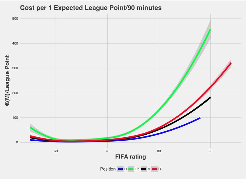
2                                                        KONSTANTINOS PELECHRINIS, WAYNE WINSTON

xGC can over/under estimate the contribution of a pass to the final shot.
     The last few years player tracking technology has started penetrating the soccer industry.
During the last world cup in Russia, teams obtained player tracking data in real time [6]!
The availability of fine-grained spatio-temporal data have allowed researchers to start looking
into more detailed ways to evaluate soccer players through their movement in space. For
example, Hoang et al. [16, 15] developed a deep imitation learning framework for identifying
the optimal locations - i.e., the ones that minimize the probability of conceding a goal - of the
defenders in any given situation based on the locations of the attackers (and the other defensive
players). Fernandez and Bornn [8] also analyzed player tracking data and developed a metric
quantifying the contribution of players in space creation as well as, this space’s value, while a
nice overview of the current status of advanced spatio-temporal soccer analytics is provided
by Bornn et al. [4]. Player tracking data will undoubtedly provide managers, coaches and
players with information that previously was considered to be intangible, and revolutionize
soccer analytics. However, to date all of the efforts are focused on specific aspects of the
game. While in the future we anticipate that a manager will be able to holistically evaluate
the contribution of a player during a game over a number of dimensions (e.g., space generation,
space coverage, expected goals etc.), currently this is not the case - not to mention that player
tracking technology is still slow in widespread adoption. Therefore, it has been hard to develop
soccer metrics similar to Win Shares and/or Wins Above Replacement Player that exist for
other sports (e.g., baseball, basketball etc.) [11, 25]. These - all-inclusive - metrics translate
on field performance to what managers, coaches, players and casual fans can understand,
relate to and care about, i.e., wins.
     Our study aims at filling exactly this gap in the existing literature discussed above. The
first step towards this is quantifying the positional values in soccer. For instance, how much
more important are the middle-fielders compared to the goalkeeper when it comes to winning
a game? In order to achieve this we use data from games from 11 European leagues as well as
FIFA ratings for the players that played in these games. These ratings have been shown to be
able to drive real-world soccer analytics studies [5] and they are easy to obtain1 . Using these
ratings we model the final goal differential of a game through a Skellam regression that allows
us to estimate the impact of 1 unit of increase of the FIFA rating for a specific position on
the probability of winning the game. As we will elaborate on later, to avoid any data sparsity
problems (e.g., very few team play with a sweeper today), we group positions in the four
team lines (attack, middle-field, defense and goalkeeping) and use as our model’s independent
variables the difference on the average rating of the corresponding lines. Using this model
we can then estimate the expected league points added above replacement (eLPAR) for
every player. The emphasis is put on the fact that this is the expected points added from
a player, since it is based on a fairly static, usually pre-season, player rating, and hence,
does not capture the exact performance of a player in the games he played, even though the
FIFA ratings change a few times over the course of a season based on the overall player’s
performance. However, when we describe our model in detail it should become evident that
if these data (i.e., game-level player ratings) are available the exact same framework can be
used to evaluate the actual league points added above replacement from every player.

    1
        Data and code are available:https://github.com/kpelechrinis/eLPAR-soccer.

                               This manuscript is for review purposes only.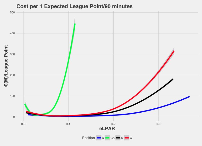
POSITIONAL VALUE IN SOCCER: EXPECTED LEAGUE POINTS ADDED ABOVE REPLACEMENT                                 3

    The contribution of our work is twofold:
     1. We develop a pre-game win probability model for soccer that is accurate and well-
        calibrated. More importantly it is based on the starting lineups of the two teams and
        hence, it can account for personnel changes between games.
     2. We develop the expected league points added above replacement (eLPAR) metric that
        can be used to identify positional values in soccer and facilitate quantitative (mone-
        tary) player valuation in a holistic way.
    Section 2 describes the data we used as well as the regression model we developed for
the score differential. Section 3 further details the development of our expected league points
added above replacement using the Skellam regression model. In this section we also discuss
the implications for the players’ transfer market. Finally, Section 4 discusses the scope and
limitations of our current study, as well as, future directions for research.
    2. Data and Methods. In this section we will present the data that we used for our
analysis, existing modeling approaches for for the goal differential in a soccer game, as well
as, the Skellam regression model we used.
     2.1. Soccer Dataset. In our study we make use of the Kaggle European Soccer Database
[1]. This dataset includes all the games (21,374 in total) from 11 European leagues2 between
the seasons 2008-09 and 2015-16. For every game, information about the final result as well
as the starting lineups are provided. There is also temporal information on the corresponding
players’ ratings for the period covered by the data. A player’s p rating takes values between
0 and 100 and includes an overall rating rp , as well as sub-ratings for different skills (e.g.,
tackling, dribbling etc.). There are 11,060 players in totals and an average of 2 rating readings
per season for every player. One of the information that we need for our analysis and is not
present in the original dataset, is the players’ position and his market value. We obtained this
information through FIFA’s rating website (www.sofifa.com) for all the players in our dataset.
     The goals scored in a soccer game have traditionally been described through a Poisson
distribution [17, 12], while a negative binomial distribution has also been proposed to account
for possible over-dispersion in the data [19, 9]. However, the over-dispersion, whenever ob-
served is fairly small and from a practical perspective does not justify the use of the negative
binomial for modeling purposes considering the trade-off between complexity of estimating
the models and improvement in accuracy [12]. In our data, we examined the presence of over-
dispersion through the Pearson chi-squared dispersion test. We performed the test separately
for the goal scored from home and away teams and in both cases the dispersion statistic is
very close to 1 (1.01 and 1.1 respectively), which allows us to conclude that a Poisson model
fits better for our data. Figure 1 depicts the two distributions for the goals scored per game
for the home and away teams in our dataset.
     Another important modeling question is the dependency between the two Poisson pro-
cesses that capture the scoring for the two competing teams. In general, the empirical
data exhibit a small correlation (usually with an absolute value for the correlation coeffi-
cient less than 0.05) between the goals scored by the two competing teams and the use of

   2
    English Premier League, Bundesliga, Serie A, Scotish Premier League, La Liga, Swiss Super League, Jupiler
League, Ligue 1, Eredivisie, Liga Zon Sagres, Ekstraklasa.

                            This manuscript is for review purposes only.
4 KONSTANTINOS PELECHRINIS, WAYNE WINSTON
Figure 1. The empirical distribution of the number of goals scored per game from the home (left) and way
(right) teams. The data can be fitted by a Poisson with means λ = 1.56 and λ = 1.18 respectively.
Bivariate Poisson models has been proposed to deal with this correlation [13]. Simple put,
(X, Y ) ∼ BP (λ1 , λ2 , λ3 ), where:
min(x,y)
x λy2 λ3 k
−(λ1 +λ2 +λ3 ) λ1 x y
X
(2.1) P (X = x, Y = y) = e k!
x! y! k k λ1 λ2
k=0
The parameter λ3 captures the covariance between the two marginal Poisson distributions for
X and Y , i.e., λ3 = Cov(X, Y ). In our data, the correlation between the number of goals
scored from the home and away team is also small and equal to -0.06. While this correlation is
small, Karlis and Ntzoufras [13] showed that it can impact the estimation of the probability of
a draw. However, a major drawback of the Bivariate Poisson model is that it can only model
data with positive correlations [14]. Given that in our dataset the correlation is negative, and
hence, a Bivariate Poisson model cannot be used, an alternative approach is to directly model
the difference between the two Poisson processes that describe the goals scored for the two
competing teams. With Z, X and Y being the random variables describing the final score
differential, the goals scored from the home team and the goals scored from the away team
respectively, we clearly have Z = X − Y . With (X, Y ) ∼ BP (λ1 , λ2 , λ3 ), Z has the following
probability mass function [22]:
z/2
λ1 +λ2 λ1 p
(2.2) P (z) = e · · Iz (2 λ1 λ2 )
λ2
where Ir (x) is the modified Bessel function. Equation (2.2) describes a Skellam distribution
and clearly shows that the distribution of Z does not depend on the correlation between the two
Poisson distributions X and Y . In fact, Equation (2.2) is exactly the same as the distribution
of the difference of two independent Poisson variates [22]. Therefore, we can directly model the
This manuscript is for review purposes only.POSITIONAL VALUE IN SOCCER: EXPECTED LEAGUE POINTS ADDED ABOVE REPLACEMENT 5
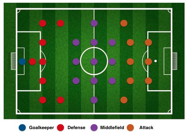
Figure 2. For our analysis we grouped the various player positions to four distinct groups, namely, goal-
keeping, attack, middlefielders and defense.
goal differential without having to explicitly model the covariance. Of course, the drawback
of this approach is that the derived model is not able to provide estimates on the actual
game score, but rather only on the score differential. Nevertheless, in our study we are not
interested in the actual score but rather in the win/lose/draw probability. Hence, this does
not pose any limitations for our work.
2.2. Skellam Regression Model. Our objective is to quantify the value of different posi-
tions in soccer. This problem translates to identifying how an one-unit increase in the rating of
a player’s position impacts the probability of his team winning. For instance, if we substitute
our current striker who has a FIFA rating of 79, with a new striker with a FIFA rating of 80,
how do our chances of winning alter? Once we have this information we can obtain for every
player an expected league points added per game over a reference, i.e., replacement, player
(Section 3.1). This can then be used to obtain a more objective market value for players based
on their position and rating (Section 3.2).
In order to achieve our goal we model the goal differential Z of a game using as our
independent variables the player/position ratings of the two teams that compete. Hence, our
model’s dependent variable is the goal differential (home - away) of game i, zi , while our
independent variables are the positional rating differences of the two teams, xi,π = rp(h,π,i) −
rp(a,π,i) , ∀π ∈ Π, where rp(h,π,i) (rp(a,π,i) ) is the rating of the home (away) team player that
covers position π during game i and Π is the set of all soccer positions. One of the challenges
with this setting is the fact that different teams will use different formations and hence, it can
be very often the case that while one team might have 2 center backs and 2 wing backs, the
other team might have 3 center backs only in its defensive line. This will lead to a situation
where the independent variables xi,π might not be well-defined. While this could potentially
be solved by knowing the exact formation of a team (we will elaborate on this later), this
This manuscript is for review purposes only.6 KONSTANTINOS PELECHRINIS, WAYNE WINSTON
is unfortunately a piece of information missing from our data. Nevertheless, even this could
create data sparsity problems (e.g., formation/player combinations that do not appear often).
Hence, we merge positions to four groups, namely, attacking line, middle-fielders, defensive
line and goalkeeping. Figure 2 depicts the grouping of the positions we used to the four lines
Λ = {λD , λM , λA , λGK }. Note that this grouping in the four lines has been used in the past
when analyzing soccer players as well [10]. The independent variables of our model are then
the differences in the average rating of the corresponding lines. The interpretation of the
model slightly changes now, since the independent variable captures the rating of the whole
line as compared to a single position/player. Under this setting we fit a Skellam regression
for Z through maximum likelihood estimation. In particular:
Model 2.1: Final Goal Differential
We model the goal differential Zi of game i using the following four co-variates:
• The difference between the average player rating of the defensive line of the two
teams xD
• The difference between the average player rating of the middle-fielders of the
two teams xM
• The difference between the average player rating of the attacking line of the two
teams xA
• The difference between the goalkeeper’s rating of the two teams xGK
The random variable Z follows a Skellam distribution, where its parameters
depend on the model’s covariates x = (xD , xM , xA , xGK ):
(2.3) Z ∼ Skellam(λ1 , λ2 )
(2.4) log(λ1 ) = bT1 · x
(2.5) log(λ2 ) = bT2 · x
Table 1 shows the regression coefficients. It is interesting to note that the coefficients
for the two parameters are fairly symmetric. λ1 and λ2 can be thought of as the mean of
the Poisson distributions describing the home and visiting team respectively and hence, a
positive relationship between an independent variable and the score differential for one team
corresponds - to an equally strong - negative relationship between the same variable and the
score differential. An additional thing to note is that an increase on the average rating of
any line of a team contributes positively to the team’s chances of winning (as one might have
expected).
Before using the model for estimating the expected league points added above replace-
ment for each player, we examine how good the model is in terms of actually predicting the
score differential and the win/draw/lose probabilities. We use an 80-20 split for training and
testing of the model. We begin our evaluation by calculating the difference between the goal
differential predicted by our model and the actual goal differential of the game [23]. Figure
3 (top) presents the distribution of this difference and as we can see it is centered around 0,
while the standard deviation is equal to 1.6 goals. Furthermore, a chi-squared test cannot
This manuscript is for review purposes only.POSITIONAL VALUE IN SOCCER: EXPECTED LEAGUE POINTS ADDED ABOVE REPLACEMENT 7
Variable log(λ1 ) log(λ2 )
Intercept 0.37*** 0.07***
(0.012) (0.015)
xD 0.02*** -0.03***
(0.01) (0.002)
xM 0.02*** -0.015***
(0.01) (0.002)
xA 0.01*** -0.01***
(0.001) (0.001)
xGK 0.001 -0.004**
(0.001) (0.002)
N 21,374 21,374
*** p < 0.01, ** p < 0.05, * p < 0.1
Table 1
Skellam regression coefficients
reject the hypothesis that the distribution is normal with mean equal to 0 and a standard
deviation of 1.6.
However, apart from the score differential prediction error, more important for our pur-
poses is the ability to obtain true win/loss/draw probabilities for the games. As we will see
in Section 3.1 we will use the changes in these probabilities to calculate an expected league
points added for every player based on their position and rating. Hence, we need to evalu-
ate how accurate and well-calibrated these probabilities are. Figure 3 (bottom) presents the
probability calibration curves. Given that we have 3 possible results (i.e., win, loss and draw),
we present three curves from the perspective of the home team, that is, a home team win,
loss or draw. The x-axis presents the predicted probability for each event, while the y-axis is
the observed probability. In particular we quantize the data in bins of 0.05 probability range,
and for all the games within each bin we calculate the fraction of games for which the home
team won/lost/draw, and this is the observed probability. Ideally, we would like to have these
two numbers being equal. Indeed, as we can see for all 3 events the probability output of
our model is very accurate, that is, all lines are practically on top of the y = x line. It is
interesting to note, that our model does not provide a draw probability higher than 30% for
any of the games in the test set, possibly due to the fact that the base rate for draws in the
whole dataset is about 25%.
3. eLPAR and Market Value. We begin by defining the notion of a replacement player
and developing eLPAR. We also show how we can use eLPAR to obtain objective player and
transfer fee (monetary) valuations.
3.1. Replacement Player and Expected League Points Added. The notion of replace-
ment player was popularized by Keith Woolner [27] who developed the Value Over Replace-
ment Player (VORP) metric for baseball. The high level idea is that player talent comes at
This manuscript is for review purposes only.8 KONSTANTINOS PELECHRINIS, WAYNE WINSTON
Figure 3. Our model is able to predict the score differential as well as the win/loss/draw probabilities fairly
accurate.
different levels. For instance, there are superstar players, average players and subpar player
talent. These different levels come in different proportions within the pool of players, with
superstars being a scarcity, while subpar players (what Woolner termed replacement players)
being a commodity. This essentially means that a team needs to spend a lot of money if it
wants to acquire a superstar, while technically a replacement player comes for free. Since a re-
placement player can be thought of as a free player, a good way to evaluate (and consequently
estimate a market value for) a player is to estimate the (expected) contribution in wins, points
etc. that he/she offers above a replacement player. One of the main contributions of Woolner’s
work is to show that average players have value [25]! If we were to use the average player as our
reference for evaluating talent, we would fail to recognize the value of average playing time.
Nevertheless, replacement level, even though it is important for assigning economic value to
a player, it is a less concrete mathematical concept. There are several ways that have been
used to estimate this. For example, one can sort players (of a specific position) in decreasing
order of their contract value and obtain as replacement level the talent at the bottom 20th
percentile [24]. What we use for our study is a rule-of-thumb suggested from Woolner [26].
In particular, the replacement level is set at the 80% of the positional average rating. While
the different approaches might provide slightly different values for a replacement player, they
will not affect the relative importance of the various positions identified by the model. Figure
4 presents the distribution of the player ratings for the different lines for the last season in
our dataset - i.e., 2015-16. The vertical green lines represent the replacement level for every
position/line, i.e., 80% of the average of each distribution. As we can see all replacement
levels are very close to each other and around a rating of 56. So the question now becomes
how are we going to estimate the expected league points added above replacement (eLPAR)
given the model from Section 2.2 and the replacements levels of each line. First let us define
eLPAR more concretely:
This manuscript is for review purposes only.POSITIONAL VALUE IN SOCCER: EXPECTED LEAGUE POINTS ADDED ABOVE REPLACEMENT 9
Figure 4. The replacement level rating (green vertical line) for each one of the positional lines in soccer is
around 56.
Definition 3.1: eLPAR
Consider a game between teams with only replacement players. Player p substitutes
a replacement player in the lineup. eLPARp describes how many league points (win=3
points, draw = 1 point, loss = 0 points) p is expected to add for his team.
Based on the above definition, eLPARp can be calculated by estimating the change in
the win/draw/loss probability after substituting a replacement player with p. However, the
win probability model aforementioned does not consider individual players but rather lines.
Therefore, in order to estimate the expected points to be added by inserting player p in
the lineup we have to consider the formation used by the team. For example, a defender
substituting a replacement player in a 5-3-2 formation will add a different value of expected
points as compared to a formation with only 3 center-backs in the defensive line. Therefore,
in order to estimate eLPARp we need to specify the formation we are referring to. Had the
formation been available in our dataset we could have built a multilevel model, where each
This manuscript is for review purposes only.10 KONSTANTINOS PELECHRINIS, WAYNE WINSTON
combination of position and formation would have had their own coefficients3 . Nevertheless,
since this is not available our model captures the formation-average value of each line. In
particular, eLPARp for player p with rating rp can be calculated as following:
1. Calculate the increase in the average rating of the line λ ∈ Λ where p substituted the
replacement player based on rp , formation φ and the replacement player rating for the
line rreplacement,φ,λ
2. Calculate, using the win probability model above, the change in the win, loss and draw
probability (δPw , δPd and δPl respectively)
3. Calculate eLPARp (φ) as:
(3.1) eLPARp (φ) = 3 · δPw + 1 · δPd
It should be evident that by definition a replacement player has eLPAR = 0 - regardless
of the formation - while if a player has rating better than a replacement, his eLPAR will
be positive. However, the actual value and how it compares to players playing in different
positions will depend on the formation. In Figure 5 we present the expected league points
added per game for players with different ratings (ranging from 50 to 99) and for different
formations. While there are several different formations that a team can use, we chose 4 of
the most often used ones.
One common pattern in all of the formations presented is the fact that for a given player
rating goal keepers provide the smallest expected league points above replacement - which
is in line with other studies/reports for the value of goal keepers in today’s soccer [3]. It
is also evident that depending on the formation the different positions offer different value.
For example, a 4-5-1 system benefits more from an attacker with a rating of 90 as compared
to a defender with the same rating, while in a 3-5-2 formation the opposite is true. It is
also interesting to note that for a 4-4-2 formation, the value added above replacement for
the different positions are very close to each other (the closest compared to the rest of the
formations). This most probably is due to the fact that the 4-4-2 formation is the most
balanced formation in soccer, and hence, all positions contribute equally to the team. To
reiterate this is an expected value added, i.e., it is not based on the actual performance of a
player but rather on static ratings for a player. Given that teams play different formations over
different games (or even during the same game after in-game adjustments), a more detailed
calculation of eLPAR would include the fraction of total playing time spent by each player on
a specific formation. With T being the total number of minutes played by p, and tφ the total
minutes he played in formation φ, we have:
1X
(3.2) eLPARp = tφ · eLPARp (φ)
T
φ
The last row in Figure 5 presents the average eLPAR for each position and player rating
across all the four possessions (assuming equal playing time for all formations). As we can see
3
And in this case we would also be able to analyze better the impact of positions within a line (e.g., value
of RB/LB compared to CB).
This manuscript is for review purposes only.POSITIONAL VALUE IN SOCCER: EXPECTED LEAGUE POINTS ADDED ABOVE REPLACEMENT 11
Figure 5. Expected league points added above replacement for different formations, player ratings and
positions.
for the same player rating, a defender adds more expected league points above replacement,
followed by an attacker with the same rating. A middlefielder with the same rating adds
only slightly less expected league points compared to an attacker of the same rating, while a
goal keeper (with the same rating) adds the least amount of expected league points. A team
manager can use this information to identify more appropriate targets given the team style
play (formations used) and the budget. In the following section we will explore the relation
This manuscript is for review purposes only.12 KONSTANTINOS PELECHRINIS, WAYNE WINSTON
between the market value of a player and his eLPAR.
3.2. Positional Value and Player Market Value. In this section we will explore how
we can utilize eLPAR to identify possible inefficiencies in the player’s transfer market. In
particular, we are interested in examining whether the transfer market overvalues specific
positions based on the eLPAR value they provide. Splitting the players in the four lines
Figure 6 (left) presents the differences between the average market value - that is, the transfer
fee paid from a team to acquire a player under contract - for each position. As we can see, on
average, defenders are the lowest paid players! However, as aforementioned (Figure 5) for a
given player rating, a defensive player provides the maximum eLPAR value.
Nevertheless, what we are really interested in is the monetary value that a team pays
for 1 expected league point above replacement per game for each player. Granted there is a
different supply of players in different positions. For example, only 8.5% of the players are
goal keepers, as compared to approximately 35% of defenders4 , and hence, one might expect
goalkeepers to be paid more than defenders. However, there is also smaller demand for these
positions and hence, we expect these two to cancel out to a fairly great extend, at least to an
extend that does not over-inflate the market values. Hence, we calculate the monetary cost the
players market values imply that teams are willing to pay for 1 expected league point. Figure 6
(middle) presents the cost (in Euros) per 1 expected league point for different positions and as
a function of the eLPAR they provide. An efficient market would have four straight horizontal
lines, one on top of the other, since the value of 1 expected league point should be the same
regardless of where this point is expected from. However, what we observe is that the market
over-values significantly goal keepers (even though on average they are only the 3rd highest
paid line), and this is mainly a result of their low eLPAR (the best goalkeeper in our dataset
provides an eLPAR of just over 0.1 per 90 minutes). Furthermore, teams appear to be willing
to pay a premium for expected league points generated by the offense as compared to points
generated by the defense, and this premium increases with eLPAR. This becomes even more
clear from the right plot in Figure 6, where teams are willing to pay multiples in premium for
1 expected league point coming from a goalkeeper with 88 FIFA rating as compared to the
same contribution coming from a defender with 86 FIFA rating.
Player wages exhibit similar behavior (the ranking correlation between transfer/market
value and a player’s wage is 0.94). Given that there is no salary cap in European soccer,
teams can potentially overpay in general in order to bring in the players they want. Hence,
across-teams comparisons might not be appropriate. However, within team comparison of
contracts among its players is one way to explore whether teams are being rational in terms
of payroll. In particular, we can examine the distribution of their total budget among their
players, and whether this is in line with their positional values. Simply put, this analysis will
provide us with some relative insight on whether teams spend their budget proportional to
the positional and personal on-field value (i.e., FIFA rating) of each player. Let us consider
two specific teams, that is, FC Barcelona and Manchester United. We will use the wages
of the starting 11 players of the two teams (from the 2017-18 season) and considering the
total budget B constant we will redistribute it based on the eLPAR of each player. Table
4
There is another approximately 35% of middlefielders and 21% of attackers.
This manuscript is for review purposes only.POSITIONAL VALUE IN SOCCER: EXPECTED LEAGUE POINTS ADDED ABOVE REPLACEMENT 13
Figure 6. Even though goalkeepers are among the lowest paid players in soccer, they still are overpaid in
terms of expected league points contributions. Defenders are undervalued when it comes to contributions in
winning.
FC Barcelona
Players FIFA Rating Wage (e) eLPAR eLPAR Wage eLPAR eLPAR Wage
(e) (4-4-2) (4-4-2) (e)
M. Stegen 87 185K 0.106 97K 0.106 102K
S. Roberto 82 150K 0.307 283K 0.285 276K
Pique 87 240K 0.359 330.5K 0.333 323K
S. Umtiti 84 175K 0.328 302K 0.304 295K
Jordi Alba 87 185K 0.359 330.5K 0.333 323K
O. Dembele 83 150K 0.268 246.5K 0.272 264K
I. Rakitic 86 275K 0.295 272K 0.301 291K
s. Busquets 87 250K 0.305 280.5K 0.31 300K
Coutinho 87 275K 0.305 280.5K 0.31 300K
L. Messi 94 565K 0.335 308K 0.292 283K
L. Suarez 92 510K 0.319 294K 0.278 269K
Table 2
FC Barcelona wages and eLPAR-based projected wages.
2 presents the starting 11 for Barcelona, their FIFA rating and their wage5 , while Table 3
presents the same information for Manchester United6 . We have also included the formation-
agnostic (i.e., average of the four most frequent formations aforementioned) eLPAR and the
corresponding redistribution of salaries, as well as the same numbers for the default formation
of each team (4-4-2 for Barcelona and 4-3-3 for Manchester United). The way we calculate
the re-distribution is as following:
eLPARp
1. Calculate the fraction fp = of total eLPAR that player p contributes to his
P11 eLPARtotal
team (eLPARtotal = p=1 eLPARp )
2. Calculate the eLPAR-based wage for player p as fp · B
As we can see there are differences in the wages projected when using eLPAR. Both teams
5
www.sofifa.com/team/241
6
www.sofifa.com/team/11
This manuscript is for review purposes only.14 KONSTANTINOS PELECHRINIS, WAYNE WINSTON
Manchester United
Players FIFA Rating Wage (e) eLPAR eLPAR Wage eLPAR eLPAR Wage
(e) (4-3-3) (4-3-3) (e)
De Gea 91 295K 0.118 79K 0.118 82K
A. Valencia 83 130K 0.328 214K 0.295 206.5K
C. Smalling 81 120K 0.298 200K 0.275 193K
V. Lindelof 78 86K 0.265 179K 0.246 172K
A. Young 79 120K 0.276 186K 0.255 179K
N. Matic 85 180K 0.286 193K 0.387 271K
A. Herrera 83 145K 0.268 181K 0.362 254K
P. Pogba 88 250K 0.314 212K 0.424 297K
J. Lingard 81 115K 0.229 155K 0.133 93.5K
R. Lukaku 86 210K 0.27 183K 0.158 111K
A. Sanchez 88 325K 0.287 194K 0.168 118K
Table 3
Manchester United wages and eLPAR-based projected wages.
for example appear to overpay their goalkeepers based on their expected league points above
replacement per 90 minutes. Of course, some players are under-valued, and as we can see
these players are mainly in the defensive line. These results open up interesting questions for
soccer clubs when it comes to budget decisions. Budget is spent for two reasons; (a) to win,
as well as, (b) to maximize the monetary return (after all, sports franchises are businesses).
The premium that clubs are willing to pay an attacker over a defender for the same amount of
league points can be seen as an investment. These players bring fans in the stadium, increase
gate revenue (e.g., through increased ticket prices), bring sponsors, sell club merchandise, etc.
For example, even though attackers are approximately only 20% of the players’ pool, 60% of
the top-selling jerseys in England during 2018 belonged to attackers [2]. Therefore, when we
discuss the money spent from a team for a transfer (or a wage), winning is only one part of
the equation. While teams with large budgets (like Manchester United and Barcelona) might
be able to pay premiums as an investment, other teams in the middle-of-the-pack can achieve
significant savings, without compromising their chances of winning. In fact, clubs with limited
budget can maximize their winning chances, which is an investment as well (winning can bring
in revenues that can then be used to acquire better/more popular players and so on). A club
with a fixed transfer budget B can distribute it in such a way that maximizes the expected
league points bought (even under positional constraints). For instance, with B = 10 millions
and with the need for a center back and a goalkeeper, if we use the average market values for
the two positions we should allocate 55% of the budget (i.e., 5.5 millions) for the goalkeeper
and 45% of the budget for the defender. This will eventually get us about 0.315 expected
league points per 90 minutes (a goalkeeper with a 77.5 FIFA rating and a defender with a
76.5 FIFA rating). However, if we allocate 2 millions for the goalkeeper and 8 millions for the
defender this will get us around 0.34 expected league points (a goalkeeper with 74 FIFA rating
and a defender with 79 FIFA rating), or simply put the team will have bought 1 expected
This manuscript is for review purposes only.POSITIONAL VALUE IN SOCCER: EXPECTED LEAGUE POINTS ADDED ABOVE REPLACEMENT 15
Figure 7. In Premier League 1M Euros in transfer budget is worth 0.44 league points.
league point at a 7.5% discount as compared to the rest of the market.
3.3. Fair Transfer Fees. In the last example above, the transfer fees mentioned are based
on the current market transfer and most probably will still be an overpayment for the talent
acquired. What basically one can achieve with an approach as the one described above is to
optimize the team’s transfers based on the current market values. However, we can use our
model and analysis to also estimate a fair (i.e., considering only a team’s winning chances)
transfer fee for a player. For this we would need to know what 1M Euros is worth in terms of
league points. To do so we will need the total transfer budget of teams and the total number
of league points they obtained. For example, Figure 7 presents the relationship between a
team’s transfer budget and the total points obtained for the 2017-18 Premier League. The
slope of the linear fit is 0.44 (R2 = 0.71), which means that 1M Euros in transfer budget is
worth 0.44 Premier League points. Therefore for a player p with eLPARp , who is expected to
N · eLPARp
play N games, a fair transfer fee is . For example, recently a transfer that was
0.44
discussed a lot was that of goal keeper Danny Ward from Liverpool to Leicester. Based on
Ward’s current rating (70) and his potential upside (78), the transfer fee should be between
4.6 and 6.7 million pounds, assuming he plays all 38 Premier League games next season (he
is not currently expected to even start). However, Leicester paid 10 million pounds for this
transfer [29]. Again there might be other reasons that Leicester was willing to pay 10 million
pounds for Ward, and similar transfers can only be accurately - if at all - evaluated only after
the players leaves/transfers from his new team. For instance, if Ward ends up playing 10 full
seasons with Leicester his transfer fee can even be considered a steal. The same will be true
if Leicester sells Ward for double this price within a couple of years. In general, estimating
transfer fees is a much more complex task, but eLPAR can facilitate these estimations by
considering the on-pitch expected contributions of the player. We would like to emphasize
here that the relationship between transfer budget and league points should be built separately
for every league and for robustness more seasons need to be considered (appropriately adjusted
for inflation).
This manuscript is for review purposes only.16 KONSTANTINOS PELECHRINIS, WAYNE WINSTON
4. Conclusions and Discussion. In this work our objective is to understand positional
values in soccer and develop a metric that can provide an estimate for the expected contribution
of a player on the field. We start by developing a win probability model for soccer games based
on the ratings of the four lines of the teams (attack, middlefield, defense and goalkeeper). We
then translate this positional values to expected league points added above a replacement
player eLPAR considering a team’s formations. We further show how this framework can be
useful by analyzing transfer fees and players’ wages and relating them back to each player’s
eLPAR. Our results indicate that specific positions are over-valued when only considering their
contribution to winning the game.
We believe that this study will trigger further research on the positional value in soccer.
An immediate improvement over our current model is to consider the actual formation that the
teams used (a piece of information missing in our current dataset). This will allow us to build
a multilevel regression model where we will include covariates for more fine grained positions
(e.g., center back, right back, center middlefielder etc.). We can also include information
about substitutions during a game (another piece of information not available to us). This
will allow us to (a) obtain a weighted average for the average rating of a line based on
the substitutions, and (b) a much more accurate estimate for a player’s total playing time.
Furthermore, our current study is based on static player ratings obtained from FIFA. This
only allows us to estimate the expected league points added over a replacement player. While
these ratings capture the overall performance of a player during past season(s) and hence, it is
still appropriate for estimating his monetary value, actual game ratings for players will allow
us to estimate the actual league points added over replacement by a player over the course
of a season. These game ratings for example can be composed through appropriate analysis
of player tracking data, which at the least will provide us with information about how much
time a combo-player (e.g., a left middlefielder who can also play left wing/forward) played
at each line. We will explore these direction as part of our future research, while we will
also explore the applicability of a similar approach towards quantifying positional value for
American Football (NFL). In particular, using player ratings from NFL Madden (in a similar
way we use player ratings from FIFA), we can evaluate the contribution of 1 unit increase in
the Madden rating of a player to the expected points added from a team’s play. This could
be a significant step towards defining a metric similar to Wins Above replacement for NFL,
and finally understanding the contribution of each position in winning.
REFERENCES
[1] European soccer database, 2016, https://www.kaggle.com/hugomathien/soccer/.
[2] Best selling premier league player jerseys revealed, 2018, https://soccer.nbcsports.com/2018/02/15/
top-20-premier-league-player-jerseys-revealed/.
[3] Why footballs goalkeepers are cheap and unheralded. The Economist, Feb. 2018, https://www.economist.
com/game-theory/2018/02/09/why-footballs-goalkeepers-are-cheap-and-unheralded (accessed 2018-
07-15).
[4] L. Bornn, D. Cervone, and J. Fernandez, Soccer analytics: Unravelling the complexity of the beautiful
game, Significance, 15, pp. 26–29.
[5] L. Cotta, P. de Melo, F. Benevenuto, and A. A. Loureiro, Using fifa soccer video game data for
soccer analytics, in Workshop on Large Scale Sports Analytics, 2016.
This manuscript is for review purposes only.POSITIONAL VALUE IN SOCCER: EXPECTED LEAGUE POINTS ADDED ABOVE REPLACEMENT 17
[6] Economist, How gps tracking is changing football, 2018, https://www.1843magazine.com/technology/
how-gps-tracking-is-changing-football (accessed 2018-07-09).
[7] A. Fairchild, K. Pelechrinis, and M. Kokkodis, Spatial analysis of shots in mls: A model for expected
goals and fractal dimensionality, Journal of Sports Analytics, pp. 1–10.
[8] J. Fernandez and L. Bornn, Wide open spaces: A statistical technique for measuring space creation
in professional soccer, 2018.
[9] J. Greenhough, P. Birch, S. Chapman, and G. Rowlands, Football goal distributions and extremal
statistics, Physica A: Statistical Mechanics and its Applications, 316 (2002), pp. 615–624.
[10] M. He, R. Cachucho, and A. Knobbe, Football players performance and market value, in Proceedings
of the 2nd workshop of sports analytics, European Conference on Machine Learning and Principles
and Practice of Knowledge Discov-ery in Databases (ECML PKDD), 2015.
[11] B. James and J. Henzler, Win shares, STATS Pub., 2002.
[12] D. Karlis and I. Ntzoufras, On modelling soccer data, Student, 3 (2000), pp. 229–244.
[13] D. Karlis and I. Ntzoufras, Analysis of sports data by using bivariate poisson models, Journal of the
Royal Statistical Society: Series D (The Statistician), 52 (2003), pp. 381–393.
[14] D. Karlis and I. Ntzoufras, Bivariate poisson and diagonal inflated bivariate poisson regression models
in r, Journal of Statistical Software, 14 (2005).
[15] H. M. Le, P. Carr, Y. Yue, and P. Lucey, Data-driven ghosting using deep imitation learning, MIT
Sloan Sports Analytics Conference, (2017).
[16] H. M. Le, Y. Yue, and P. Carr, Coordinated multi-agent imitation learning, ICML, (2017).
[17] A. J. Lee, Modeling scores in the premier league: is manchester united really the best?, Chance, 10
(1997), pp. 15–19.
[18] P. Lucey, A. Bialkowski, M. Monfort, P. Carr, and I. Matthews, quality vs quantity: Improved
shot prediction in soccer using strategic features from spatiotemporal data, 2015.
[19] R. Pollard, 69.9 goal-scoring and the negative binomial distribution, The Mathematical Gazette, 69
(1985), pp. 45–47.
[20] P. Power, H. Ruiz, X. Wei, and P. Lucey, Not all passes are created equal: Objectively measuring
the risk and reward of passes in soccer from tracking data, KDD ’17, 2017, pp. 1605–1613.
[21] K. Shank, Expected goal chains: The link between passing sequences and
shots, Oct. 2017, https://www.americansocceranalysis.com/home/2017/10/3/
expected-goal-chains-the-link-between-passing-sequences-and-shots (accessed 2018-07-09).
[22] J. G. Skellam, The frequency distribution of the difference between two poisson variates belonging to
different populations., Journal of the Royal Statistical Society. Series A (General), 109 (1946), pp. 296–
296.
[23] H. Stern, On the probability of winning a football game, American Statistician, 45 (1991), pp. 179–183.
[24] W. L. Winston, Mathletics: How gamblers, managers, and sports enthusiasts use mathematics in base-
ball, basketball, and football, Princeton University Press, 2012.
[25] K. Woolner, Introduction to vorp: Value over replacement player, 2001, https://web.archive.org/web/
20070928064958/http://www.stathead.com/bbeng/woolner/vorpdescnew.htm (accessed 2018-07-09).
[26] K. Woolner, Vorp: Measuring the value of a baseball player’s performance, 2001, https://web.archive.
org/web/20080926233543/http://www.stathead.com/articles/woolner/vorp.htm (accessed 2018-07-
14).
[27] K. Woolner, Understanding and measuring replacement level, Baseball prospectus, (2002), pp. 55–66.
[28] WorldAtlas, The most popular sports in the world, Apr. 2018, https://www.worldatlas.com/articles/
what-are-the-most-popular-sports-in-the-world.html (accessed 2018-07-09).
[29] Leicester agree fee with liverpool for danny ward, 2018, http://www.skysports.com/football/news/11712/
11441642/leicester-agree-fee-with-liverpool-for-danny-ward.
This manuscript is for review purposes only.You can also read